Accessing data sources from Amazon SageMaker R kernels

Accessing data sources from Amazon SageMaker R kernels

Amazon SageMaker notebooks now support R out-of-the-box, without needing you to manually install R kernels on the instances. Also, the notebooks come pre-installed with the reticulate library, which offers an R interface for the Amazon SageMaker Python SDK and enables you to invoke Python modules from within an R script. You can easily run machine learning (ML) models in R using the Amazon SageMaker R kernel to access the data from multiple data sources. The R kernel is available by default in all Regions that Amazon SageMaker is available in.

R is a programming language built for statistical analysis and is very popular in data science communities. In this post, we will show you how to connect to the following data sources from the Amazon SageMaker R kernel using Java Database Connectivity (JDBC):

For more information about using Amazon SageMaker features using R, see R User Guide to Amazon SageMaker.

Solution overview

To build this solution, we first need to create a VPC with public and private subnets. This will allow us to securely communicate with different resources and data sources inside an isolated network. Next, we create the data sources in the custom VPC and the notebook instance with all necessary configuration and access to connect various data sources using R.

To make sure that the data sources are not reachable from the Internet, we create them inside a private subnet of the VPC. For this post, we create the following:

Connect to the Amazon EMR cluster inside the private subnet using AWS Systems Manager Session Manager to create Hive tables.

To run the code using the R kernel in Amazon SageMaker, create an Amazon SageMaker notebook. Download the JDBC drivers for the data sources. Create a lifecycle configuration for the notebook containing the setup script for R packages, and attach the lifecycle configuration to the notebook on create and on start to make sure the setup is complete.

Finally, we can use the AWS Management Console to navigate to the notebook to run code using the R kernel and access the data from various sources. The entire solution is also available in the GitHub repository.

Solution architecture

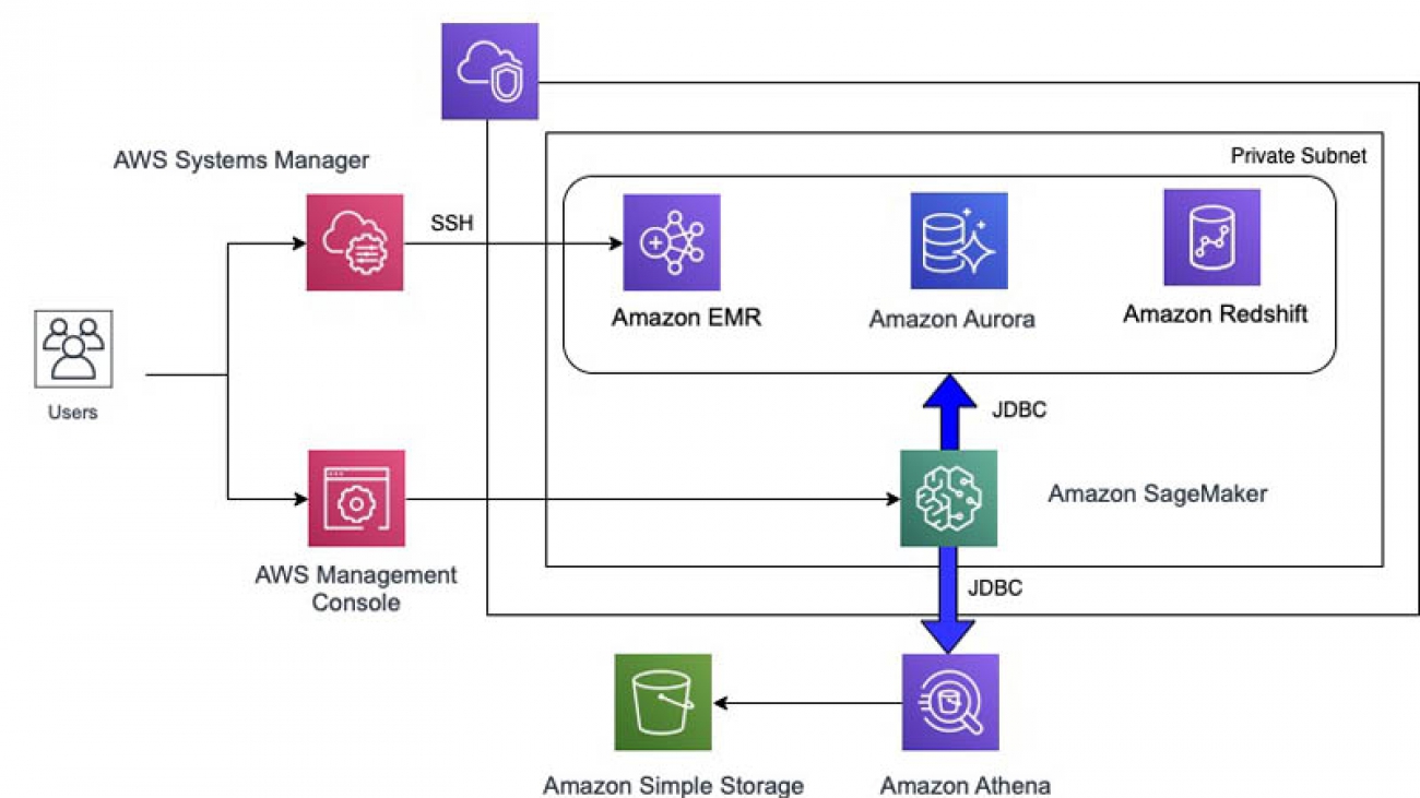
The following architecture diagram shows how you can use Amazon SageMaker to run code using the R kernel by establishing connectivity to various sources. You can also use the Amazon Redshift query editor or Amazon Athena query editor to create data resources. You need to use the Session Manager in AWS Systems Manager to SSH to the Amazon EMR cluster to create Hive resources.

Launching the AWS CloudFormation template

To automate resource creation, you run an AWS CloudFormation template. The template gives you the option to create an Amazon EMR cluster, Amazon Redshift cluster, or Amazon Aurora MySQL-compatible cluster automatically, as opposed to executing each step manually. It will take a few minutes to create all the resources.

  1. Choose the following link to launch the CloudFormation stack, which creates the required AWS resources to implement this solution:
  2. On the Create stack page, choose Next.
  3. Enter a stack name.
  4. You can change the default values for the following stack details:
Stack Details Default Values
Choose Second Octet for Class B VPC Address (10.xxx.0.0/16) 0
SageMaker Jupyter Notebook Instance Type ml.t2.medium
Create EMR Cluster Automatically? “Yes”
Create Redshift Cluster Automatically? “Yes”
Create Aurora MySQL DB Cluster Automatically? “Yes”
  1. Choose Next.
  2. On the Configure stack options page, choose Next.
  3. Select I acknowledge that AWS CloudFormation might create IAM resources.
  4. Choose Create stack.

You can now see the stack being created, as in the following screenshot.

When stack creation is complete, the status shows as CREATE_COMPLETE.

  1. On the Outputs tab, record the keys and their corresponding values.

You use the following keys later in this post:

  • AuroraClusterDBName – Aurora cluster database name
  • AuroraClusterEndpointWithPort – Aurora cluster endpoint address with port number
  • AuroraClusterSecret – Aurora cluster credentials secret ARN
  • EMRClusterDNSAddress – EMR cluster DNS name
  • EMRMasterInstanceId – EMR cluster primary instance ID
  • PrivateSubnets – Private subnets
  • PublicSubnets – Public subnets
  • RedshiftClusterDBName – Amazon Redshift cluster database name
  • RedshiftClusterEndpointWithPort – Amazon Redshift cluster endpoint address with port number
  • RedshiftClusterSecret – Amazon Redshift cluster credentials secret ARN
  • SageMakerNotebookName – Amazon SageMaker notebook instance name
  • SageMakerRS3BucketName – Amazon SageMaker S3 data bucket
  • VPCandCIDR – VPC ID and CIDR block

Creating your notebook with necessary R packages and JAR files

JDBC is an application programming interface (API) for the programming language Java, which defines how you can access a database. RJDBC is a package in R that allows you to connect to various data sources using the JDBC interface. The notebook instance that the CloudFormation template created ensures that the necessary JAR files for Hive, Presto, Amazon Athena, Amazon Redshift and MySQL are present in order to establish a JDBC connection.

  1. In the Amazon SageMaker Console, under Notebook, choose Notebook instances.
  2. Search for the notebook that matches the SageMakerNotebookName key you recorded earlier.
  3. Select the notebook instance.
  4. Click on “Open Jupyter” under “Actions” to locate the “jdbc” directory.

The CloudFormation template downloads the JAR files for Hive, Presto, Athena, Amazon Redshift, and Amazon Aurora MySQL-compatible inside the “jdbc” directory.

  1. Locate the lifecycle configuration attached.

A lifecycle configuration allows you to install packages or sample notebooks on your notebook instance, configure networking and security for it, or otherwise use a shell script for customization. A lifecycle configuration provides shell scripts that run when you create the notebook instance or when you start the notebook.

  1. Inside the Lifecycle configuration section, choose View script to see the lifecycle configuration script that sets up the R kernel in Amazon SageMaker to make JDBC connections to data sources using R.

It installs the RJDBC package and dependencies in the Anaconda environment of the Amazon SageMaker notebook.

Connecting to Hive and Presto

Amazon EMR is the industry-leading cloud big data platform for processing vast amounts of data using open source tools such as Apache Spark, Apache Hive, Apache HBase, Apache Flink, Apache Hudi, and Presto.

You can create a test table in Hive by logging in to the EMR master node from the AWS console using the Session Manager capability in Systems Manager. Systems Manager gives you visibility and control of your infrastructure on AWS. Systems Manager also provides a unified user interface so you can view operational data from multiple AWS services and allows you to automate operational tasks across your AWS resources. Session Manager is a fully managed Systems Manager capability that lets you manage your Amazon Elastic Compute Cloud (Amazon EC2) instances, on-premises instances, and virtual machines (VMs) through an interactive, one-click browser-based shell or through the AWS Command Line Interface (AWS CLI).

You use the following values from the AWS CloudFormation Outputs tab in this step:

  • EMRClusterDNSAddress – EMR cluster DNS name
  • EMRMasterInstanceId – EMR cluster primary instance ID
  • SageMakerNotebookName – Amazon SageMaker notebook instance name
  1. On the Systems Manager Console, under Instances & Nodes, choose Session Manager.
  2. Choose Start Session.
  3. Start an SSH session with the EMR primary node by locating the instance ID as specified by the value of the key EMRMasterInstanceId.

This starts the browser-based shell.

  1. Run the following SSH commands:
    # change user to hadoop 
    whoami
    sudo su - hadoop

  2. Create a test table in Hive from the EMR master node as you have already logged in using SSH:
    # Run on the EMR master node to create a table called students in Hive
    hive -e "CREATE TABLE students (name VARCHAR(64), age INT, gpa DECIMAL(3, 2));"
    
    # Run on the EMR master node to insert data to students created above
    hive -e "INSERT INTO TABLE students VALUES ('fred flintstone', 35, 1.28), ('barney rubble', 32, 2.32);"
    
    # Verify 
    hive -e "SELECT * from students;"
    exit
    exit

The following screenshot shows the view in the browser-based shell.

  1. Close the browser after exiting the shell.

To query the data from Amazon EMR using the Amazon SageMaker R kernel, you open the notebook the CloudFormation template created.

  1. On the Amazon SageMaker Console, under Notebook, chose Notebook instances.
  2. Find the notebook as specified by the value of the key SageMakerNotebookName.
  3. Choose Open Jupyter.
  4. To demonstrate connectivity from the Amazon SageMaker R kernel, choose Upload and upload the ipynb notebook.

    1. Alternatively, from the New drop-down menu, choose R to open a new notebook.
    2. Enter the code as mentioned in “hive_connect.ipynb”, replacing the emr_dns value with the value from key EMRClusterDNSAddress:
  5. Run all the cells in the notebook to connect to Hive on Amazon EMR using the Amazon SageMaker R console.

You follow similar steps to connect Presto:

  1. On the Amazon SageMaker Console, open the notebook you created.
  2. Choose Open Jupyter.
  3. Choose Upload to upload the ipynb notebook.
    1. Alternatively, from the New drop-down menu, choose R to open a new notebook.
    2. Enter the code as mentioned in “presto_connect.ipynb”, replacing the emr_dns value with the value from key EMRClusterDNSAddress:
  4. Run all the cells in the notebook to connect to PrestoDB on Amazon EMR using the Amazon SageMaker R console.

Connecting to Amazon Athena

Amazon Athena is an interactive query service that makes it easy to analyze data in Amazon Simple Storage Service (Amazon S3) using standard SQL. Amazon Athena is serverless, so there is no infrastructure to manage, and you pay only for the queries that you run. To connect to Amazon Athena from the Amazon SageMaker R kernel using RJDBC, we use the Amazon Athena JDBC driver, which is already downloaded to the notebook instance via the lifecycle configuration script.

You also need to set the query result location in Amazon S3. For more information, see Working with Query Results, Output Files, and Query History.

  1. On the Amazon Athena Console, choose Get Started.
  2. Choose Set up a query result location in Amazon S3.
  3. For Query result location, enter the Amazon S3 location as specified by the value of the key SageMakerRS3BucketName.
  4. Optionally, add a prefix, such as results.
  5. Choose Save.
  6. Create a database or schema and table in Athena with the example Amazon S3 data.
  7. Similar to connecting to Hive and Presto, to establish a connection from Athena to Amazon SageMaker using the R kernel, you can upload the ipynb notebook.
    1. Alternatively, open a new notebook and enter the code in “athena_connect.ipynb”, replacing the s3_bucket value with the value from key SageMakerRS3BucketName:
  8. Run all the cells in the notebook to connect to Amazon Athena from the Amazon SageMaker R console.

Connecting to Amazon Redshift

Amazon Redshift is a fast, fully managed cloud data warehouse that makes it simple and cost-effective to analyze all your data using standard SQL and your existing business intelligence (BI) tools. It allows you to run complex analytic queries against terabytes to petabytes of structured data, using sophisticated query optimization, columnar storage on high-performance storage, and massively parallel query execution. To connect to Amazon Redshift from the Amazon SageMaker R kernel using RJDBC, we use the Amazon Redshift JDBC driver, which is already downloaded to the notebook instance via the lifecycle configuration script.

You need the following keys and their values from the AWS CloudFormation Outputs tab:

  • RedshiftClusterDBName – Amazon Redshift cluster database name
  • RedshiftClusterEndpointWithPort – Amazon Redshift cluster endpoint address with port number
  • RedshiftClusterSecret – Amazon Redshift cluster credentials secret ARN

The CloudFormation template creates a secret for the Amazon Redshift cluster in AWS Secrets Manager, which is a service that helps you protect secrets needed to access your applications, services, and IT resources. Secrets Manager lets you easily rotate, manage, and retrieve database credentials, API keys, and other secrets throughout their lifecycle.

  1. On the AWS Secrets Manager Console, choose Secrets.
  2. Choose the secret denoted by the RedshiftClusterSecret key value.
  3. In the Secret value section, choose Retrieve secret value to get the user name and password for the Amazon Redshift cluster.
  4. On the Amazon Redshift Console, choose Editor (which is essentially the Amazon Redshift query editor).
  5. For Database name, enter redshiftdb.
  6. For Database password, enter your password.
  7. Choose Connect to database.
  8. Run the following SQL statements to create a table and insert a couple of records:
    CREATE TABLE public.students (name VARCHAR(64), age INT, gpa DECIMAL(3, 2));
    INSERT INTO public.students VALUES ('fred flintstone', 35, 1.28), ('barney rubble', 32, 2.32);
    

  9. On the Amazon SageMaker Console, open your notebook.
  10. Choose Open Jupyter.
  11. Upload the ipynb notebook.
    1. Alternatively, open a new notebook and enter the code as mentioned in “redshift_connect.ipynb”, replacing the values for RedshiftClusterEndpointWithPort, RedshiftClusterDBName, and RedshiftClusterSecret:
  12. Run all the cells in the notebook to connect to Amazon Redshift on the Amazon SageMaker R console.

Connecting to Amazon Aurora MySQL-compatible

Amazon Aurora is a MySQL-compatible relational database built for the cloud, which combines the performance and availability of traditional enterprise databases with the simplicity and cost-effectiveness of open-source databases. To connect to Amazon Aurora from the Amazon SageMaker R kernel using RJDBC, we use the MariaDB JDBC driver, which is already downloaded to the notebook instance via the lifecycle configuration script.

You need the following keys and their values from the AWS CloudFormation Outputs tab:

  • AuroraClusterDBName – Aurora cluster database name
  • AuroraClusterEndpointWithPort – Aurora cluster endpoint address with port number
  • AuroraClusterSecret – Aurora cluster credentials secret ARN

The CloudFormation template creates a secret for the Aurora cluster in Secrets Manager.

  1. On the AWS Secrets Manager Console, locate the secret as denoted by the AuroraClusterSecret key value.
  2. In the Secret value section, choose Retrieve secret value to get the user name and password for the Aurora cluster.

To connect to the cluster, you follow similar steps as with other services.

  1. On the Amazon SageMaker Console, open your notebook.
  2. Choose Open Jupyter.
  3. Upload the ipynb notebook.
    1. Alternatively, open a new notebook and enter the code as mentioned in “aurora_connect.ipynb”, replacing the values for AuroraClusterEndpointWithPort, AuroraClusterDBName, and AuroraClusterSecret:
  4. Run all the cells in the notebook to connect Amazon Aurora on the Amazon SageMaker R console.

Conclusion

In this post, we demonstrated how to connect to various data sources, such as Hive and PrestoDB on Amazon EMR, Amazon Athena, Amazon Redshift, and Amazon Aurora MySQL-compatible cluster, in your environment to analyze, profile, run statistical computions using R from Amazon SageMaker. You can extend this method to other data sources via JDBC.


Author Bio

Kunal Ghosh is a Solutions Architect at AWS. His passion is building efficient and effective solutions on the cloud, especially involving analytics, AI, data science, and machine learning. Besides family time, he likes reading, swimming, biking, and watching movies, and he is a foodie.


Gagan Brahmi is a Specialist Solutions Architect focused on Big Data & Analytics at Amazon Web Services. Gagan has over 15 years of experience in information technology. He helps customers architect and build highly scalable, performant, and secure cloud-based solutions on AWS.



Read More

Training a custom single class object detection model with Amazon Rekognition Custom Labels

Training a custom single class object detection model with Amazon Rekognition Custom Labels

Customers often need to identify single objects in images; for example, to identify their company’s logo, find a specific industrial or agricultural defect, or locate a specific event, like hurricanes, in satellite scans. In this post, we showcase how to train a custom model to detect a single object using Amazon Rekognition Custom Labels.

Amazon Rekognition is a fully managed service that provides computer vision (CV) capabilities for analyzing images and video at scale, using deep learning technology without requiring machine learning (ML) expertise. Amazon Rekognition Custom Labels lets you extend the detection and classification capabilities of the Amazon Rekognition pre-trained APIs by using data to train a custom CV model specific to your business needs. With the latest update to support single object training, Amazon Rekognition Custom Labels now lets you create a custom object detection model with single object classes.

Solution overview

To show you how the single class object detection feature works, we create a custom model to detect pizza in images. Because we only care about finding pizza in our images, we don’t want to create labels for other food types or create a “not pizza” label.

To create our custom model, we follow these steps:

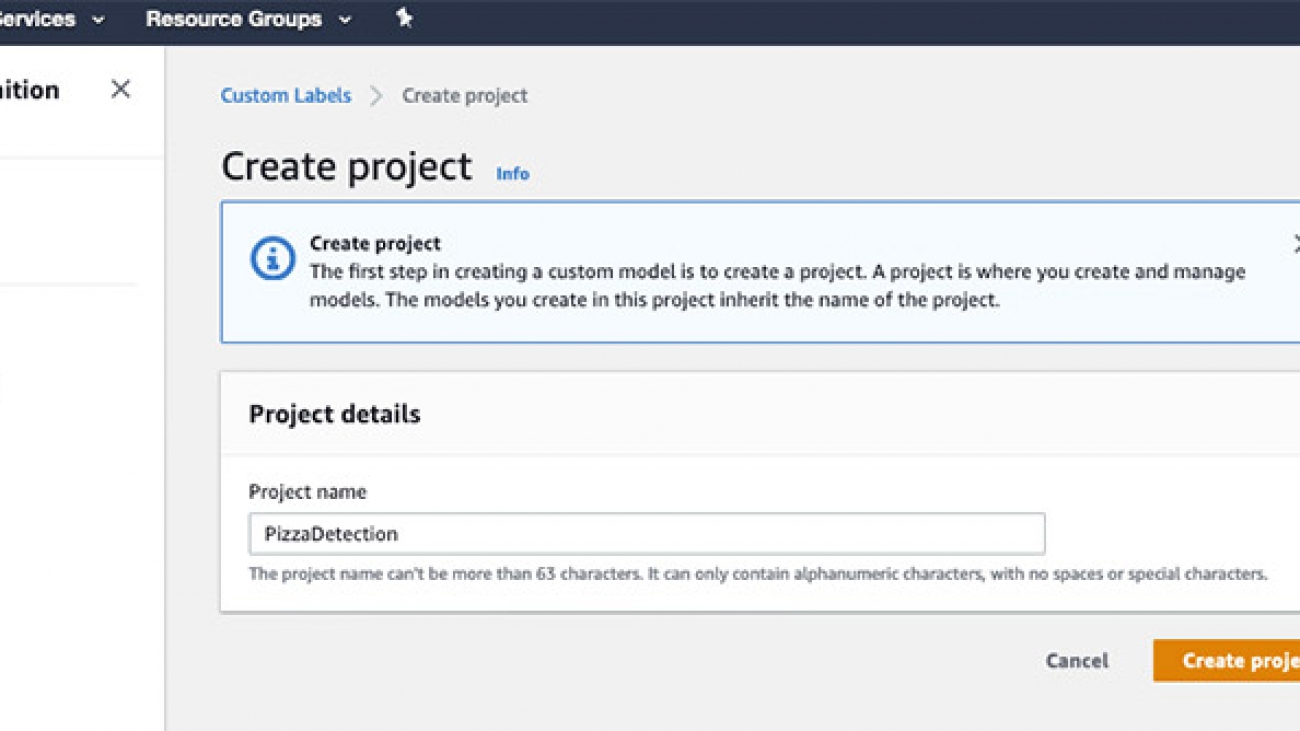
  1. Create a project in Amazon Rekognition Custom Labels.
  2. Create a dataset with images containing one or more pizzas.
  3. Label the images by applying bounding boxes on all pizzas in the images using the user interface provided by Amazon Rekognition Custom Labels.
  4. Train the model and evaluate the performance.
  5. Test the new custom model using the automatically generated API endpoint.

Amazon Rekognition Custom Labels lets you manage the ML model training process on the Amazon Rekognition console, which simplifies the end-to-end process.

Creating your project

To create your pizza-detection project, complete the following steps:

  1. On the Amazon Rekognition console, choose Custom Labels.
  2. Choose Get Started.
  3. For Project name, enter PizzaDetection.
  4. Choose Create project

You can also create a project on the Projects page. You can access the Projects page via the left navigation pane.

Creating your dataset

To create your pizza model, you first need to create a dataset to train the model with. For this post, our dataset is composed of 39 images that contain pizza. We sourced our images from pexels.com.

To create your dataset:

  1. Choose Create dataset.
  2. Select Upload images from your computer.

  1. Choose Add Images.
  2. Upload your images. You can always add more images later.

Labeling the images with bounding boxes

You’re now ready to label the images by applying bounding boxes on all images with pizza.

  1. Add Pizza as a label to your dataset via the labels list on the left side of the gallery.
  2. Apply the label to the pizzas in the images by selecting all the images with pizza and choosing Draw Bounding Box.

You can use the Shift key to automatically select multiple images between the first and last selected images.

Make sure to draw a bounding box that covers the pizza as tightly as possible.

Training your model

After you label your images, you’re ready to train your model.

  1. Choose Train Model.
  2. For Choose project, choose your PizzaDetection project.
  3. For Choose training dataset, choose your PizzaImages dataset.

As part of the training, Amazon Rekognition Custom Labels requires a labeled test dataset. You use the text dataset to verify how well the trained model predicts the correct labels and generate evaluation metrics. You don’t use the images in the test dataset to train your model; they should represent the types of images you want your model to analyze.

  1. For Create test set, choose how you want to provide your test dataset.

Amazon Rekognition Custom Labels provides three options:

  • Choose an existing test dataset
  • Create a new test dataset
  • Split training dataset

For this post, we select Split training dataset and let Amazon Rekognition hold back 20% of the images for testing and use the remaining 80% of the images to train the model.

Our model took approximately 1 hour to train. The training time required for your model depends on many factors, including the number of images provided in the dataset and the complexity of the model.

When training is complete, Amazon Rekognition Custom Labels outputs key metrics with every training, including F1 score, precision, recall, and the assumed threshold for each label. For more information about metrics, see Metrics for Evaluating Your Model.

Looking at our evaluation results, our model has a precision of 1.0, which means that no objects were mistakenly identified as pizza (false positives) in our test set. Our model did miss some pizzas in our test set (false negatives), which is reflected in our recall score of 0.81. You can often use the F1 score as an overall quality score because it takes both precision and recall into account. Finally, we see that our assumed threshold to generate the F1 score, precision, and recall metrics for Pizza is 0.61. By default, our model returns predictions above this assumed threshold. We can increase the recall for this model if we lower the confidence threshold. However, this would most likely cause a drop in precision.

We can also choose View Test Results to see each test image and how our model performed. The following screenshot shows an example of a correctly identified image of pizza during the model testing (true positive).

Testing your model

Your custom pizza detection model is now ready for use. Amazon Rekogntion Custom Labels provides the API calls for starting and using the model; you don’t need to deploy, provision, or manage any infrastructure. The following screenshot shows the API calls for using the model.

By using the API, we tried our model on a new test set of images from pexels.com.

For example, the following image shows a pizza on a table with other objects.

The model detects the pizza with a confidence of 91.72% and a correct bounding box. The following code is the JSON response received by the API call:

{
    "CustomLabels": [
        {
            "Name": "Pizza",
            "Confidence": 91.7249984741211,
            "Geometry": {
                "BoundingBox": {
                    "Width": 0.7824199795722961,
                    "Height": 0.3644999861717224,
                    "Left": 0.11868999898433685,
                    "Top": 0.37672001123428345
                }
            }
        }
    ]
}

The following image has a confidence score of 98.40.

The following image has a confidence score of 96.51.

The following image has an empty JSON result, as expected, because the image doesn’t contain pizza.

The following image also has an empty JSON result.

In addition to using the API, you can also use the Custom Labels Demonstration. This AWS CloudFormation template enables you to set up a custom, password-protected UI where you can start and stop your models and run demonstration inferences.

Conclusion

In this post, we showed you how to create a single class object detection model with Amazon Rekognition Custom Labels. This feature makes it easy to train a custom model that can detect an object class without needing to specify other objects or losing accuracy in its results.

For more information about using custom labels, see What Is Amazon Rekognition Custom Labels?


About the Author

Woody Borraccino is a Senior AI Solutions Architect at AWS.


Read More

A Simulation Suite for Tackling Applied Reinforcement Learning Challenges

A Simulation Suite for Tackling Applied Reinforcement Learning Challenges

Posted by Daniel J. Mankowitz, Research Scientist, DeepMind and Gabriel Dulac-Arnold, Research Scientist, Google Research

Reinforcement Learning (RL) has proven to be effective in solving numerous complex problems ranging from Go, StarCraft and Minecraft to robot locomotion and chip design. In each of these cases, a simulator is available or the real environment is quick and inexpensive to access. Yet, there are still considerable challenges to deploying RL to real-world products and systems. For example, in physical control systems, such as robotics and autonomous driving, RL controllers are trained to solve tasks like grasping objects or driving on a highway. These controllers are susceptible to effects such as sensor noise, system delays, or normal wear-and-tear that can reduce the quality of input to the controller, leading to incorrect decision-making and potentially catastrophic failures.

A physical control system: Robots learning how to grasp and sort objects using RL at the Everyday Robot Project at X. These types of systems are subject to many of the real-world challenges detailed here.

In “Challenges of Real-World Reinforcement Learning”, we identify and discuss nine different challenges that hinder the application of current RL algorithms to applied systems. We then follow up this work with an empirical investigation in which we simulated versions of these challenges on state-of-the-art RL algorithms, and benchmark the effects of each. We have open-sourced these simulated challenges in the Real-World RL (RWRL) task suite to help draw attention to these important issues, as well as accelerate research toward solving them.

The RWRL Suite
The RWRL suite is a set of simulated tasks inspired by applied reinforcement learning challenges, the goal of which is to enable fast algorithmic iterations for both researchers and practitioners, without having to run slow, expensive experiments on real-systems. While there will be additional challenges transitioning from RL algorithms that were trained in simulation to real-world applications, this suite intends to close some of the more fundamental, algorithmic gaps. At present, RWRL supports a subset of the DeepMind Control Suite domains, but the goal is to broaden the suite to support an even more diverse domain set.

Easy-to-Use & Flexible
We designed the suite with two main goals in mind. (1) It should be easy to use — a user should be able to start running experiments within minutes of downloading the suite, simply by changing a few lines of code. (2) It should be flexible — a user should be able to incorporate any combination of challenges into the environment with very little effort.

A Delayed Action Example
To illustrate the ease of use of the RWRL suite, imagine a researcher or practitioner wants to implement action delays (i.e., temporal delays on actions being sent to the environment). To use the RWRL suite, simply import the rwrl module. Next, load an environment (e.g., cartpole) with the delay_spec argument. This optional argument is specified as a dictionary configuring delay applied to actions, observations, or rewards and the number of timesteps the corresponding element is delayed (e.g., 20 timesteps). Once the environment is loaded, the effects of actions are automatically delayed without any other changes to the experiment. This makes it easy to test an RL algorithm with action delays in a range of different environments supported by the RWRL suite.

A high-level overview of the RWRL suite. Add a challenge (e.g., action delays) into the environment with a few lines of code, run a hyperparameter sweep and produce a graph shown on the right

A user can combine different challenges or choose from a set of predefined benchmark challenges by simply adding additional arguments to the load function, all of which are specified in the open-source RWRL suite codebase.

Supported Challenges
The RWRL suite provides functionality to support experiments related to eight of the nine different challenges that make applying current RL algorithms on applied systems difficult: sample efficiency; system delays; high-dimensional state and action spaces; constraints; partial observability, stochasticity and non-stationarity; multiple objectives; real-time inference; and training from offline logs. RWRL excludes the explainability challenge, which is abstract and non-trivial to define. The supported experiments are non-exhaustive and provide researchers and practitioners with the ability to analyze the capabilities of their agent with respect to each challenge dimension. Examples of the supported challenges include:

  • System Delays
    Most real systems have delays in either sensing, actuation or reward feedback, all of which can be configured and applied to any task within the RWRL suite.The graphs below show the performance of a D4PG agent as actions (left), observations (middle) and rewards (right) are increasingly delayed.
    The effect of increasing the action (left), observation (middle) and reward (right) delays respectively on a state-of-the art RL agent in four MuJoCo domains.

    As can be seen in the graphs, a researcher or practitioner can quickly gain insights as to which type of delay affects their agent’s performance. These delays can also be combined together to observe their combined effect.

  • Constraints
    Almost all applied systems have some form of constraints embedded into the overall objective, which is not common in most RL environments. The RWRL suite implements a series of constraints for each task, with varying difficulties, to facilitate research in constrained RL. An example of a complex local angular velocity constraint being violated is visualized in the video below.
    An example of constraint violations for cartpole. The red screen indicates that a violation has occurred on localized angular velocity.
  • Non-Stationarity
    The user can introduce non-stationarity by perturbing environment parameters. These perturbations are in contrast to the pixel level adversarial perturbations that have recently gained popularity in research on supervised deep learning. For example, in the human walker domain, the size of the head and friction of the ground can be modified throughout training to simulate changing conditions. A variety of schedulers are available in the RWRL suite (see our codebase for more details), along with multiple default parameter perturbations, which were carefully defined to handicap the learning capabilities of state-of-the-art learning algorithms.
    Non-stationary perturbations. The suite supports perturbing environment parameters across episodes such as changing head size (center) and contact friction (right).
  • Training from Offline Log Data
    In most applied systems, it is both slow and expensive to run experiments. There are often logs of data available from previous experiments that can be utilized to train a policy. However, it is often difficult to outperform the previous model in production due to the data being limited, of low variance, or of poor quality. To address this, we have generated offline datasets of the combined RWRL benchmark challenges, which we made available as part of a wider offline dataset release. More information can be found in this notebook.

Conclusion
Most systems rarely manifest only a single challenge, and we are excited to see how algorithms can deal with an environment in which there are multiple challenges combined with increasing levels of difficulty (‘Easy’, ‘Medium’ and ‘Hard’). We highly encourage the research community to try and solve these challenges, as we believe that solving them will facilitate more widespread applications of RL to products and real-world systems.

While the initial set of RWRL suite features and experiments provide a starting point for closing the gap between the current state of RL and the challenges of applied systems, there is still much work to do. The supported experiments are not exhaustive and we welcome new ideas from the wider community to better evaluate the capabilities of our RL agents. Our main goal with this suite is to highlight and encourage research on the core problems that limit the effectiveness of RL algorithms in applied products and systems and to accelerate progress towards enabling future RL applications.

Acknowledgements
We would like to thank our core contributor and co-author Nir Levine for his invaluable help. We would also like to thank our co-authors Jerry Li, Sven Gowal, Todd Hester and Cosmin Paduraru as well as Robert Dadashi, the ACME team, Dan A. Calian, Juliet Rothenberg and Timothy Mann for their contributions.

Read More

Population mobility, small business closures, and layoffs during the COVID-19 pandemic

Population mobility, small business closures, and layoffs during the COVID-19 pandemic

Global findings from the Future of Business Survey and Facebook Movement Range Maps

Since the onset of the COVID-19 pandemic, Facebook’s Data for Good Program has been sharing insights with nonprofits, researchers, and public health officials to support the global response. Data for Good shares aggregate statistics on things like whether people are generally staying put in response to stay-at-home policies, as well as perspectives shared from our online community of 150 million businesses about how the pandemic has affected their operations. Using data from several Facebook data sets, we examine the extent to which population mobility influences business outcomes. We find that declines in country-level mobility are heavily correlated with a higher share of small and medium businesses (SMBs) on Facebook reporting layoffs, as well as with the proportion of small businesses having completely closed due to the pandemic.

Data sources

Future of Business Survey

The Future of Business Survey is an ongoing collaboration between Facebook Data for Good, the Organisation for Economic Co-operation and Development (OECD), and the World Bank to survey online small and medium businesses on the Facebook platform about their conditions, challenges, and operations. To provide timely information in response to the COVID-19 outbreak, the Future of Business has shifted to a monthly sampling frame that aims to assess SMBs’ responses to the pandemic in more than 50 countries.

In May, the Future of Business surveyed over 30,000 small businesses around the world and found that, during the pandemic, more than one in four had closed and one in three had laid off workers. In June, we conducted a follow-up survey among 25,000 small business owners and managers and found that as many countries had begun to ease their lockdown restrictions, some businesses were able to resume their in-person operations but nearly one in five (18 percent) businesses remained closed.

Movement Range Maps

Part of Facebook’s Disease Prevention Maps toolkit, Movement Range Maps are intended to inform researchers and public health experts about how populations are responding to physical distancing measures. To analyze how population mobility shifts as stay-at-home orders are put into place, these maps calculate a “change in movement” metric, which looks at how much people are moving around and compares it with a baseline period that predates social distancing measures. This data is derived from people who are using Facebook on a mobile device and who have opted in to the Location History feature. When publishing Movement Range Maps, we aggregate observations to a county level and add random noise to protect privacy.

Analysis

Effects on employment

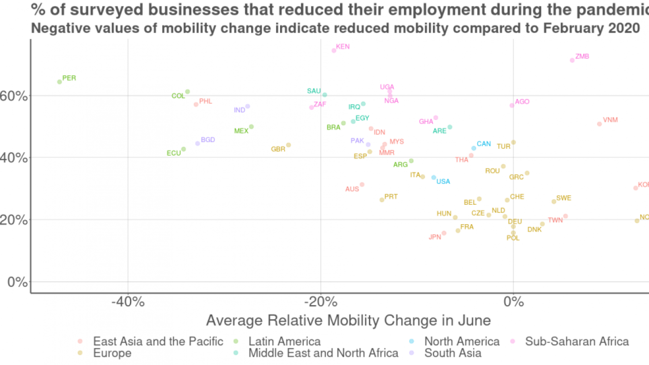
To compute a weighted average of relative change of mobility for each country, we took the publicly available movement range data by region and divided it by the number of observations in each subnational unit in the country. We then analyzed the correlation between relative changes in mobility and small business layoffs at the country level as reported in the Future of Business for the month of June, examining businesses that reported having been fully closed as well as businesses that remained open. We see that the percent of businesses that laid off employees is correlated with drops in mobility (coefficient = –0.54) and that a higher proportion of small businesses in sub-Saharan Africa and Latin America laid off workers as compared with those in the European region.

To check for robustness, we also fit a simple linear regression, including the region of the country as a fixed effect to see whether the relationship between mobility rates and layoffs remained after controlling for geographic influences. When we control for region, the estimated coefficient of relative mobility remains negative (–0.42) and statistically significant (p < 0.01), suggesting that country-level declines in mobility have a unique and significant effect on small business layoffs even when controlling for a broader set of regional factors.

We then analyzed the correlation between relative changes in mobility during the month of June and small businesses closures. This analysis revealed that countries with the lowest levels of mobility had more businesses closed during the pandemic and countries with higher overall mobility had the fewer closures (coefficient = –0.73).

When we include regional fixed effects, the estimated coefficient of the mobility change was –0.41 and statistically significant (p < 0.001), suggesting that every percentage point drop in mobility in June was associated with a 0.41 percentage point increase in the business closure rates during the pandemic, independent of regional influences.

Conclusion

Analyzing June data from the Future of Business Survey and Movement Range Maps, we find that declines in mobility are strongly correlated with layoffs as well as business closure rates at a country level. These findings suggest that as states, cities, and countries face COVID-19 outbreaks and corresponding lockdowns, small businesses will continue to experience closures and layoffs. As a result, the small business community is likely to continue to need support over the coming year from local and international institutions that are seeking to help business owners mitigate the effects of the pandemic.

Data from this research blog, including the Future of Business Survey and Movement Range Maps, is shared publicly in an effort to better help respond to the COVID-19 pandemic. To access Facebook’s publicly available data sets, please visit our page on Humanitarian Data Exchange.

The post Population mobility, small business closures, and layoffs during the COVID-19 pandemic appeared first on Facebook Research.

Read More

Here Comes the Sun: NASA Scientists Talk Solar Physics

Here Comes the Sun: NASA Scientists Talk Solar Physics

Michael Kirk and Raphael Attie, scientists at NASA’s Goddard Space Flight Center, regularly face terabytes of data in their quest to analyze images of the sun.

This computational challenge, which could take a year or more on a CPU, has been reduced to less than a week on Quadro RTX data science workstations. Kirk and Attie spoke to AI Podcast host Noah Kravitz about the workflow they follow to study these images, and what they hope to find.

The lessons they’ve learned are useful for those in both science and industry grappling with how to best put torrents of data to work.

The researchers study images captured by telescopes on satellites, such as the Solar Dynamics Observatory spacecraft, as well as those from ground-based observatories.

They study these images to identify particles in Earth’s orbit that could damage interplanetary spacecraft, and to track solar surface flows, which allow them to develop models predicting weather in space.

Currently, these images are taken in space and sent to Earth for computation. But Kirk and Attie aim to shoot for the stars in the future: the goal is the ultimate form of edge computing, putting high-performance computers in space.

Key Points From This Episode:

  • The primary instrument that Kirk and Attie use to see images of the sun is the Solar Dynamics Observatory, a spacecraft that has four telescopes to take images of the extreme ultraviolet light of the sun, as well as an additional instrument to measure its magnetic fields.
  • Researchers such as Kirk and Attie have developed machine learning algorithms for a variety of projects, such as creating synthetic images of the sun’s surface and its flow fields.

Tweetables:

“We take an image about once every 1.3 seconds of the sun … that entire data archive — we’re sitting at about 18 petabytes right now.” — Michael Kirk [6:50]

“What AI is really offering us is a way to crunch through terabytes of data that are very difficult to move back to Earth.” — Raphael Attie [34:34]

You Might Also Like

How the Breakthrough Listen Harnessed AI in the Search for Aliens

UC Berkeley’s Gerry Zhang talks about his work using deep learning to analyze signals from space for signs of intelligent extraterrestrial civilizations. And while we haven’t found aliens yet, the doctoral student has already made some extraordinary discoveries.

Forget Storming Area 51, AI’s Helping Astronomers Scour the Skies for Habitable Planets

Astronomer Olivier Guyon and professor Damien Gratadour speak about the quest to discover nearby habitable planets using GPU-powered extreme adaptive optics in very large telescopes.

Astronomers Turn to AI as New Telescopes Come Online 

To turn the vast quantities of data that will be pouring out of new telescopes into world-changing scientific discoveries, Brant Robertson, a visiting professor at the Institute for Advanced Study in Princeton and an associate professor of astronomy at UC Santa Cruz, is turning to AI.

The post Here Comes the Sun: NASA Scientists Talk Solar Physics appeared first on The Official NVIDIA Blog.

Read More

Increasing the relevance of your Amazon Personalize recommendations by leveraging contextual information

Increasing the relevance of your Amazon Personalize recommendations by leveraging contextual information

Getting relevant recommendations in front of your users at the right time is a crucial step for the success of your personalization strategy. However, your customer’s decision-making process shifts depending on the context at the time when they’re interacting with your recommendations. In this post, I show you how to set up and query a context-aware Amazon Personalize deployment.

Amazon Personalize allows you to easily add sophisticated personalization capabilities to your applications by using the same machine learning (ML) technology used on Amazon.com for over 20 years. No ML experience is required. Amazon Personalize supports the automatic adjustment of recommendations based on contextual information about your user, such as device type, location, time of day, or other information you provide.

The Harvard study How Context Affects Choice defines context as factors that can influence the choice outcome by altering the process by which a decision is made. As a business owner, you can identify this context by analyzing how your customers shop differently when accessing your catalog from a phone vs. a computer, or seeing the shift in your customer’s content consumption on rainy vs. sunny days.

Leveraging your user’s context allows you to provide a more personalized experience for existing users and helps decrease the cold-start phase for new or unidentified users. The cold-start phase refers to the period when your recommendation engine provides non-personalized recommendations due to the lack of historical information regarding that user.

Adding context to Amazon Personalize

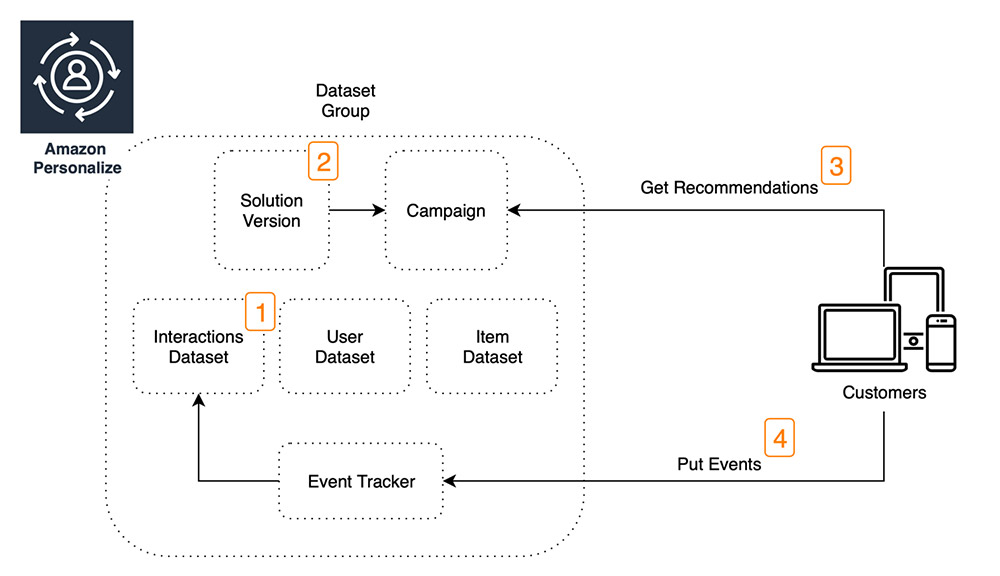
You can set up and use context in Amazon Personalize in four simple steps:

  1. Include your user’s context in the historical user-item interactions dataset.
  2. Train a context aware solution with a User Personalization or Personalized Ranking recipe. A recipe refers to the algorithm your recommender is trained on using the behavioral data specified in your interactions dataset plus any user or items metadata.
  3. Specify the user’s context when querying for real-time recommendations using the GetRecommendations or GetPersonalizedRanking
  4. Include your user’s context when recording events using the event tracker.

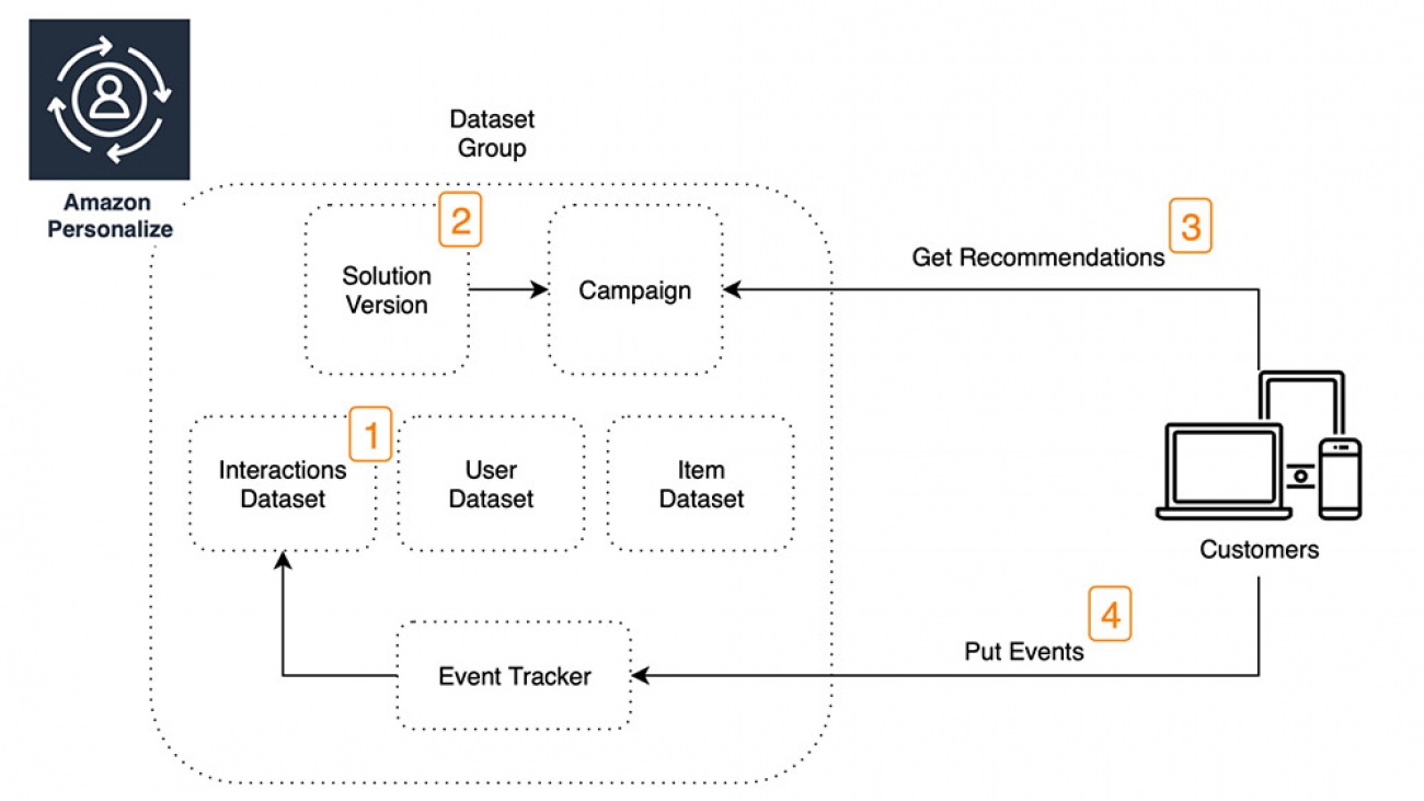
The following diagram illustrates the architecture of these steps.

You want to be explicit about the context to consider when constructing datasets. A common example of context customers actively use is device type, such as a phone, tablet, or desktop. The study The Effect of Device Type on Buying Behavior in Ecommerce: An Exploratory Study from the University of Twente in the Netherlands has proven that device type has an influence on buying behavior and people might postpone a buying decision if they’re online with the wrong device type. Embedding device type context in your datasets allows Amazon Personalize to learn this pattern and, at inference time, recommend the most appropriate content with awareness of the user’s context.

Recommendations use case

For this use case, a travel enthusiast is our potential customer. They look at a few things when deciding which airline to travel with to their given destination. For example, is it a short or a long flight? Will the trip be booked with cash or with miles? Are they traveling alone? Where are they be departing and returning to? After they answer these initial questions, the next big decision is picking the cabin type to fly in. If our travel enthusiast is flying in a high-end cabin type, we can assume they’re looking at which airline provides the best experience possible. Now that we have a good idea on what our user is looking for, it’s shopping time!

Consider some of the variables that go into the decision-making process of this use case. We can’t control many of these factors, but we can use some to tailor our recommendations. First, identify common denominators that might affect a user’s behavior. In this case, flight duration and cabin type are good candidates to use as context, and traveler type and traveler residence are good candidates for user metadata when building our recommendation datasets. Metadata is information you know about your users and items that stays somewhat constant over a period of time, whereas context is environmental information that can shift rapidly across time, influencing your customer’s perception and behavior.

Selecting the most relevant metadata fields in your training datasets and enriching your interactions datasets with context is important for generating relevant user recommendations. In this post, we build an Amazon Personalize deployment that returns a list of airline recommendations for a customer. We add cabin type as the context and traveler residence as the metadata field and observe how recommendations shift based on context and metadata.

Prerequisites

We first need to set up the following Amazon Personalize resources. For full instructions, see Getting Started (Console) to complete the following steps:

  1. Create a dataset group. In this post, we name it airlines-blog-example.
  2. Create an Interactions dataset using the following schema and import data using the interactions_dataset.csv file:
    {
      "type": "record",
      "name": "Interactions",
      "namespace": "com.amazonaws.personalize.schema",
      "fields": [
    {
              "name": "ITEM_ID",
              "type": "string"
          },
          {
              "name": "USER_ID",
              "type": "string"
          },
          {
              "name": "TIMESTAMP",
              "type": "long"
          },
          {
              "name":"CABIN_TYPE",
              "type": "string",
              "categorical": true
          },
          {
            "name": "EVENT_TYPE",
            "type": "string"
          },
          {
            "name": "EVENT_VALUE",
            "type": "float"
          }
      ],
      "version": "1.0"
    }

  3. Create a Users dataset using the following schema and import data using the users_dataset.csv file:
    {
      "type": "record",
      "name": "Users",
      "namespace": "com.amazonaws.personalize.schema",
      "fields": [
        {
          "name": "USER_ID",
          "type": "string"
        },
        {
          "name": "USER_RESIDENCE",
          "type": "string",
          "categorical": true
        }
      ],
      "version": "1.0"
    }

  4. Create a solution. In this post, we use the default solution configurations, except for the following:
    1. Recipeaws-hrnn-metadata
    2. Event type – RATING
    3. Perform HPO – True

Hyperparameter optimization (HPO) is recommended if you want Amazon Personalize to run parallel trainings and experiments to identify the most performant hyperparameters. For more information, see Hyperparameters and HPO.

  1. Create a campaign.

You can set up the preceding resources on the Amazon Personalize console or by following the Jupyter notebook personalize_hrnn_metadata_contextual_example.ipynb example on the GitHub repo.

Exploring your Amazon Personalize resources

We have now created several Amazon Personalize resources, including a dataset group called airlines-blog-example. The dataset group contains two datasets: interactions and users, which contain the data used to train your Amazon Personalize model (also known as a solution). We also created a campaign to provide real-time recommendations.

We can now explore how the interactions and users dataset schemas help our model learn from the context and metadata embedded in the datasets.

Interactions dataset

We provide Amazon Personalize an interactions dataset with a numeric rating (combination of EVENT_TYPE + EVENT_VALUE) that a user (USER_ID) has given an airline (ITEM_ID) when flying in a certain cabin type (CABIN_TYPE) at a given time (TIMESTAMP). By providing this information to Amazon Personalize in the dataset and schema, we can add CABIN_TYPE as the context when querying the recommendations for a user and recording new interactions through the event tracker. At training time, the model automatically identifies important features from this data (for our use case, the highest rated airlines across cabin types).

The following screenshot showcases a small portion of the interactions_dataset.csv file.

User dataset

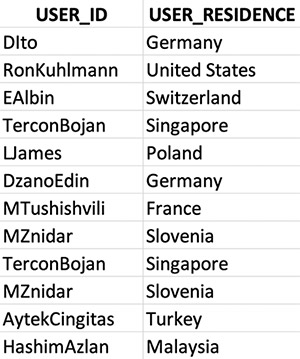
We also provide Amazon Personalize a user dataset with the users (USER_ID) who provided the ratings in the interactions dataset, assuming that they gave the rating from their country of residence (USER_RESIDENCE). In this use case, USER_RESIDENCE is the metadata we picked for these users. By providing USER_RESIDENCE as user metadata, the model can learn which airlines are interacted with the most by users across countries and regions, so when we query for recommendations, it takes USER_RESIDENCE in consideration. For example, users in Asia see different airline options compared to users in South America or Europe.

The following screenshot shows a small portion of the user_dataset.csv file.

The raw dataset of user airlines ratings from Skytrax contains 20 columns with over 40,000 records. In this post, we use a modified version of this dataset and split the most relevant columns of the raw dataset into two datasets (users and interactions). For more information about splitting the data in a Jupyter notebook, see personalize_hrnn_metadata_contextual_example.ipynb on the GitHub repo.

The next section shows how context and metadata influence the real-time recommendations provided by your Amazon Personalize campaign.

Applying context to your Amazon Personalize real-time recommendations queries

During this test, we observe the effect that context has on the recommendations provided to users. In our use case, we have an interactions dataset of numerical airline ratings from multiple users. In our schemas, the cabin type is included as a categorical value for the interactions dataset and the user residence as a metadata field in the users dataset. Our theory is that by adding the cabin type as context, the airline recommendations will shift to account for it.

  1. On your Amazon Personalize dataset group dashboard, choose View campaigns.
  2. Choose your newly created campaign.
  3. For User ID, enter JDowns.
  4. Choose Get recommendations.

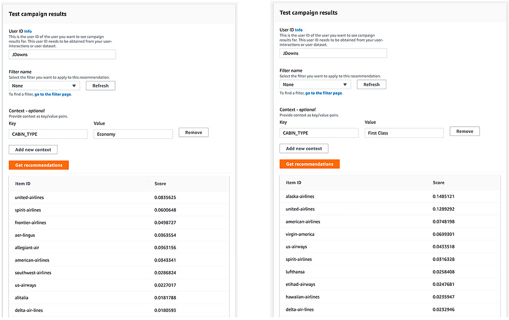
You should see a Test campaign results page similar to the following screenshot.

We initially queried a list of airlines for our user without any context. We now focus on the top 10 recommendations and verify that they shift based on the context. We can add the context via the console by providing a key and value pair. In our use case, the key is CABIN_TYPE and the value can be one of the following:

  • Economy
  • Premium Economy
  • Business Class
  • First Class

The following two screenshots show our results for querying recommendations for the same user with Economy and First Class as values for the CABIN_TYPE context. The economy context doesn’t shift the top 10 list, but the first class context does have an effect—bumping Alaska Airlines to first place on the list.

You can explore your users_dataset.csv file for additional users to test your recommendations API, and a very similar shift of recommendations based on the context you include in the API call. You can also find that the airlines list shifts based on the User Residency metadata field. For example, the following screenshots show the top 10 recommendations for our JDowns user, who has United States as the value for User Residency, compared to the PhillipHarris user, who has France as the value for User Residency.

Conclusion

As shown in this post, adding context to your recommendation strategy is a very powerful and easy-to-implement exercise when using Amazon Personalize. The benefits of enriching your recommendations with context can result in an increase in your user engagement, which eventually leads to an increase in the revenue influenced by your recommendations.

This post showed you how to create an Amazon Personalize context-aware deployment and an end-to-end test of getting real-time recommendations applying context via the Amazon Personalize console. For instructions on using a Jupyter environment to set up the Amazon Personalize infrastructure and get recommendations using the Boto3 Python SDK, see personalize_hrnn_metadata_contextual_example.ipynb on the GitHub repo.

There’s even more that you can do with Amazon Personalize. For more information about core use cases and automation examples, see the GitHub repo.

If this post helps you or inspires you to solve a problem, share your thoughts and questions in the comments.


About the Author

Luis Lopez Soria is an AI/ML specialist solutions architect working with the AWS machine learning team. He works with AWS customers to help them adopt machine learning on a large scale. He enjoys playing sports, traveling around the world, and exploring new foods and cultures.


Read More

Amazon Forecast can now use Convolutional Neural Networks (CNNs) to train forecasting models up to 2X faster with up to 30% higher accuracy

Amazon Forecast can now use Convolutional Neural Networks (CNNs) to train forecasting models up to 2X faster with up to 30% higher accuracy

We’re excited to announce that Amazon Forecast can now use Convolutional Neural Networks (CNNs) to train forecasting models up to 2X faster with up to 30% higher accuracy. CNN algorithms are a class of neural network-based machine learning (ML) algorithms that play a vital role in Amazon.com’s demand forecasting system and enable Amazon.com to predict demand for over 400 million products every day. For more information about Amazon.com’s journey building demand forecasting technology using CNN models, watch the re:MARS 2019 keynote video. Forecast brings the same technology used at Amazon.com into the hands of everyday developers as a fully managed service. Anyone can start using Forecast, without any prior ML experience, by using the Forecast console or the API.

Forecasting is the science of predicting the future. By examining historical trends, businesses can make a call on what might happen and when, and build that into their future plans for everything from product demand to inventory to staffing. Given the consequences of forecasting, accuracy matters. If a forecast is too high, businesses over-invest in products and staff, which ends up as wasted investment. If the forecast is too low, they under-invest, which leads to a shortfall in inventory and a poor customer experience. Today, businesses try to use everything from simple spreadsheets to complex financial planning software to generate forecasts, but high accuracy remains elusive for two reasons:

  • Traditional forecasts struggle to incorporate very large volumes of historical data, missing out on important signals from the past that are lost in the noise.
  • Traditional forecasts rarely incorporate related but independent data, which can offer important context (such as sales, holidays, locations, and marketing promotions). Without the full history and the broader context, most forecasts fail to predict the future accurately.

At Amazon, we have learned over the years that no one algorithm delivers the most accurate forecast for all types of data. Traditional statistical models have been useful in predicting demand for products that have regular demand patterns, such as sunscreen lotions in the summer and woolen clothes in the winter. However, statistical models can’t deliver accurate forecasts for more complex scenarios, such as frequent price changes, differences between regional versus national demand, products with different selling velocities, and the addition of new products. Sophisticated deep learning models can provide higher accuracy in these use cases. Forecast automatically examines your data and selects the best algorithm across a set of statistical and deep learning algorithms to train the more accurate forecasting model for your data. With the addition of the CNN-based deep learning algorithm, Forecast can now further improve accuracy by up to 30% and train models up to 2X faster compared to the currently supported algorithms. This new algorithm can more accurately detect leading indicators of demand, such as pre-order information, product page visits, price changes, and promotional spikes, to build more accurate forecasts.

More Retail, a market leader in the fresh food and grocery category in India, participated in a beta test of the new CNN algorithm, with the help of Ganit, an analytics partner. Supratim Banerjee, Chief Transformation Officer at More Retail Limited, says, “At More, we rapidly innovate to sustain our business and beat competition. We have been looking for opportunities to reduce wastage due to over stocking, while continuing to meet customer demand. In our experiments for the fresh produce category, we found the new CNN algorithm in Amazon Forecast to be 1.7X more accurate compared to our existing forecasting system. This translates into massive cost savings for our business.”

Training a CNN predictor and creating forecasts

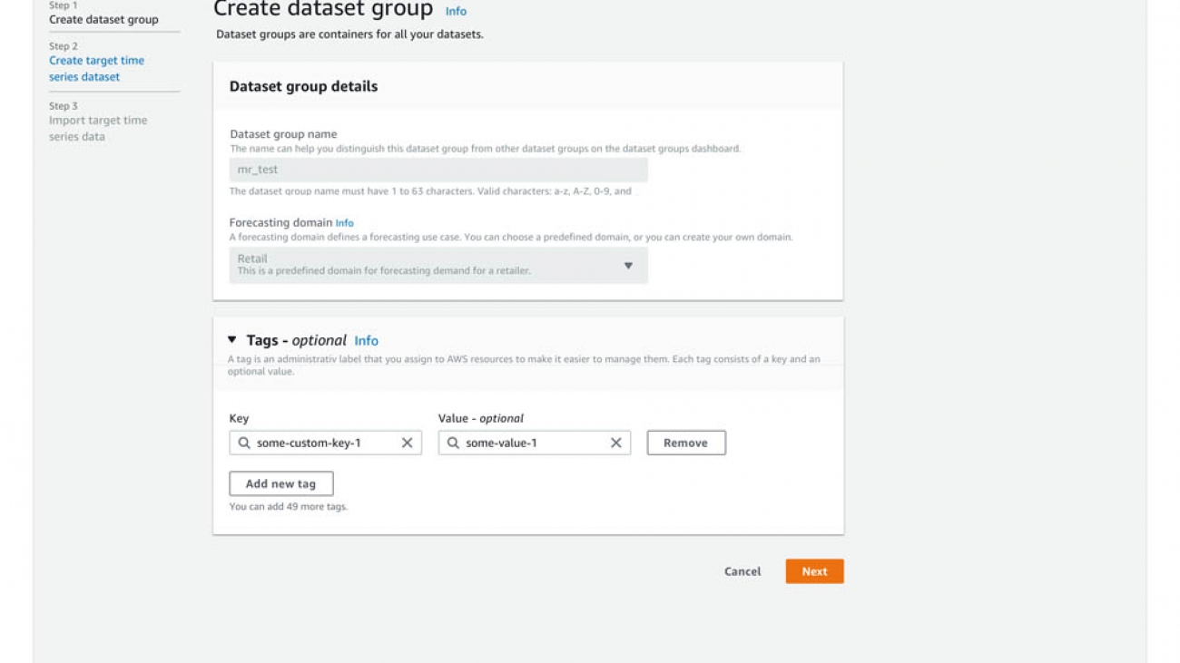
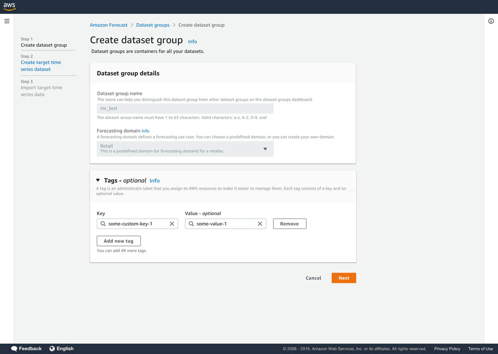
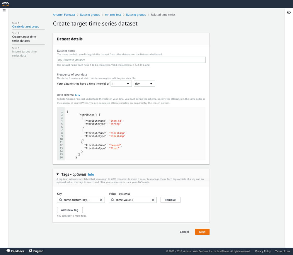
You can start using CNNs in Forecast through the CreatePredictor API or on the Forecast console. In this section, we walk through a series of steps required to train a CNN predictor and create forecasts within Forecast.

  1. On the Forecast console, create a dataset group.

  1. Upload your dataset.

  1. Choose Predictors from the navigation pane.
  2. Choose Train predictor.

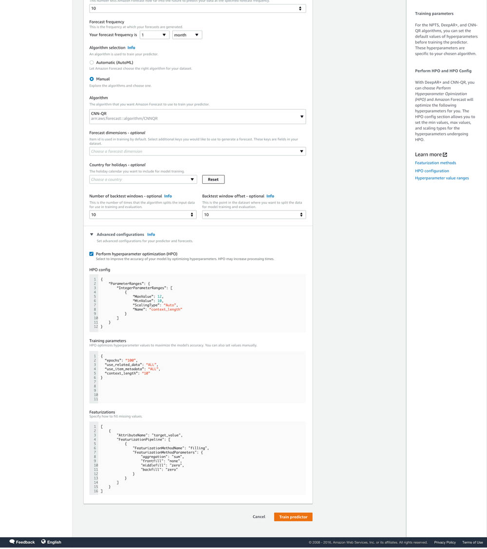
  1. For Algorithm selection, select Manual.
  2. For Algorithm, choose CNN-QR.

To manually select CNN-QR through the CreatePredictor API, use arn:aws:forecast:::algorithm/CNN-QR for the AlgorithmArn.

When you choose CNN-QR from the drop-down menu, the Advanced Configuration section auto-expands.

  1. To let Forecast train the most optimized and accurate CNN model for your data, select Perform hyperparameter optimization (HPO).
  2. After you enter all your details on the Predictors page, choose Train predictor.

After your predictor is trained, you can view its details by choosing your predictor on the Predictors page. On the predictor’s details page, you can view the accuracy metrics and optimized hyperparameters for your model.

  1. Now that your model is trained, choose Forecasts from the navigation name.
  2. Choose Create a forecast.
  3. Create a forecast using your trained predictor.

You can generate forecasts at any quantile to balance your under-forecasting and over-forecasting costs.

Choosing the most accurate model with Forecast

With this launch, Forecast now supports one proprietary CNN model, one proprietary RNN model, and four other statistical models: Prophet, NPTS (Amazon proprietary), ARIMA, and ETS. The new CNN model is part of AutoML. We recommend always starting your experimentation with AutoML, in which Forecast finds the most optimized and accurate model for your dataset.

  1. On the Train predictor page, for Algorithm selection, select Automatic (AutoML).

  1. After your predictor is trained using AutoML, choose the predictor to see more details on the chosen algorithm.
  2. On the predictor’s details page, in the Algorithm metrics section, choose different algorithms from the drop-down menu to view their accuracy for comparison.

Tips and best practices

As you begin to experiment with CNNs and build your demand planning solutions on top of Forecast, consider the following tips and best practices:

  • For experimentation, start by identifying the most important item IDs for your business that you are looking to improve your forecasting accuracy. Measure the accuracy of your existing forecasting methodology as a baseline.
  • Use Forecast with only your target time series and assess the wQuantileLoss accuracy metric. We recommend selecting AutoML in Forecast to find the most optimized and accurate model for your data. For more information, see Evaluating Predictor Accuracy.
  • AutoML optimizes for accuracy and not training time, so AutoML may take longer to optimize your model. If training time is a concern for you, we recommend manually selecting CNN-QR and assessing its accuracy and training time. A slight degradation in accuracy may be an acceptable trade-off for considerable gains in training time.
  • After you see an increase in accuracy over your baseline, we recommend experimenting to find the right forecasting quantile that balances your under-forecasting and over-forecasting costs to your business.
  • We recommend deploying your model as a continuous workload within your systems to start reaping the benefits of more accurate forecasts. You can continue to experiment by adding related time series and item metadata to further improve the accuracy.
  • Incrementally add related time series or item metadata to train your model to assess whether additional information improves accuracy. Different combinations of related time series and item metadata can give you different results.

Conclusion

The new CNN algorithm is available in all Regions where Forecast is publicly available. For more information about Region availability, see Region Table. For more information about the CNN algorithm, see CNN-QR algorithm documentation.


About the authors

Namita Das is a Sr. Product Manager for Amazon Forecast. Her current focus is to democratize machine learning by building no-code/low-code ML services. She frequently advises startups and has started dabbling in baking.


Danielle Robinson is an Applied Scientist on the Amazon Forecast team. Her research is in time series forecasting and in particular how we can apply new neural network-based algorithms within Amazon Forecast. Her thesis research was focused on developing new, robust, and physically accurate numerical models for computational fluid dynamics. Her hobbies include cooking, swimming, and hiking.


Aaron Spieler is a working student in the Amazon Forecast team. He is starting his masters degree at the University of Tuebingen, and studied Data Engineering at Hasso Plattner Institute after obtaining a BS in Computer Science from University of Potsdam. His research interests span time series forecasting (especially using neural network models), machine learning, and computational neuroscience.


Gunjan Garg: Gunjan Garg is a Sr. Software Development Engineer in the AWS Vertical AI team. In her current role at Amazon Forecast, she focuses on engineering problems and enjoys building scalable systems that provide the most value to end-users. In her free time, she enjoys playing Sudoku and Minesweeper.


Chinmay Bapat is a Software Development Engineer in the Amazon Forecast team. His interests lie in the applications of machine learning and building scalable distributed systems. Outside of work, he enjoys playing board games and cooking.


Read More

Securing Amazon Comprehend API calls with AWS PrivateLink

Securing Amazon Comprehend API calls with AWS PrivateLink

Amazon Comprehend now supports Amazon Virtual Private Cloud (Amazon VPC) endpoints via AWS PrivateLink so you can securely initiate API calls to Amazon Comprehend from within your VPC and avoid using the public internet.

Amazon Comprehend is a fully managed natural language processing (NLP) service that uses machine learning (ML) to find meaning and insights in text. You can use Amazon Comprehend to analyze text documents and identify insights such as sentiment, people, brands, places, and topics in text. No ML expertise required.

Using AWS PrivateLink, you can access Amazon Comprehend easily and securely by keeping your network traffic within the AWS network, while significantly simplifying your internal network architecture. It enables you to privately access Amazon Comprehend APIs from your VPC in a scalable manner by using interface VPC endpoints. A VPC endpoint is an elastic network interface in your subnet with a private IP address that serves as the entry point for all Amazon Comprehend API calls.

In this post, we show you how to set up a VPC endpoint and enforce the use of this private connectivity for all requests to Amazon Comprehend using AWS Identity and Access Management (IAM) policies.

Prerequisites

For this example, you should have an AWS account and sufficient access to create resources in the following services:

Solution overview

The walkthrough includes the following high-level steps:

  1. Deploy your resources.
  2. Create VPC endpoints.
  3. Enforce private connectivity with IAM.
  4. Use Amazon Comprehend via AWS PrivateLink.

Deploying your resources

For your convenience, we have supplied an AWS CloudFormation template to automate the creation of all prerequisite AWS resources. We use the us-east-2 Region in this post, so the console and URLs may differ depending on the Region you select. To use this template, complete the following steps:

  1. Choose Launch Stack:
  2. Confirm the following parameters, which you can leave at the default values:
    1. SubnetCidrBlock1 – The primary IPv4 CIDR block assigned to the first subnet. The default value is 10.0.1.0/24.
    2. SubnetCidrBlock2 – The primary IPv4 CIDR block assigned to the second subnet. The default value is 10.0.2.0/24.
  3. Acknowledge that AWS CloudFormation may create additional IAM resources.
  4. Choose Create stack.

The creation process should take roughly 10 minutes to complete.

The CloudFormation template creates the following resources on your behalf:

  • A VPC with two private subnets in separate Availability Zones
  • VPC endpoints for private Amazon S3 and Amazon Comprehend API access
  • IAM roles for use by Lambda and Amazon Comprehend
  • An IAM policy to enforce the use of VPC endpoints to interact with Amazon Comprehend
  • An IAM policy for Amazon Comprehend to access data in Amazon S3
  • An S3 bucket for storing open-source data

The next two sections detail how to manually create a VPC endpoint for Amazon Comprehend and enforce usage with an IAM policy. If you deployed the CloudFormation template and prefer to skip to testing the API calls, you can advance to the Using Amazon Comprehend via AWS PrivateLink section.

Creating VPC endpoints

To create a VPC endpoint, complete the following steps:

  1. On the Amazon VPC console, choose Endpoints.
  2. Choose Create Endpoint.
  3. For Service category, select AWS services.
  4. For Service Name, choose amazonaws.us-east-2.comprehend.
  5. For VPC, enter the VPC you want to use.
  6. For Availability Zone, select your preferred Availability Zones.
  7. For Enable DNS name, select Enable for this endpoint.

This creates a private hosted zone that enables you to access the resources in your VPC using custom DNS domain names, such as example.com, instead of using private IPv4 addresses or private DNS hostnames provided by AWS. The Amazon Comprehend DNS hostname that the AWS Command Line Interface (CLI) and Amazon Comprehend SDKs use by default (https://comprehend.Region.amazonaws.com) resolves to your VPC endpoint.

  1. For Security group, choose the security group to associate with the endpoint network interface.

If you don’t specify a security group, the default security group for your VPC is associated.

  1. Choose Create Endpoint.

When the Status changes to available, your VPC endpoint is ready for use.

  1. Choose the Policy tab to apply more restrictive access control to the VPC endpoint.

The following example policy limits VPC endpoint access to an IAM role used by a Lambda function in our deployment. You should apply the principle of least privilege when defining your own policy. For more information, see Controlling access to services with VPC endpoints.

{                        
    "Version": "2012-10-17",
    "Statement": [    
        {                
            "Action": [
                "comprehend:DetectEntities",
                "comprehend:CreateDocumentClassifier"
            ],           
            "Resource": [
                "*"  
            ],           
            "Effect": "Allow",
            "Principal": {
                "AWS": [
"arn:aws:iam::#########:role/ComprehendPrivateLink-LambdaExecutionRole"                                         
                ]    
            }            
        }                
    ]                    
}

Enforcing private connectivity with IAM

To allow or deny access to Amazon Comprehend based on the use of a VPC endpoint, we include an aws:sourceVpce condition in the IAM policy. The following example policy provides access specifically to the DetectEntities and CreateDocumentClassifier APIs only when the request utilizes your VPC endpoint. You can include additional Amazon Comprehend APIs in the “Action” section of the policy or use “comprehend:*” to include them all. You can attach this policy to an IAM role to enable compute resources hosted within your VPC to interact with Amazon Comprehend.

{
    "Version": "2012-10-17",
    "Statement": [
        {
            "Sid": "ComprehendEnforceVpce",
            "Effect": "Allow",
            "Action": [
                "comprehend:CreateDocumentClassifier",
                "comprehend:DetectEntities"
            ],
            "Resource": "*",
            "Condition": {
                "StringEquals": {
                    "aws:SourceVpce": "vpce-xxxxxxxx"
                }
            }
        },
        {
            "Sid": "PassRole",
            "Effect": "Allow",
            "Action": "iam:PassRole",
            "Resource": "arn:aws:iam::#########:role/ComprehendDataAccessRole"
        }
    ]
}

You should replace the VPC endpoint ID with the endpoint ID you created earlier. Permission to invoke the PassRole API is required for asynchronous operations in Amazon Comprehend like CreateDocumentClassifer and should be scoped to your specific data access role.

Using Amazon Comprehend via AWS PrivateLink

To start using Amazon Comprehend with AWS PrivateLink, you perform the following high-level steps:

  1. Review the Lambda function for API testing.
  2. Create the DetectEntities test event.
  3. Train a custom classifier.

Reviewing the Lambda function

To review your Lambda function, on the Lambda console, choose the Lambda function that contains ComprehendPrivateLink in its name.

The VPC section of the Lambda console provides links to the various networking components automatically created for you during the CloudFormation deployment.

The function code includes a sample program that takes user input to invoke the specific Amazon Comprehend APIs supported by our example IAM policy.

Creating a test event

In this section, we create an event to detect entities within sample text using a pretrained model.

  1. From the Test drop-down menu, choose Create new test event.
  2. For Event name, enter a name (for example, DetectEntities).
  3. Replace the event JSON with the following code:
    {
      "comprehend_api": "DetectEntities",
      "language_code": "en",
      "text": "Amazon.com, Inc. is located in Seattle, WA and was founded July 5th, 1994 by Jeff Bezos, allowing customers to buy everything from books to blenders."
    }

  4. Choose Save to store the test event.
  5. Choose Save to update the Lambda function.
  6. Choose Test to invoke the DetectEntities API.

The response should include results similar to the following code:

{
    "Entities": [
        {
            "Score": 0.9266431927680969,
            "Type": "ORGANIZATION",
            "Text": "Amazon.com, Inc.",
            "BeginOffset": 0,
            "EndOffset": 16
        },
        {
            "Score": 0.9952651262283325,
            "Type": "LOCATION",
            "Text": "Seattle, WA",
            "BeginOffset": 31,
            "EndOffset": 42
        },
        {
            "Score": 0.9998188018798828,
            "Type": "DATE",
            "Text": "July 5th, 1994",
            "BeginOffset": 59,
            "EndOffset": 73
        },
        {
            "Score": 0.9999810457229614,
            "Type": "PERSON",
            "Text": "Jeff Bezos",
            "BeginOffset": 77,
            "EndOffset": 87
        }
    ]
}

You can update the test event to identify entities from your own text.

Training a custom classifier

We now demonstrate how to build a custom classifier. For training data, we use a version of the Yahoo answers corpus that is preprocessed into the format expected by Amazon Comprehend. This corpus, available on the AWS Open Data Registry, is cited in the paper Text Understanding from Scratch by Xiang Zhang and Yann LeCun. It is also used in the post Building a custom classifier using Amazon Comprehend.

  1. Retrieve the training data from Amazon S3.
  2. On the Amazon S3 console, choose the example S3 bucket created for you.
  3. Choose Upload and add the file you retrieved.
  4. Choose the uploaded object and note the Key.
  5. Return to the test function on the Lambda console.
  6. From the Test drop-down menu, choose Create new test event.
  7. For Event name, enter a name (for example, TrainCustomClassifier).
  8. Replace the event input with the following code:
    {
      "comprehend_api": "CreateDocumentClassifier",
      "custom_classifier_name": "custom-classifier-example",
      "language_code": "en",
      "training_data_s3_key": "comprehend-train.csv"
    }

  9. If you changed the default file name, update the training_data_s3_key to match.
  10. Choose Save to store the test event.
  11. Choose Save to update the Lambda function.
  12. Choose Test to invoke the CreateDocumentClassifier API.

The response should include results similar to the following code:

{
"DocumentClassifierArn": "arn:aws:comprehend:us-east-2:0123456789:document-classifier/custom-classifier-example"
}
  1. On the Amazon Comprehend console, choose Custom classification to check the status of the document classifier training.

After approximately 20 minutes, the document classifier is trained and available for use.

Cleaning Up

To avoid incurring future charges, delete the resources you created during this walkthrough after concluding your testing.

  1. On the Amazon Comprehend console, delete the custom classifier.
  2. On the Amazon S3 console, empty the bucket created for you.
  3. If you launched the automated deployment, on the AWS CloudFormation console, delete the appropriate stack.

The deletion process takes approximately 10 minutes.

Conclusion

You have now successfully invoked Amazon Comprehend APIs using AWS PrivateLink. The use of IAM policies prevents requests from leaving your VPC and further improves your security posture. You can extend this solution to securely test additional features like Amazon Comprehend custom entity recognition real-time endpoints.

All Amazon Comprehend API calls are now supported via AWS PrivateLink. This feature exists in all commercial Regions where AWS PrivateLink and Amazon Comprehend are available. To learn more about securing Amazon Comprehend, see Security in Amazon Comprehend.


About the Authors

Dave Williams is a Cloud Consultant for AWS Professional Services. He works with public sector customers to securely adopt AI/ML services. In his free time, he enjoys spending time with his family, traveling, and watching college football.


Adarsha Subick is a Cloud Consultant for AWS Professional Services based out of Virginia. He works with public sector customers to help solve their AI/ML-focused business problems. In his free time, he enjoys archery and hobby electronics.


Saman Zarandioon is a Sr. Software Development Engineer for Amazon Comprehend. He earned a PhD in Computer Science from Rutgers University.


Read More

On-device Supermarket Product Recognition

On-device Supermarket Product Recognition

Posted by Chao Chen, Software Engineer, Google Research

One of the greatest challenges faced by users who are visually impaired is identifying packaged foods, both in a grocery store and also in their kitchen cupboard at home. This is because many foods share the same packaging, such as boxes, tins, bottles and jars, and only differ in the text and imagery printed on the label. However, the ubiquity of smart mobile devices provides an opportunity to address such challenges using machine learning (ML).

In recent years, there have been significant improvements in the accuracy of on-device neural networks for various perception tasks. When coupled with the increased computing power in modern smartphones, it is now possible for many vision tasks to yield high performance while running entirely on a mobile device. The development of on-device models such as MnasNet and MobileNets (based on resource-aware architecture search) in combination with on-device indexing allows one to run a full computer vision system, such as labeled product recognition, entirely on-device, in real time.

Leveraging developments such as these, we recently released Lookout, an Android app that uses computer vision to make the physical world more accessible for users who are visually impaired. When the user aims their smartphone camera at the product, Lookout identifies it and speaks aloud the brand name and product size. To accomplish this, Lookout includes a supermarket product detection and recognition model with an on-device product index, along with MediaPipe object tracking and an optical character recognition model. The resulting architecture is efficient enough to run in real-time entirely on-device.

Why On-Device?
A completely on-device system has the benefit of being low latency and with no reliance on network connectivity. However, this means that for a product recognition system to be truly useful to the users, it must have a on-device database with good product coverage. These requirements drive the design of the datasets used by Lookout, which consist of two million popular products chosen dynamically according to the user’s geographic location.

Traditional Solutions
Product recognition using computer vision has traditionally been solved using local image features extracted by, for example, the SIFT algorithm. These non ML-based approaches provide fairly reliable matching but are storage intensive per index image (typically ranging from 10KB to 40KB per image) and are less robust to poor lighting and blur in images. Additionally, the local nature of these descriptors means that it typically does not capture more global aspects of the product’s appearance.

An alternative approach that has a number of advantages would be to use ML and run an optical character recognition (OCR) system over the query image and database images to extract the text present on the product packaging. The text on the query image can be matched to the database using N-Grams to be robust to OCR errors such as spelling mistakes, misrecognitions, failed recognition of words on product packaging. N-Grams can also allow for partial match between query document and index document using measures such as Jaccard similarity coefficient, as opposed to requiring an exact match. However, with OCR, the index document size can grow very large since one would need to store N-Grams for product packaging text along with other signals like TF-IDF. Furthermore, the reliability of the matches is a concern with the OCR+N-Gram approach since it can easily over trigger in situations where there are a lot of common words present on the packaging of two different products.

In contrast to both the SIFT and OCR+N-Gram methods, our neural network-based approach, which generates a global descriptor (i.e., an embedding) for each image, requires only 64 bytes, significantly reducing the storage requirements from the 10-40KB per image needed for each SIFT feature index entry, or the few KBs per image for the less reliable OCR+N-gram approach. With fewer bytes consumed for each index image, more products can be included as a part of the index, yielding more complete product coverage and a better overall user experience.

Design
The Lookout system consists of a frame cache, frame selector, detector, object tracker, embedder, index searcher, OCR, scorer and result presenter.

Product recognition pipeline internal architecture.
  • Frame cache
    The frame cache manages the lifecycle of the input camera frames in the pipeline. It efficiently delivers the data, including YUV/RGB/gray images, as requested by the other model components and manages the data life cycle to avoid duplicated conversions for the same camera frame requested by multiple components.
  • Frame selector
    When a user points the camera viewfinder towards a product, a lightweight IMU-based frame selector is run as a prefiltering stage. It selects the frames that best match a certain quality criterion (e.g., balanced image quality and latency) from the continuously incoming image stream, based on the jitter as measured by the angular rotation rate (deg/sec). This approach minimizes energy consumption by selectively processing only the high quality image frames and skipping the blurry frames.
  • Detector
    Each selected frame is then passed to a product detector model, which proposes regions of interest(a.k.a. Detection bounding boxes) in the frames. The detector model architecture is a single-shot detector with an MnasNet backbone that strikes a balance between high quality and low latency.
  • Object tracker
    MediaPipe Box tracking is used to track the detected box in real-time, and plays an important role in filling the gap between the detection of different objects and reducing the detection frequency, thus reducing energy consumption. The object tracker also maintains an object map in which each object is assigned a unique object ID during runtime, which are later used by the result presenter to differentiate between objects and to avoid repeating the announcement of a single object. For each detection result, the tracker either registers a new object in the map or updates an existing object with the detection bounding box, using the Intersection over Union (IoU) between existing object bounding boxes with the detection result.
  • Embedder
    The regions of interest (ROIs) from the detector are sent to the embedder model, which then computes a 64-dimension embedding. The embedder model is initially trained from a large classification model (i.e., the teacher model, based on NASNet), which spans tens of thousands of classes. An embedding layer is added in the model to project the input image into an ‘embedding space’, i.e., a vector space where two points being close means that the images they represent are visually similar (e.g., two images show the same product). Analyzing only the embeddings ensures that the model is flexible and does not need to be retrained every time it is to be expanded to new products. However, because the teacher model is too large to be used directly on-device, the embeddings it generates are used to train a smaller, mobile-friendly student model that learns to map the input images to the same points in the embedding space as the teacher network. Finally, we apply principal component analysis (PCA) to reduce the dimensionality of the embedding vectors from 256 to 64, streamlining the embeddings for storing on-device.
  • Index searcher
    The index searcher performs KNN search over a pre-built, compatible ScaNN index using a query embedding. As a result, it returns the top-ranked index documents containing their metadata, such as product names, packaging size, etc. To reduce the index lookup latency, all embeddings are k-means clustered into clusters. At query time, the relevant clusters of data are loaded in memory for the actual distance computation. To reduce the index size without sacrificing quality, we use product quantization at indexing time.
  • OCR
    OCR is executed on the ROI for each camera frame in order to extract additional information, such as packet size, product flavor variant, etc. Whereas traditional solutions used the OCR result for index searching, here we only use it for scoring. A proper scoring algorithm informed by the OCR text assists the scorer (below) in determining the correct result and improves the precision, especially in the case where multiple products have similar packages.
  • Scorer
    The scorer takes the input from the embeddings (with index results) and the OCR module and scores each of the previously retrieved index documents (embeddings and metadata retrieved via the index searcher). The top result after scoring is used as the final recognition from the system.
  • Result presenter
    Result presenter takes in all the results above, and surfaces the results to users by speaking the product name via text-to-speech service.
Early experiments with on-device product recognition in a Swiss supermarket.

Conclusion/Future Work
The on-device system outlined here can be used to enable a spectrum of new in-store experiences, including the display of detailed product information (nutritional facts, allergens, etc.), customer ratings, product comparisons, smart shopping lists, price tracking, and more. We are excited to explore some of these future applications, while continuing research into advancing the quality and robustness of the underlying on-device models.

Acknowledgements
The work described here was authored by Abhanshu Sharma, Chao Chen, Lukas Mach, Matt Sharifi, Matteo Agosti, Sasa Petrovic and Tom Binder. This work wouldn’t have been possible without the support and help we received from Alec Go, Alessandro Bissacco, Cédric Deltheil, Eunyoung Kim, Haoran Qi, Jeff Gilbert and Mingxing Tan.

Read More