AI Startup Speeds Up Derivative Models for Bank of Montreal

To make the best portfolio decisions, banks need to accurately calculate values of their trades, while factoring in uncertain external risks. This requires high-performance computing power to run complex derivatives models — which find fair prices for financial contracts — as close to real time as possible.

“You don’t want to trade today on yesterday’s data. You want to have up-to-the-moment portfolio values under many possible scenarios,” said Ryan Ferguson, CEO of Riskfuel, a Toronto-based startup that has built an AI-based accelerator technology for valuation and risk workloads.

Ferguson used to run securitization and credit derivatives for Scotiabank Global Banking and Markets. He noticed this industry-wide challenge and shifted his career to help address it, founding Riskfuel in 2019.

The company trains and develops its AI models using NVIDIA DGX systems, NVIDIA GPUs and the NVIDIA CUDA parallel computing platform.

Riskfuel is also a member of NVIDIA Inception, which is a free program for cutting-edge startups. The program provides access to training credits from the NVIDIA Deep Learning Institute, technology assistance, awareness support and opportunities to connect with investors. As a community member,

Speeding Up Sluggish Models

Riskfuel’s first customer happened to be Ferguson’s old employer, Scotiabank. When that work garnered the bank an industry award, the market noticed.

The company then partnered with Bank of Montreal (BMO), which was looking to improve the performance of its CPU-based structured notes models.

BMO employed industry-standard Monte Carlo simulations to process pricing requests, each of which could take several minutes to run on a single CPU core. But that’s too sluggish for the massive quantity of simulations required and the number of deals being run through many risk scenarios every day.

A pilot project showed that versions of BMO models accelerated by Riskfuel and deployed on NVIDIA DGX systems dramatically improved performance. Ultimately, it lets the bank expand its client base, drive higher trade flows, generate new risk insights and lead to better product design and selection.

According to Lucas Caliri, managing director and head of Cross Asset Solutions at BMO, “The partnership with Riskfuel and NVIDIA is enabling us to assist our clients to handle more complex hedging strategies and — with accelerated pricing and analysis — make faster, smarter investment decisions.”

Building a GPU-Powered ‘Rocket’

Riskfuel built its model by training it on 650 million data points, using NVIDIA DGX A100, which Ferguson calls an “AI workhorse.”

The startup works with banks’ code by using their CPU models to create training datasets for neural nets, which run on GPUs using PyTorch, TensorFlow or any other AI library. Then, it delivers its product as packaged neural nets, allowing customers to choose whether to run inference on NVIDIA A100, A30 or other NVIDIA Tensor Core GPUs.

Once the Riskfuel model is in, banks notice a huge speedup, while maintaining the same API for model access.

“We take their car into the garage, rip the engine out and put a rocket in,” said Ferguson. “It looks like the same car, but on the inside, it produces the results way faster.”

Riskfuel’s model sacrifices nothing in the way of accuracy — even with all that speed — no matter how far a bank might push it. Ferguson said that banks no longer have to trade speed for accuracy, or vice versa.

“Historically, there’s basically been a toggle that says faster or more accurate,” Ferguson said. “With Riskfuel, you can get fast and accurate.”

Just the Beginning

Looking forward, Riskfuel hopes to provide solutions for more areas in which banks can’t process scenarios fast enough. For example, previously, banks had to choose which risk scenarios to run, but that limitation is being removed.

“Now that their derivatives portfolio models can run in seconds, banks need real-time data and faster risk scenario generation,” said Ivan Sergienko, chief product officer at Riskfuel. “These are potential growth areas for us.”

Learn more about NVIDIA offerings for the financial services industry.

The post AI Startup Speeds Up Derivative Models for Bank of Montreal appeared first on The Official NVIDIA Blog.

Read More

Cloud Control: Production Studio Taylor James Elevates Remote Workflows With NVIDIA Technology

WFH was likely one the most-used acronyms of the past year, with more businesses looking to enhance their employees’ remote experiences than ever.

Creative production studio Taylor James found a cloud-based solution to maintain efficiency and productivity — even while working remotely — with NVIDIA RTX Virtual Workstations on AWS.

With locations in New York, Los Angeles, London and Mexico, Taylor James creates stunning content for projects like interactive experiences, product commercials for automotive clients and visuals for healthcare campaigns.

Previously, the IT team at Taylor James faced the challenge of supporting an inconsistent desktop environment, where some users had more powerful machines and capabilities than others.

The studio also wanted to upgrade its infrastructure of on-premises hardware, which consisted of render farms and storage servers with lengthy service contracts and minimal opportunity for cost efficiencies.

Adopting NVIDIA RTX Virtual Workstations on AWS, Taylor James migrated all of its production operations to the cloud, providing all of its artists with powerful virtual machines accessible from anywhere.

This allowed the studio to better equip its creative teams to do their best work, while expanding their workforce by attracting top candidates who could work from anywhere — without the constraints of in-office desktop equipment.

“With NVIDIA RTX Virtual Workstations on AWS, we have access to the latest technology all the time,” said Mark Knowles, general manager of Creative Production at Taylor James. “This provides us with the ultimate flexibility and scalability.”

Enhancing Content Creation From the Cloud

“NVIDIA’s technology enables our artists to create accurate simulation of real-world objects and physics, and produce the highest quality visual effects.”
— Mark Knowles, general manager of Creative Production, Taylor James

Taylor James’s digital artists require access to graphics and compute-intensive applications for rendering and creative production, such as Autodesk Maya, Arnold, 3ds Max and Foundry Nuke, many of which are now accelerated by NVIDIA RTX technology.

These artists also use real-time rendering with apps like Maxon Cinema 4D and Redshift, and produce high-resolution automotive rendering for online car configurators with Unreal Engine and Chaos V-Ray.

Taylor James relied on NVIDIA GPU-accelerated physical workstations in the onsite environment, so when it came time to move to AWS, the firm selected virtual workstation instances accelerated by NVIDIA RTX technology.

NVIDIA RTX Virtual Workstations come with all the benefits of RTX technology, including real-time ray tracing, AI, rasterization and simulation.

With NVIDIA RTX, artists realize the dream of real-time cinematic-quality rendering of photorealistic environments with perfectly accurate shadows, reflections and refractions, so that they can create amazing content faster than ever.

“Our designers and artists are masters at creating the most compelling, powerful storytelling that breaks the boundaries of visual production and provides transformative experiences to our audience,” Knowles said. “We require the most powerful accelerated virtual workstation technology, which can only be provided by NVIDIA.”

NVIDIA RTX also brings the power of AI to visual computing, which dramatically accelerates creativity by automating repetitive tasks, enabling all-new creative assistants and optimizing compute-intensive processes.

Artists also get immediate access to additional resources — like augmented and virtual reality tools with NVIDIA CloudXR, as well as IT support to spin up new virtual workstations tailored to specific tasks in a matter of minutes.

Learn more about NVIDIA RTX Virtual Workstations, and explore how NVIDIA is helping professionals tackle the most complex computing challenges.

The post Cloud Control: Production Studio Taylor James Elevates Remote Workflows With NVIDIA Technology appeared first on The Official NVIDIA Blog.

Read More

How ReliaQuest uses Amazon SageMaker to accelerate its AI innovation by 35x 

Cybersecurity continues to be a top concern for enterprises. Yet the constantly evolving threat landscape that they face makes it harder than ever to be confident in their cybersecurity protections.

To address this, ReliaQuest built GreyMatter, an Open XDR-as-a-Service platform that brings together telemetry from any security and business solution, whether on-premises or in one or multiple clouds, to unify detection, investigation, response, and resilience.

In 2021, ReliaQuest turned to AWS to help it enhance its artificial intelligence (AI) capabilities and build new features faster.

Using Amazon SageMaker, Amazon Elastic Container Registry (ECR), and AWS Step Functions, ReliaQuest reduced the time needed to deploy and test critical new AI capabilities for its GreyMatter platform from eighteen months to two weeks. This increased the speed of its AI innovation by 35x.

“This innovative architecture has dramatically decreased the time to value of ReliaQuest’s data science initiatives.

Now, we can truly focus on what’s most important – developing powerful solutions to further improve the security of our customer’s environments in an ever-changing threat landscape.”

Lauren Jenkins, Snr Product Manager, Data Science, ReliaQuest

Using AI to enhance the performance of human analysts

GreyMatter takes a fundamentally new approach to cybersecurity, pairing advanced software with a team of highly-trained security analysts to deliver drastically improved security effectiveness and efficiency.

Although ReliaQuest’s security analysts are some of the best-trained security talent in the industry, a single analyst may receive hundreds of new security incidents on any given day. These analysts must review each incident to determine the threat level and the optimal response method.

To streamline this process, and reduce time to resolution, ReliaQuest set out to develop an AI-driven recommendation system that automatically matches new security incidents to similar previous occurrences. This enhanced the speed with which human analysts can identify the incident type as well as the best next action.

Using Amazon SageMaker to put AI to work faster

ReliaQuest had developed an initial machine learning (ML) model, but it was missing the supporting infrastructure to utilize it.

To solve this, ReliaQuest’s Data Scientist, Mattie Langford, and ML Ops Engineer, Riley Rohloff, turned to Amazon SageMaker. SageMaker is an end-to-end ML platform that helps developers and data scientists quickly and easily build, train, and deploy ML models.

Amazon SageMaker accelerates the deployment of ML workloads by simplifying the ML build process. It provides a broad set of ML capabilities on top of fully-managed infrastructure. This removes the undifferentiated heavy lifting that too-often hinders ML development.

ReliaQuest chose SageMaker because of its built-in hosting feature, a key capability that enabled ReliaQuest to quickly deploy its initial pre-trained model onto fully-managed infrastructure.

ReliaQuest also used Amazon ECR to store its pre-trained model images, using Amazon ECRs fully-managed container registry that makes it easy to store, manage, share, and deploy container images and artifacts, such as pre-trained ML models, anywhere.

ReliaQuest chose Amazon ECR because of its native integration with Amazon SageMaker. This enabled it to serve custom model images for both training and predictions, the latter via a custom Flask application it had built.

Using Amazon SageMaker and Amazon ECR, a single ReliaQuest team developed, tested, and deployed its pre-trained model behind a managed endpoint quickly and efficiently, without needing to hand-off to or depend on other teams for support.

Using AWS Step Functions to automatically retrain and improve model performance

In addition, ReliaQuest was able to build an entire orchestration layer for their ML workflow using AWS Step Functions, a low-code visual workflow service that can orchestrate AWS services, automate business processes, and enable serverless applications.

ReliaQuest chose AWS Step Functions because of its deep functionality and integration with other AWS services. This enabled ReliaQuest to build a fully automated learning loop for its model, including:

  • a trigger that looked for updated data in an S3 bucket
  • a full retraining process that created a new training job with the updated data
  • a performance assessment of that training job
  • pre-defined accuracy thresholds to determine whether to update the deployed model through a new endpoint configuration.

Using AWS to increase innovation and reimagine cybersecurity protection

By combining Amazon SageMaker, Amazon ECR, and AWS Step Functions, ReliaQuest was able to improve the speed with which it deployed and tested valuable new AI capabilities from eighteen months to two weeks, an acceleration of 35x in its new feature deployment.

Not only do these new capabilities continue to enhance GreyMatter’s continuous threat detection, threat hunting, and remediation capabilities for its customers, but also they deliver ReliaQuest a step-change improvement in its ability to test and deploy new capabilities into the future.

In the complex landscape of cybersecurity threats, ReliaQuest’s use of AI to enhance its human analysts will continue to improve their effectiveness. Furthermore, its accelerated innovation capabilities will enable it to continue helping its customers stay ahead of the rapidly evolving threats that they face.

Learn more about how you can accelerate your ability to innovate with AI by visiting Getting Started with Amazon SageMaker or reviewing the Amazon SageMaker Developer Resources today.


About the Author

Daniel Burke is the European lead for AI and ML in the Private Equity group at AWS. In this role, Daniel works directly with Private Equity funds and their portfolio companies to design and implement AI and ML solutions that accelerate innovation and generate additional enterprise value.

Read More

Our Summer of Code Project on TF-GAN

Posted by Nived P A, Margaret Maynard-Reid, Joel Shor

Google Summer of Code is a program that brings student developers into open-source projects each summer. This article describes enhancements made to the TensorFlow GAN library (TF-GAN) last summer that were proposed by Nived PA, an undergraduate student of Amrita School of Engineering. The goal of Nived’s project was to improve the TF-GAN library by adding new tutorials, and adding new functionality to the library itself.

This article provides an overview of TF-GAN and our accomplishments from last summer. We will share our experience from the perspective of both the student and the mentors, and walk through one of the new tutorials Nived created, an ESRGAN TensorFlow implementation, and show you how easy it is to use TF-GAN to help with training and evaluation.

What is TF-GAN?

TF-GAN provides common building blocks and infrastructure support for training GANs, and offers easy-to-use, standard techniques for evaluating them. Using TF-GAN helps developers and researchers save time with common GAN tools, and avoids common pitfalls in implementations. In addition, TF-GAN offers a collection of famous examples that include GANs from the image and audio space, as well as GPU and TPU support.

Since its launch in 2017, the team has updated the infrastructure to work with TensorFlow 2.0, released a self-study GAN course viewed by over 150K people in 2020, and an ML Tech talk on GANs. The project itself has been downloaded over millions of times. Papers using TF-GAN have thousands of citations (e.g. 1, 2, 3, 4, 5).

The TF-GAN library can be divided into a number of independent parts, namely Core, Features, Losses, Evaluation and Examples. Each of these different parts can be used to simplify the training or evaluation process of GANs.

Project Scope

The Google Summer of Code 2021 project on TF-GAN was aimed at adding more recent GAN models as examples to the library and additionally add more tutorial notebooks that explored various functionalities of TF-GAN while training and evaluating state-of-the-art GAN models such as ESRGAN. Through this project new loss functions were also added to the library that can improve the training process of GANs. Next, we will walk through the ESRGAN code and demonstrate how to use TF-GAN to help with training and evaluation.

If you are new to GANs, a good start is to read this Intro to GANs post written by Margaret (who mentored this project), these GANs tutorials on tensorflow.org and the self-study GAN course on Machine Learning Crash Course as mentioned above.

ESRGAN with TF-GAN

Image super resolution is an important use case of GANs. Super resolution is the process of reconstructing a high resolution (HR) image from a given low resolution (LR) image. Super resolution can be applied to solve real world problems such as photo editing.

The SRGAN paper (Photo-Realistic Single Image Super-Resolution Using a Generative Adversarial Network) introduced the concept of single-image super resolution and used residual blocks and perception loss to achieve that. The ESRGAN (Enhanced Super-Resolution Generative Adversarial Networks) paper enhanced SRGAN by introducing the Residual-in-Residual Dense Block (RRDB) without batch normalization as the basic building block, using relativistic loss and improved the perceptual loss.

Now let’s walk through how to implement ESRGAN with TensorFlow 2 and evaluate its performance with TF-GAN. There are two versions of Colab notebook: one using GPU and the other one using TPU. We will be going over the Colab notebook TPU version.

Prerequisites

First let’s make sure that we are set up with Colab TPU and Google Cloud Storage bucket.

  1. Colab TPU
  2. To enable TPU runtime in Colab, go to Edit → Notebook Settings or Runtime→ change runtime type, and then select “TPU” from the Hardware Accelerator drop-down menu.

  3. Google Cloud Storage Bucket

In order to train with TPU, we need to first set up a Google Cloud Storage bucket to store dataset and model weights during training. Please refer to the Google Cloud documentation on Creating Storage buckets. After you create a storage bucket, let’s authenticate from Colab so that you can grant Google Cloud SDK access to the bucket:

bucket = 'enter-your-bucket-name-here'
tpu_address = 'grpc://{}'.format(os.environ['COLAB_TPU_ADDR'])

from google.colab import auth
auth.authenticate_user()

tf.config.experimental_connect_to_host(tpu_address)
tensorflow_gcs_config.configure_gcs_from_colab_auth()

You will be prompted to follow a link in your browser to authenticate the connection to the bucket. Click on the link will take you to a new browser tab. Follow the instructions there to get the verification code then go back to the Colab notebook to enter the code. Now you should be able to access the bucket for the rest of the notebook.

Training parameters

Now that we have enabled TPU for Colab and set up GCS cloud bucket to store training data and model weights, we first define some parameters that will be used from data loading to model training, such as the batch size, HR image resolution and the scale by which to downscale the image into LR etc.

Params = {
'batch_size' : 32, # Number of image samples used in each training step
'hr_dimension' : 256, # Dimension of a High Resolution (HR) Image
'scale' : 4, # Factor by which Low Resolution (LR) Images to be downscaled.
'data_name': 'div2k/bicubic_x4', # Dataset name - loaded using tfds.
'trunk_size' : 11, # Number of Residual blocks used in Generator
...
}

Data

We are using the DIV2K dataset: DIVerse 2k resolution high quality images. We will load the data into our cloud bucket with TensorFlow Datasets (tfds) API.

We need both high resolution (HR) and low resolution (LR) data for training. So we will download the original images and scale them down to 96×96 for HR and 28×28 for LR.

Note: the data downloading and rescaling to store in the cloud bucket could take over 30 minutes.

Visualize the dataset

Let’s visualize the dataset downloaded and scaled:

img_lr, img_hr = next(iter(train_ds))

lr = Image.fromarray(np.array(img_lr)[0].astype(np.uint8))
lr = lr.resize([256, 256])
display(lr)

hr = Image.fromarray(np.array(img_hr)[0].astype(np.uint8))
hr = hr.resize([256, 256])
display(hr)
pic name pic name

Model architecture

We will first define the generator architecture, the discriminator architecture and the loss functions; and then put everything together to form the ESRGAN model.

Generator – as with most GAN generators, the ESRGAN generator upsamples the input a few times. What makes it different is the Residual-in-Residual Block (RRDB) without batch normalization.

In the generator we define the function for creating the Conv block, Dense block, RRDB block for upsampling. Then we define a function to create the generator network as follows with Keras Functional API:

def generator_network(filter=32,
trunk_size=Params['trunk_size'],
out_channels=3):
lr_input = layers.Input(shape=(None, None, 3))

x = layers.Conv2D(filter, kernel_size=[3,3], strides=[1,1],
padding='same', use_bias=True)(lr_input)
x = layers.LeakyReLU(0.2)(x)
ref = x
for i in range(trunk_size):
x = rrdb(x)

x = layers.Conv2D(filter, kernel_size=[3,3], strides=[1,1],
padding='same', use_bias = True)(x)
x = layers.Add()([x, ref])

x = upsample(x, filter)
x = layers.Conv2D(filter, kernel_size=3, strides=1,
padding='same', use_bias=True)(x)
x = layers.LeakyReLU(0.2)(x)
hr_output = layers.Conv2D(out_channels, kernel_size=3, strides=1,
padding='same', use_bias=True)(x)

model = tf.keras.models.Model(inputs=lr_input, outputs=hr_output)
return model

Discriminator

The discriminator is a fairly straightforward CNN with Conv2D, BatchNormalization, LeakyReLU and Dense layers. Again, with the Keras Functional API.

def discriminator_network(filters = 64, training=True):
img = layers.Input(shape = (Params['hr_dimension'], Params['hr_dimension'], 3))

x = layers.Conv2D(filters, [3,3], 1, padding='same', use_bias=False)(img)
x = layers.BatchNormalization()(x)
x = layers.LeakyReLU(alpha=0.2)(x)

x = layers.Conv2D(filters, [3,3], 2, padding='same', use_bias=False)(x)
x = layers.BatchNormalization()(x)
x = layers.LeakyReLU(alpha=0.2)(x)

x = _conv_block_d(x, filters *2)
x = _conv_block_d(x, filters *4)
x = _conv_block_d(x, filters *8)
x = layers.Flatten()(x)
x = layers.Dense(100)(x)
x = layers.LeakyReLU(alpha=0.2)(x)
x = layers.Dense(1)(x)

model = tf.keras.models.Model(inputs = img, outputs = x)
return model

Loss Functions

The ESRGAN model makes use of three loss functions to ensure the balance between visual quality and metrics such as Peak Signal-to- Noise Ratio (PSNR) and encourages the generator to produce more realistic images with natural textures:

  1. Pixel loss – the pixel loss between the generated and ground truth.
  2. Adversarial loss (used RelativisticGAN) – calculated for both G and D.
  3. Perceptual loss – calculated using the pre-trained VGG-19 network.

Let’s dive deeper into the adversarial loss here since this is the most complex one and it’s a function added to the TF-GAN library as part of the project.

In GANs the discriminator network classifies the input data as real or fake. The generator is trained to generate fake data and fool the discriminator into mistakenly classifying it as real. As the generator increases the probability of fake data being real, the probability of real data being real should also decrease. This was a missing property of standard GANs as pointed out in this paper, and the relativistic discriminator was introduced to overcome this issue. The relativistic average discriminator estimates the probability that the given real data is more realistic than fake data, on average. This improves the quality of generated data and the stability of the model while training. In the TF-GAN library, see relativistic_generator_loss and relativistic_discriminator_loss for the implementation of this loss function.

def ragan_generator_loss(d_real, d_fake):
real_logits = d_real - tf.reduce_mean(d_fake)
fake_logits = d_fake - tf.reduce_mean(d_real)
real_loss = tf.reduce_mean(tf.nn.sigmoid_cross_entropy_with_logits(
labels=tf.zeros_like(real_logits), logits=real_logits))
fake_loss = tf.reduce_mean(tf.nn.sigmoid_cross_entropy_with_logits(
labels=tf.ones_like(fake_logits), logits=fake_logits))

return real_loss + fake_loss

def ragan_discriminator_loss(d_real, d_fake):
def get_logits(x, y):
return x - tf.reduce_mean(y)
real_logits = get_logits(d_real, d_fake)
fake_logits = get_logits(d_fake, d_real)

real_loss = tf.reduce_mean(tf.nn.sigmoid_cross_entropy_with_logits(
labels=tf.ones_like(real_logits), logits=real_logits))
fake_loss = tf.reduce_mean(tf.nn.sigmoid_cross_entropy_with_logits(
labels=tf.zeros_like(fake_logits), logits=fake_logits))

return real_loss + fake_loss

Training

The ESRGAN model is trained in two phases:

  • Phase 1: train the generator network individually and is aimed at improving the PSNR values of generated images by reducing the L1 loss.
  • Phase 2: continue training of the same generator model along with the discriminator network. In the second phase, the generator reduces the L1 Loss, Relativistic average GAN (RaGAN) loss which indicates how realistic the generated image looks and the improved Perceptual loss proposed in the paper.

If starting from scratch, phase-1 training can be completed within an hour on a free colab TPU, whereas phase-2 can take around 2-3 hours to get good results. As a result saving the weights/checkpoints are important steps during training.

Phase 1 training

Here are the steps of phase 1 training:

  • Define the generator and its optimizer
  • Take LR, HR image pairs from the training dataset
  • Input the LR image to the generator network
  • Calculate the L1 loss using the generated image and HR image
  • Calculate gradient value and apply it to the optimizer
  • Update the learning rate of optimizer after every decay steps for better performance

Phase 2 training

In this phase of training:

  • Load the generator network trained in phase 1
  • Define checkpoints that can be useful during training
  • Use VGG-19 pretrained network for calculating perceptual loss

Then we define the training step as follows:

  • Input the LR image to the generator network
  • Calculate L1 loss, perceptual loss and adversarial loss for both the generator and the discriminator.
  • Update the optimizers for both networks using the obtained gradient values
  • Update the learning rate of optimizers after every decay steps for better performance
  • TF-GAN’s image grid function is used to display the generated images in the validation steps

Please refer to the Colab notebook for the complete code implementation.

During training we visualize the 3 images: LR image, HR image (generated), HR image (training data), and these metrics: generator loss, discriminator loss and PSNR.

step 0

Generator Loss = 0.636057436466217

Disc Loss = 0.0191921629011631

PSNR : 20.95576286315918

Here are some more results at the end of the training which look pretty good.

Evaluation

Now that training has completed, we will evaluate the ESRGAN model with 3 metrics: Fréchet Inception Distance (FID), Inception Scores and Peak signal-to-noise ratio (PSNR).

FID and Inception Scores are two common metrics used to evaluate the performance of a GAN model. Peak Signal-to- Noise Ratio (PSNR) is used to quantify the similarity between two images and is used for benchmarking super resolution models.

Instead of writing the code from scratch to calculate each of the metrics, we are using the TF-GAN library to evaluate our GAN implementation with ease for FID and Inception Scores. Then we make use of the `tf.image` module to calculate PSNR values for evaluating the super resolution algorithm.

Why do we need the TF-GAN library for evaluation?

Standard evaluation metrics for GANs such as Inception Scores, Frechet Distance or Kernel Distance are available inside TF-GAN Evaluation. Various implementations of such metrics can be prone to errors and this can result in unreliable evaluation scores. By using TF-GAN, such errors can be avoided and GAN evaluations can be made easy. For evaluating the ESRGAN model we have made use of the Inception Score (tfgan.eval.inception_score) and Frechet Distance Score (tfgan.eval.frechet_inception_distance) from the TF-GAN library.

Here is how we use tf-gan for evaluation in code.

First we need to install the tf-gan library which should have been part of the imports at the beginning of the notebook. Then we import the library.

!pip install tensorflow-gan
import tensorflow_gan as tfgan

Now we are ready to use the library for the ESRGAN evaluation!

Fréchet inception distance (FID)

@tf.function
def get_fid_score(real_image, gen_image):
size = tfgan.eval.INCEPTION_DEFAULT_IMAGE_SIZE

resized_real_images = tf.image.resize(real_image, [size, size], method=tf.image.ResizeMethod.BILINEAR)
resized_generated_images = tf.image.resize(gen_image, [size, size], method=tf.image.ResizeMethod.BILINEAR)
num_inception_images = 1
num_batches = Params['batch_size'] // num_inception_images
fid = tfgan.eval.frechet_inception_distance(resized_real_images, resized_generated_images, num_batches=num_batches)
return fid

Inception Scores

@tf.function
def get_inception_score(images, gen, num_inception_images = 8):
size = tfgan.eval.INCEPTION_DEFAULT_IMAGE_SIZE
resized_images = tf.image.resize(images, [size, size], method=tf.image.ResizeMethod.BILINEAR)

num_batches = Params['batch_size'] // num_inception_images
inc_score = tfgan.eval.inception_score(resized_images, num_batches=num_batches)

return inc_score

Peak Signal-to- Noise Ratio (PSNR)

def get_psnr(real, generated):
psnr_value = tf.reduce_mean(tf.image.psnr(generated, real, max_val=256.0))
return psnr_value

GSoC experience

Here is the Google Summer of Code 2021 experience in our own words:

Nived

As a student, Google Summer of Code gave me an opportunity to participate in exciting open source projects for TensorFlow and the mentorship that I got during this period was invaluable. I got to learn a lot about implementing various GAN models, writing tutorial notebooks, using Cloud TPUs for training models and using tools such as Google Cloud Platform. I received a lot of support from Margaret and Joel throughout the program which kept the project on track. From the beginning their suggestions helped define the project scope and during the coding period, Margaret and I met on a weekly basis to clear all my doubts and solve various issues that I was facing. Joel also helped in reviewing all the PRs made to the TF-GAN library. GSoC is indeed a great way of getting involved with various interesting TensorFlow libraries and I look forward to continuing making valuable contributions to the community.

Margaret

As the project mentor, I have been involved since the project selection phase. Mentoring Nived and collaborating with Joel on TF-GAN has been a fulfilling experience. Nived has done an excellent job implementing the ESRGAN paper with TensorFlow 2 and TF-GAN. Nived and I spent a lot of time looking at the various text-to-image GANs to choose one that can potentially be implemented during the GSoC timeframe. Aside from writing the ESRGAN tutorial, he made great progress on ControlGAN for text-to-image generation. I hope this project helps others to learn how to use the TF-GAN library and contribute to TF-GAN and other open source TensorFlow projects.

Joel

As an unofficial technical mentor, I was impressed how independently and effectivly Nived worked. I felt more like I was working with a junior colleague than an intern, in that I helped give technical and project pointers, but ultimately Nived made the decisions. I think the impressive results reflect this: Nived owned the project, and I think as a result the example and Colab are more well-written and cohesive than they otherwise might have been. Furthermore, Nived successfully navigated the multi-timezone reality that is working-from-home!

What’s next

During the GSoC coding period the implementation of the ESRGAN model was completed and the Python code and Colab notebooks were merged to the TF-GAN repo. The implementation of the ControlGAN model for text-to-image generation is still in progress. Once the implementation of ControlGAN is completed, we plan to extend it to serve some real-world applications in areas such as art generation or image editing. We are also planning to write tutorials to explore different models that solve the task of text-to-image translation.

If you want to contribute to TF-GAN, you can reach out to `tfgan-users@google.com` to propose a project or addition. Unless you’ve contributed to OSS Google projects before, it’s usually a good idea to check with someone before submitting a large pull request. We look forward to seeing your contributions and working with you!

Acknowledgements

We would like to thank the GSoC program committee and their support, in particular Josh Gordon from the TensorFlow team.

Many thanks to the support of the Machine Learning (ML) Google Developer Expert (GDE) program, Google Cloud Platform and TensorFlow Research Cloud.

Read More

Improving RL with Lookahead: Learning Off-Policy with Online Planning

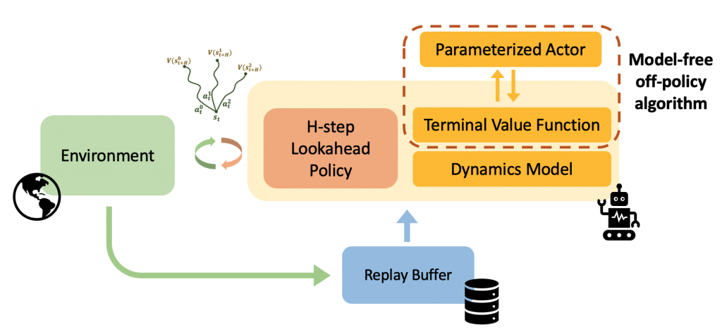
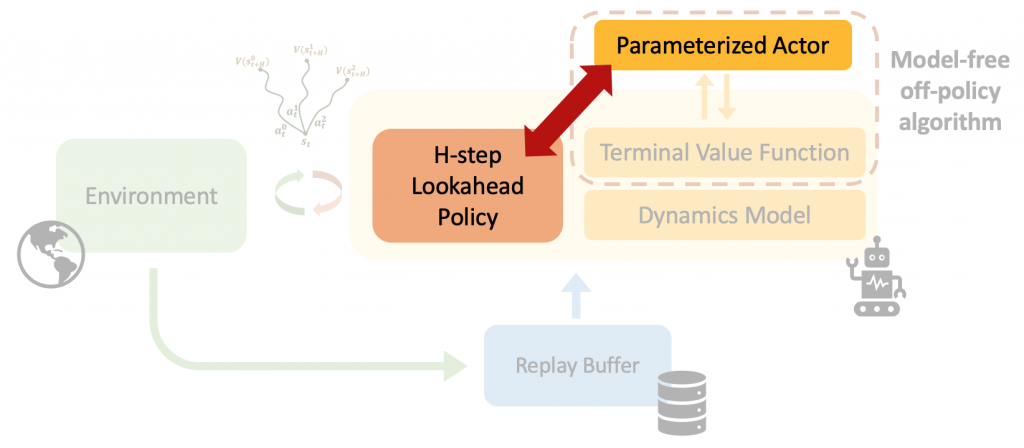
Figure 1. Overview of LOOP: Model-free Reinforcement Learning learns a policy by training a value function. In this setting, the performance of the policy is dependent on the accuracy of the learned value function. We propose LOOP, an efficient framework to learn with a policy that finds the best action sequence using imaginary rollouts with a learned model. This allows LOOP to potentially reduce dependence on value function errors. LOOP achieves strong performance across a range of tasks and problem settings.

Model-Free Off-Policy Reinforcement Learning

Reinforcement learning (RL) enables artificial agents to learn different tasks by interacting with the environment. Within RL, off-policy methods have brought about numerous successes recently for efficiently learning behaviors in applications such as robotics due to their ability to leverage previously collected data efficiently and incorporate data from a variety of sources.

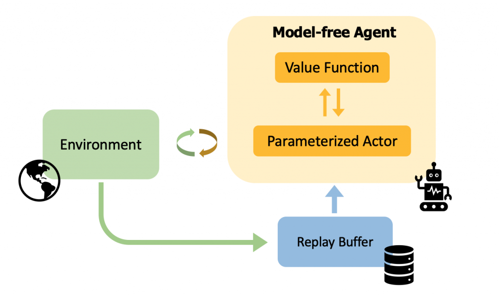
Figure 2. Illustration of a typical model-free reinforcement learning agent.

How does off-policy reinforcement learning work? A model-free off-policy reinforcement learning algorithm typically consists of a parameterized actor and a value function (see Figure 2). The actor interacts with the environment collecting the transitions in the replay buffer. The value function is trained using the transitions from the replay buffer to predict the cumulative return of the actor, and the actor is updated by maximizing the action-values at the states visited in the replay buffer. This framework suffers from the following issues:

  1. The performance of the actor is highly dependent on the accuracy of the learned value function. Learning an accurate value function is challenging in deep reinforcement learning with issues pointed out by previous works such as divergence, instability, rank loss, delusional bias and overestimation. 
  2. Traditionally in model-free RL methods, the parametrized actor is a neural network which is uninterpretable and inflexible in dealing with constraints during deployment. On the other hand, risk-sensitive domains such as healthcare or autonomous driving require us to reason about why the policy chose a particular action or incorporate safety constraints.

So, how should the actor choose actions if the value function is inaccurate? In this work, we suggest using a policy that looks ahead in the future using a learned model to find the best action sequence. This lookahead policy is more interpretable than the parametric actor and also allows us to incorporate constraints. Then we present a computationally efficient framework of learning with the lookahead policy that we call LOOP. We also show how LOOP can also be applied to the offline RL and safe RL along with the online RL setting.

H-step Lookahead Policy

In order to increase the performance, safety, and interpretability of reinforcement learning, we use online planning (“H-step lookahead”) with a terminal value function. In H-step lookahead, we use a learned dynamics model to roll out action sequences for H-horizon into the future and get the cumulative reward. To reason about the future reward beyond H steps, we attach a value function at the end of the rollout. The objective is to select the action sequence that will lead to rollout with the best cumulative return.

Stated formally, H-step lookahead objective aims to find an action sequence ((a_{0:H-1})) that maximizes the following objective:

$$max_{a_{0:H-1}} left[mathbb{E}_{hat{M}}[sum_{t=0}^{H-1}gamma^tr(s_t,a_t)+gamma^Hhat{V}(s_H)]right]$$

where (hat{M}) is the learned dynamics model, (hat{V}) is the learned terminal value function, (r) is the reward function and (gamma) is the discount factor.

H-step lookahead provides several benefits: 1. H-step lookahead reduces dependency on value function errors by using the model rollouts which allows it to trade-off value errors with model-errors. 2. H-step lookahead offers a degree of interpretability that is missing in fully parametric methods and 3. H-step lookahead allows the user to incorporate constraints (even non-stationary) and behavior priors during deployment. 

We can also provide theoretical guarantees that demonstrate using an H-step lookahead instead of a parametric actor (1-step greedy actor) can reduce dependency on value errors by a large margin while introducing a dependence on model errors. Despite the additional model errors, we argue that the H-step lookahead is useful as value errors can stem from several reasons as discussed in the previous section. In the low data regime, value errors can also stem from compounding sampling errors whereas the model can be expected to have smaller errors as it is trained with denser supervision using supervised learning. We hypothesize that these numerous sources of errors in value learning make the tradeoff of value-errors with model-errors beneficial and see empirical evidence for the same in our experiments.

LOOP: Learning Off-Policy with Online Planning

As described above, the H-step lookahead policy uses a terminal value function at the end of the H steps.  How do we learn the value function for this H-step lookahead policy?  The difficulty is that, in learning a value function, we need to evaluate the H-step lookahead policy from different states.  However, evaluating the H-step lookahead policy is somewhat slow (Lowrey et al.), since the lookahead policy requires simulating the dynamics for H-steps, which makes such an approach computationally expensive.

Figure 3. LOOP uses a parameterized actor instead of the H-step lookahead policy to learn the value function in a more computationally efficient manner.

Instead, we propose to learn a parameterized actor to more efficiently learn the terminal value function; to learn the value function, we can evaluate the actor (which is fast) instead of evaluating the H-step lookahead policy (which is slow).  We call this approach LOOP: Learning off-policy with online planning.  However, the problem with this approach is that there might be a difference between the H-step lookahead policy and the parametric actor (see Figure 3).  The difference between these policies can cause unstable learning, which we refer to as “actor divergence.” 

Figure 4. In LOOP, the H-step lookahead policy and the parameterized actor can be different policies causing unstable learning. We refer to this issue as “actor divergence”.

Our solution to actor divergence is to constrain the H-step lookahead policy based on the KL-divergence to a prior, where the prior is based on the parametric actor.  This constrained optimization helps ensure that the H-step lookahead policy remains similar to the parametric actor, leading to significantly more stable training. Specifically, we propose actor regularized control (ARC), which uses the following objective 

$$p^tau_{opt}=text{argmax}_{p^tau} mathbb{E}_{p^tau} left[mathbb{E}_{hat{M}}[R_{H,hat{V}}(s_t,tau)]right]~,~textrm{s.t}~~D_{KL}(p^tau||p^tau_{prior})le epsilon$$

The inner expectation estimates the return of the H-step lookahead (R_{H,hat{V}}) under model uncertainty while the outer expectation is under a distribution of action sequences.

In the above objective, we aim to find a distribution (p^tau=p^tau_{opt}) over the action sequence (tau) that maximizes the H-step lookahead return (R_{H,hat{V}}(s_t,tau)) while ensuring that the distribution of the action sequence is close to some predefined prior  (p^tau_{prior}). In ARC we set this prior to be equal to the parametrized actor and this ensures that H-step lookahead is close to the parametrized actor while still improving the cumulative return. This constrained optimization has a closed-form solution given by ( p^tau_{opt} propto p^tau_{prior} e^{frac{1}{eta}mathbb{E}_{hat{M}}[R_{H,hat{V}}(s_t,tau)]} ). Since the closed-form solution is unnormalized, we approximate it by a gaussian and improve the estimate of its mean and variance by iterative self-normalized importance sampling.

LOOP for Offline and Safe RL

In the previous section, we have seen that ARC optimizes for the expected return in the online RL setting.  LOOP can be extended to work in two other domains: 1. Offline RL: Learning from a fixed dataset of collected experience 2. Safe RL: Learning to maximize rewards which ensures that the constraint violations are below some threshold. 

For offline RL, ARC optimizes for the following underestimate of H-step lookahead return similar to previous offline RL methods ([1,2]).

$$text{mean}_{[K]}[R_{H,hat{V}}(s_t,tau)] – beta_{pess}text{std}_{[K]}[R_{H,hat{V}}(s_t,tau)]$$

where ([K]) denote model ensembles for uncertainty estimation and (beta_{pess}) is an hyperparameter.

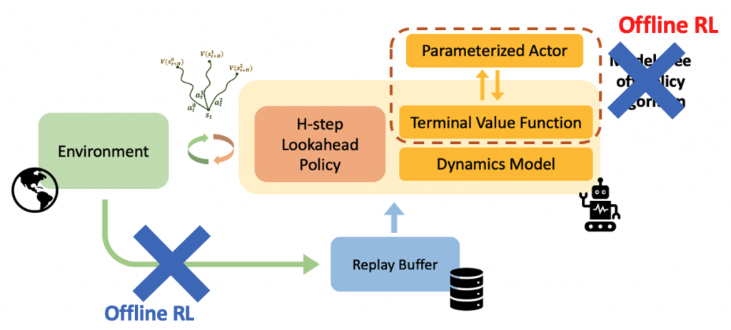
Figure 5. LOOP can be used for offline RL by using a fixed dataset of transitions and modifying ARC to optimize for underestimate of the expected return.

In this setting, the off-policy algorithm is also replaced by an offline RL algorithm (see Figure 5).

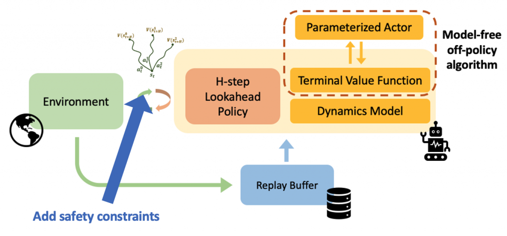
For safe RL, ARC optimizes for a constrained H-step lookahead objective which ensures that the cumulative constraint cost in the planning horizon are less than the predefined threshold (see Figure 6).

$$text{argmax}_{a_t} mathbb{E}_{hat{M}}[R_{H,hat{V}}(s_t,tau)]~~text{s.t}~max_{[K]}sum_{t=t}^{t+H-1}gamma^t c(s_t,a_t)le d_0$$

where (c) is the cost function.

Figure 6. LOOP can be used for safe RL by modifying ARC to optimize under safety constraints.

Experiments: Online, Offline, and Safe RL

Online RL: We use SAC as the off-policy algorithm in LOOP and test it on a set of MuJoCo locomotion and manipulation tasks. LOOP is compared against a variety of baselines covering model-free (SAC), model-based (PETS-restricted), and hybrid model-free+model-based (MBPO, LOOP-SARSA, SAC-VE) methods. LOOP-SARSA is a variant of LOOP that evaluates the replay buffer policy in its critic.

Figure 7. Learning performance comparison for online RL of LOOP-SAC to model-based and model-free baselines on the MuJoCo locomotion and manipulation tasks.

LOOP-SAC significantly improves performance over SAC, the underlying off-policy algorithm used to learn the terminal value function. The increase in efficiency over the SAC  empirically confirms that model-error tradeoff with value-error is indeed beneficial. LOOP-SAC is also competitive to MBPO in locomotion tasks, outperforming it significantly in manipulation tasks.

Figure 8. Environments used to compare the performance of LOOP to baselines. From left: Walker-v2, Ant-v2, PenGoal-v0, Claw-v1, PointGoal-v1

Offline RL: We combine LOOP with two offline RL methods Critic Regularized Regression (CRR) and Policy in latent action space (PLAS) and test it on D4RL datasets. LOOP improves over CRR and PLAS with an average improvement of 15.91% and 29.49% respectively on the D4RL locomotion datasets. This empirically demonstrates that H-step lookahead improves performance over a pre-trained value function (obtained from offline RL) by reducing dependence on value errors.

Safe RL: For testing the safety performance of LOOP we experiment on the OpenAI safety gym environments. In the two environments, CarGoal and PointGoal, the agent needs to navigate to a goal while avoiding obstacles. 

Figure 9. Comparison of constraint violations (left two plots) and cumulative return (right two plots) on OpenAI safety gym environments of safeLOOP compared to baselines.

SafeLOOP (Figure above) is the modification of LOOP with constrained H-step lookahead that incorporates constraints. safeLOOP can learn orders of magnitude faster while still being safer than safeRL baselines.

Next Steps

A benefit of using H-step lookahead for deployment is its ability to incorporate non-stationary exploration priors, as this framework disentangles the exploitation policy (parametrized actor) and the exploration policy (H-step lookahead) to a certain degree. Exploring how more principled exploration techniques can enable data collection that leads to better policy improvement is an interesting future direction.    

Learning with H-step lookahead efficiently is challenging and unscalable. In our work, we demonstrated one particular way to learn efficiently with H-step lookahead but our approach introduced the issue of actor divergence. Some open questions are 1. What are other ways to learn efficiently with an H-step lookahead policy that does not suffer from actor divergence? 2. How can the actor divergence be reduced without restricting the H-step lookahead policy to be near the parametrized policy (eg. Offline RL)?

Further reading

If you’re interested in more details, please check out the links to the full paper, the project website, talk, and more!

Citation

This blog post is based on the following paper (BibTeX) :

Harshit Sikchi, Wenxuan Zhou, and David Held.
Learning Off-Policy with Online Planning.
In Conference of Robot Learning, November 2021.

Acknowledgments

Thanks to Wenxuan Zhou, Ben Eysenbach, Paul Liang, and David Held for feedback on this post! This material is based upon work supported by the United States Air Force and DARPA under Contract No. FA8750-18-C-0092, LG Electronics and the National Science Foundation under Grant No. IIS-1849154.

Read More

Blur faces in videos automatically with Amazon Rekognition Video

With the advent of artificial intelligence (AI) and machine learning (ML), customers and the general public have become increasingly aware of their privacy, as well as the value that it holds in today’s data-driven world. Enterprises are actively seeking out and marketing privacy-first solutions, especially in the Computer Vision (CV) domain. They need to reassure their customers that personal information such as faces are anonymized and generally kept safe.

Face blurring is one of the best-known practices when anonymizing both images and videos. It usually involves first detecting the face in an image/video, then applying a blob of pixels or other distortion effects on it. This workload can be considered a CV task. First, we analyze the pixels of the image/video until a face is recognized, then we extract the area where the face is in every frame, and finally we apply a mask on the previously found pixels. The first part of this can be achieved with ML and Deep Learning tools, such as Amazon Rekognition, while the second part is standard pixel manipulation.

In this post, we demonstrate how AWS Step Functions can be used to orchestrate AWS Lambda functions that call Amazon Rekognition Video to detect faces in videos, and use an open source CV and ML software library called OpenCV to blur them.

Solution overview

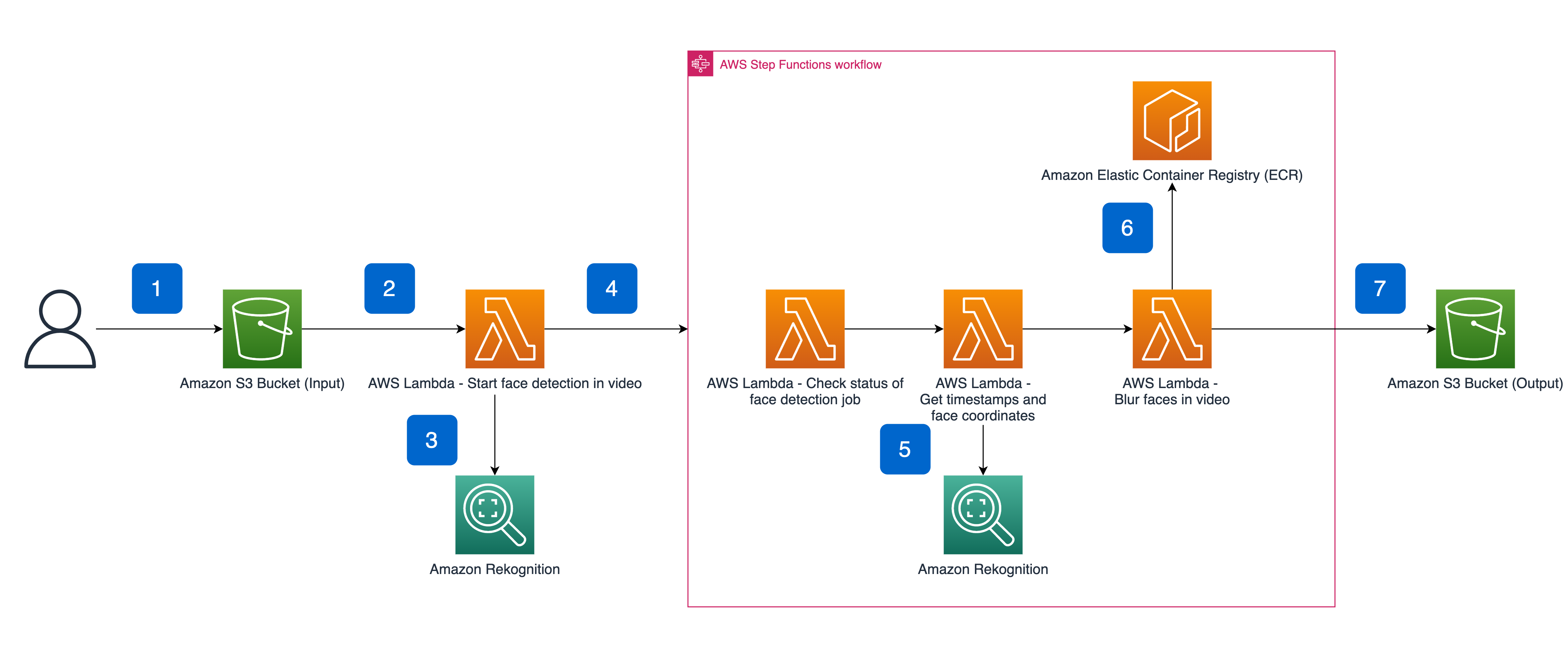
In our solution, AWS Step Functions, a low-code visual workflow service used to orchestrate AWS services, automate business processes, and build serverless applications, is used to orchestrate the calls and manage the flow of data between AWS Lambda functions. When an object is created in an Amazon Simple Storage Service (S3) bucket, for example by a video file upload, an ObjectCreated event is detected and a first Lambda function is triggered. This Lambda function makes an asynchronous call to the Amazon Rekognition Video face detection API and starts the execution of the AWS Step Functions workflow.

Inside the workflow, we use a Lambda function and a Wait State until the Amazon Rekognition Video asynchronous analysis started earlier finishes execution. Afterward, another Lambda function retrieves the result of the completed process from Amazon Rekognition and passes it to another Lambda function that uses OpenCV to blur the detected faces. To easily use OpenCV with our Lambda function, we built a Docker image hosted on Amazon Elastic Container Registry (ECR), and then deployed on AWS Lambda thanks to Container Image Support.

The architecture is entirely serverless, so we don’t need to provision, scale, or maintain our infrastructure. We also use Amazon Rekognition, a highly scalable and managed AWS AI service that requires no deep learning expertise.

Moreover, we have built our application with the AWS Cloud Development Kit (AWS CDK), an open-source software development framework. This lets us write Infrastructure as Code (IaC) using Python, thereby making the application easy to deploy, modify, and maintain.

Let’s look closer at the suggested architecture:

  1. The event flow starts at the moment of the video ingestion into Amazon S3. Amazon Rekognition Video supports MPEG-4 and MOV file formats, encoded using the H.264 codec.
  2. After the video file has been stored into Amazon S3, it automatically kicks-off an event triggering a Lambda function.
  3. The Lambda function uses the video’s attributes (name and location on Amazon S3) to start the face detection job on Amazon Rekognition through an API call.
  4. The same Lambda function then starts the Step Functions state machine, forwarding the video’s attributes and the Amazon Rekognition job ID.
  5. The Step Functions workflow starts with a Lambda function waiting for the Amazon Rekognition job to be finished. Once it’s done, another Lambda function gets the results from Amazon Rekognition.
  6. Finally, a Lambda function with Container Image Support fetches its Docker image, which supports OpenCV from Amazon ECR, blurs the faces detected by Amazon Rekognition, and temporarily stores the output video locally.
  7. Then, the blurred video is put into the output S3 bucket and removed from local files.

Providing a serverless function access to OpenCV is easier than ever with Container Image Support. Instead of uploading a code package to AWS Lambda, the function’s code resides in a Docker image that is hosted in Amazon Elastic Container Registry.

FROM public.ecr.aws/lambda/python:3.7
# Install the function's dependencies
# Copy file requirements.txt from your project folder and install
# the requirements in the app directory.
COPY requirements.txt  .
RUN  pip install -r requirements.txt
# Copy helper functions
COPY video_processor.py video_processor.py
# Copy handler function (from the local app directory)
COPY  app.py  .
# Overwrite the command by providing a different command directly in the template.
CMD ["app.lambda_function"]

If you want to build your own application using Amazon Rekognition face detection for videos and OpenCV to process videos with Python, consider the following:

  • Amazon Rekognition API responses for videos contain faces-detected timestamps in milliseconds
  • OpenCV works on frames and uses the video’s frame rate to combine frames into a video

Therefore, you must convert Amazon Rekognition information to make it usable with OpenCV. You may find our implementation in the apply_faces_to_video function, in /rekopoc-apply-faces-to-video-docker/video_processor.py.

Deploy the application

If you want to deploy the sample application to your own account, go to this GitHub repository. Clone it to your local environment (you can also use tools such as AWS Cloud9) and deploy it via cdk deploy. Find more details in the later section “Deploy the AWS CDK application”. First, let’s look at the repository project structure.

Project structure

This project contains source code and supporting files for a serverless application that you can deploy with the AWS CDK. It includes the following files and folders.

  • rekognition_video_face_blurring_cdk/ – CDK Python code for deploying the application.
  • rekopoc-apply-faces-to-video-docker/ – Code for Lambda function: uses OpenCV to blur faces per frame in video, uploads final result to output S3 bucket.
  • rekopoc-check-status/ – Code for Lambda function: Gets face detection results for the Amazon Rekognition Video analysis.
  • rekopoc-get-timestamps-faces/ – Code for Lambda function: Gets bounding boxes of detected faces and associated timestamps.
  • rekopoc-start-face-detect/ – Code for Lambda function: is triggered by an S3 event when a new .mp4 or .mov video file is uploaded, starts asynchronous detection of faces in a stored video, and starts the execution of AWS Step Functions’ State Machine.
  • requirements.txt – Required packages for deploying the AWS CDK application.

The application uses several AWS resources, including AWS Step Functions, Lambda functions, and S3 buckets. These resources are defined in the rekognition_video_face_blurring_cdk/rekognition_video_face_blurring_cdk_stack.py of this project. Update the Python code to add AWS resources through the same deployment process that updates your application code. Depending on the size of the video that you want to anonymize, you might need to update the configuration of the Lambda functions and adjust memory and timeout. You can provision a maximum of 10,240 MB (10 GB) of memory, and configure your AWS Lambda functions to run up to 15 minutes per execution.

Deploy the AWS CDK application

The AWS Cloud Development Kit (AWS CDK) is an open-source software development framework to define your cloud application resources using familiar programming languages. This project uses the AWS CDK in Python.

To build and deploy your application for the first time, you must:

Step 1: Ensure you have Docker running.
You will need Docker running to build the image before pushing it to Amazon ECR.

Step 2: Configure your AWS credentials.
The easiest way to satisfy this requirement is to issue the following command in your shell:

aws configure

For additional guidance on how to set up your AWS CLI installation, follow the Quick configuration with aws configure from the AWS CLI user guide.

Step 3: Install the AWS CDK and the requirements.
Simply run the following in your shell:

npm install -g aws-cdk
pip install -r requirements.txt
  • The first command will install the AWS CDK Toolkit globally using Node Package Manager.
  • The second command will install all of the Python packages needed by the AWS CDK using pip package manager. This command should be issued from the root folder of the cloned GitHub repository.

Step 4: Bootstrap your AWS environment for the CDK and deploy the application.

cdk bootstrap
cdk deploy
  • The first command will provision initial resources that the AWS CDK needs to perform the deployment. These resources include an Amazon S3 bucket for storing files and IAM roles that grant permissions needed to perform deployments.
  • Finally, cdk deploy will deploy the stack.

Step 5: Test the application.
Upload a video to the input S3 bucket through the AWS Management Console, the AWS CLI, or the SDK, and find the result in the output bucket.

Cleanup

To delete the sample application that you created, use the AWS CDK:

cdk destroy

Conclusion

In this post, we showed you how to deploy a solution to automatically blur videos without provisioning any resources to your AWS account. We used Amazon Rekognition Video face detection feature, Container Image Support for AWS Lambda functions to easily work with OpenCV, and we orchestrated the whole workflow with AWS Step Functions. Finally, we made our solution comprehensive and reusable with the AWS CDK to make it easier to deploy and adapt.

Next Steps

If you have feedback about this post, submit it in the Comments section below. For more information, visit the following links about the tools and services that we used and follow the code in GitHub. We look forward to your feedback and contributions!


About the Authors

Anastasia Pachni Tsitiridou is a Solutions Architect at AWS. She is based in Amsterdam and supports ISVs across the Benelux in their cloud journey. She studied Electrical and Computer Engineering before being introduced to Computer Vision. What she enjoys most nowadays is working at the intersection of CV and ML.

Olivier Sutter is a Solutions Architect in France. He is based in Paris and always sets his customers’ best interests as his top priority. With a strong academic background in applied mathematics, he started developing his AI/ML passion at university, and now thrives applying this knowledge on real-world use-cases with his customers.

Davide Gallitelli is a Specialist Solutions Architect for AI/ML in the EMEA region. He is based in Brussels and works closely with customer throughout Benelux. He has been a developer since very young, starting to code at the age of 7. He has started learning AI/ML since the latest years of university, and has fallen in love with it since then.

Read More

Scooping up Customers: Startup’s No-Code AI Gains Traction for Industrial Inspection

Bill Kish founded Ruckus Wireless two decades ago to make Wi-Fi networking easier. Now, he’s doing the same for computer vision in industrial AI.

In 2015, Kish started Cogniac, a company that offers a self-service computer vision platform and development support.

Like in the early days of Wi-Fi deployment, the rollout of AI is challenging, he said. Cogniac’s answer is to offer companies a fast track to building datasets on their own for models by scanning parts and equipment, using its no-code AI platform.

No-code AI platforms enable people to work with visual tools and user interfaces — for labeling data, for example — to help develop applications without any programming skill required.

It’s a strategy that’s working. Cogniac customers include Ford, freight giant BNSF Railway and tractor maker Doosan Bobcat. The startup turbocharges these businesses with NVIDIA GPUs for all training and inference.

Cogniac, based in Silicon Valley, recently landed a $20 million Series B investment. The company is an NVIDIA Metropolis partner and a member of NVIDIA Inception, a program that offers go-to-market support, expertise and technology for AI, data science and HPC startups. NVIDIA Metropolis is an application framework that makes it easier for developers to combine video cameras and sensors with AI-enabled video analytics.

BNSF Spots Railroad Damages

North America’s largest freight railway network, BNSF Railway has more than 32,000 miles of track in 28 U.S. states and more than 8,000 locomotives, a massive challenge for keeping up with inspections. BNSF relies on Cogniac to build models for inspections of train tracks, train wheels and other parts.

Cogniac enables BNSF to use mobile devices to gather images of defects that can be automatically fed into models. BNSF has about 200 convolutional neural networks in production and several times that under development with Cogniac, said Kish. They’re helping the railway look for missing cotter pins and bolts on cars, tankers that have been left open and hundreds of other safety-related inspections.

Using GPUs onboard trains, Cogniac’s AI enables ongoing inspections of railways to detect broken rails. It also helps prioritize maintenance. Previously, inspections required closing down tracks for about a day to scrutinize sections of it, he said.

“It’s a huge win for the railways to be able to inspect their assets as a part of their ongoing operations,” said Kish.

Ford Detects Sheet Metal Defects

Ford relies on Cogniac for real-time inspections of sheet metal used in F-150 trucks, the best-selling vehicle in North America. Body panels and inner door panels are made of stamped aluminum sheet metal that is pressed into different shapes using a stamping tool.

But those stamped panels can sometimes have defects such as small splits that need to be detected before installation into vehicles.

“Our edge computing is processing gigapixels using dozens of cameras to capture the contours of the surfaces, enabled by NVIDIA GPUs,” said Kish.

Doosan Bobcat Bulldozes Errors

Doosan Bobcat, a Korean maker of compact tractors, was having a lot of missing parts in the build kits it sent out for tractor orders.Those parts kits are built in Minnesota and then sent to North Dakota for assembly. Missing parts were a big problem that stalled output.

But now the tractor giant is aided by Cogniac’s vision pipelines to monitor parts kits the company puts together for building different configurations of its Bobcat tractors.

Before Cogniac, one-third of the kits that Doosan Bobcat put together for building tractors were incomplete or incorrect. Since implementing Cogniac, kit errors are now one out of 20,000, according to Doosan Bobcat.

“Chances are that there are going to be parts that are missing or wrong,” said Kish. “It’s money that’s not going out the door.”

The post Scooping up Customers: Startup’s No-Code AI Gains Traction for Industrial Inspection appeared first on The Official NVIDIA Blog.

Read More