The senior product manager leading hardware and software product development at the Center for Quantum Computing wants to make fault-tolerant quantum computing a reality.Read More
Everyone’s a PC Gamer This GFN Thursday
It’s never been easier to be a PC gamer.
GeForce NOW is your gateway into PC gaming. With the power of NVIDIA GeForce GPUs in the cloud, any gamer can stream titles from the top digital games stores — even on low-powered hardware.
Evolve to the PC gaming ranks this GFN Thursday and get ready for seven more games streaming from the GeForce NOW library this week, including PC exclusives like Dread Hunger.
Set Yourself Free
Thanks to GeForce NOW, more gamers than ever can experience what it means to play PC games at unbelievable quality, across nearly all devices.
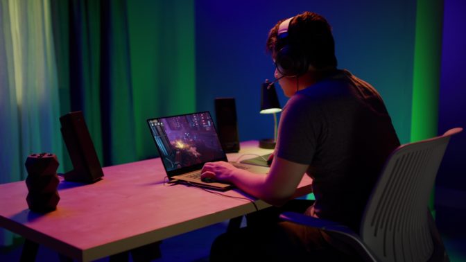
Members can stream over 1,000 PC titles that they own from digital game stores like Steam, Epic Games Store, Ubisoft Connect, Origin and GOG.com. And because they’re streaming from the cloud, nearly any of their devices can become a GeForce gaming rig — even Macs or mobile devices.
Playing PC games means getting access to an entire universe of PC exclusives — titles unavailable on other platforms. Unite and survive in Valheim, or battle for supremacy in Dota 2. Conquer the universe in EVE Online, or be the last one standing in Ring of Elysium. Join hundreds of players to explore New World, or squad up with other ghost hunters in Phasmophobia. The options are nearly endless.
Members on the RTX 3080 membership — now available in a 1-month option — can experience the next generation of cloud gaming, streaming gameplay on PC and Mac at up to 1440 pixels and 120 frames per second. And with support for NVIDIA DLSS and RTX ON, titles like Cyberpunk 2077 and Dying Light 2 are rendered at gorgeous cinematic quality — the way they were meant to be played.

New games join the GeForce NOW library every GFN Thursday, including the hottest PC titles like Dread Hunger, which pits you and seven others in a deadly game of survival and betrayal. Even with a small personal collection to start, instantly jump into nearly 100 free-to-play games from Steam and the Epic Games Store. All progress syncs with the cloud, so you can keep playing across your devices, or even on your own GeForce gaming rig.
Ready to join the PC universe? Sign up for a GeForce NOW membership, download the app or access the service directly from a supported browser and link game stores to your GeForce NOW library to start playing PC games across devices today.
Jump On In

There’s always something new to play on GeForce NOW. Here’s the complete list of seven titles coming this week:
- Monster Energy Supercross – The Official Videogame 5 (New release on Steam)
- Tunic (New release on Steam)
- Syberia: The World Before (New release on Steam and Epic Games Store, March 18)
- Blood West (Steam)
- Dread Hunger (Steam)
- Hero’s Hour (Steam)
- Hundred Days – Winemaking Simulator (Steam and Epic Games Store)
With the power of the cloud and all of these new games, we’ve got all that you need to be a PC gamer right here on Twitter:
it’s never been easier to become a PC gamer…
pic.twitter.com/qzjNbyYLRD
—
NVIDIA GeForce NOW (@NVIDIAGFN) March 16, 2022
The post Everyone’s a PC Gamer This GFN Thursday appeared first on NVIDIA Blog.
Amazon SageMaker JumpStart models and algorithms now available via API
In December 2020, AWS announced the general availability of Amazon SageMaker JumpStart, a capability of Amazon SageMaker that helps you quickly and easily get started with machine learning (ML). JumpStart provides one-click fine-tuning and deployment of a wide variety of pre-trained models across popular ML tasks, as well as a selection of end-to-end solutions that solve common business problems. These features remove the heavy lifting from each step of the ML process, making it easier to develop high-quality models and reducing time to deployment.
Previously, all JumpStart content was available only through Amazon SageMaker Studio, which provides a user-friendly graphical interface to interact with the feature. Today, we’re excited to announce the launch of easy-to-use JumpStart APIs as an extension of the SageMaker Python SDK. These APIs allow you to programmatically deploy and fine-tune a vast selection of JumpStart-supported pre-trained models on your own datasets. This launch unlocks the usage of JumpStart capabilities in your code workflows, MLOps pipelines, and anywhere else you’re interacting with SageMaker via SDK.
In this post, we provide an update on the current state of JumpStart’s capabilities and guide you through the usage flow of the JumpStart API with an example use case.
JumpStart overview
JumpStart is a multi-faceted product that includes different capabilities to help get you quickly started with ML on SageMaker. At the time of writing, JumpStart enables you to do the following:
- Deploy pre-trained models for common ML tasks – JumpStart enables you to solve common ML tasks with no development effort by providing easy deployment of models pre-trained on publicly available large datasets. The ML research community has put a large amount of effort into making a majority of recently developed models publicly available for use. JumpStart hosts a collection of over 300 models, spanning the 15 most popular ML tasks such as object detection, text classification, and text generation, making it easy for beginners to use them. These models are drawn from popular model hubs, such as TensorFlow, PyTorch, Hugging Face, and MXNet Hub.
- Fine-tune pre-trained models – JumpStart allows you to fine-tune pre-trained models with no need to write your own training algorithm. In ML, the ability to transfer the knowledge learned in one domain to another domain is called transfer learning. You can use transfer learning to produce accurate models on your smaller datasets, with much lower training costs than the ones involved in training the original model from scratch. JumpStart also includes popular training algorithms based on LightGBM, CatBoost, XGBoost, and Scikit-learn that you can train from scratch for tabular data regression and classification.
- Use pre-built solutions – JumpStart provides a set of 17 pre-built solutions for common ML use cases, such as demand forecasting and industrial and financial applications, which you can deploy with just a few clicks. The solutions are end-to-end ML applications that string together various AWS services to solve a particular business use case. They use AWS CloudFormation templates and reference architectures for quick deployment, which means they are fully customizable.
- Use notebook examples for SageMaker algorithms – SageMaker provides a suite of built-in algorithms to help data scientists and ML practitioners get started with training and deploying ML models quickly. JumpStart provides sample notebooks that you can use to quickly use these algorithms.
- Take advantage of training videos and blogs – JumpStart also provides numerous blog posts and videos that teach you how to use different functionalities within SageMaker.
JumpStart accepts custom VPC settings and KMS encryption keys, so that you can use the available models and solutions securely within your enterprise environment. You can pass your security settings to JumpStart within SageMaker Studio or through the SageMaker Python SDK.
JumpStart-supported ML tasks and API example Notebooks
JumpStart currently supports 15 of the most popular ML tasks; 13 of them are vision and NLP-based tasks, of which 8 support no-code fine-tuning. It also supports four popular algorithms for tabular data modeling. The tasks and links to their sample notebooks are summarized in the following table.
Depending on the task, the sample notebooks linked in the preceding table can guide you on all or a subset of the following processes:
- Select a JumpStart supported pre-trained model for your specific task.
- Host a pre-trained model, get predictions from it in real-time, and adequately display the results.
- Fine-tune a pre-trained model with your own selection of hyperparameters and deploy it for inference.
Fine-tune and deploy an object detection model with JumpStart APIs
In the following sections, we provide a step-by-step walkthrough of how to use the new JumpStart APIs on the representative task of object detection. We show how to use a pre-trained object detection model to identify objects from a predefined set of classes in an image with bounding boxes. Finally, we show how to fine-tune a pre-trained model on your own dataset to detect objects in images that are specific to your business needs, simply by bringing your own data. We provide an accompanying notebook for this walkthrough.
We walk through the following high-level steps:
- Run inference on the pre-trained model.
- Retrieve JumpStart artifacts and deploy an endpoint.
- Query the endpoint, parse the response, and display model predictions.
- Fine-tune the pre-trained model on your own dataset.
- Retrieve training artifacts.
- Run training.
Run inference on the pre-trained model
In this section, we choose an appropriate pre-trained model in JumpStart, deploy this model to a SageMaker endpoint, and show how to run inference on the deployed endpoint. All the steps are available in the accompanying Jupyter notebook.
Retrieve JumpStart artifacts and deploy an endpoint
SageMaker is a platform based on Docker containers. JumpStart uses the available framework-specific SageMaker Deep Learning Containers (DLCs). We fetch any additional packages, as well as scripts to handle training and inference for the selected task. Finally, the pre-trained model artifacts are separately fetched with model_uris, which provides flexibility to the platform. You can use any number of models pre-trained for the same task with a single training or inference script. See the following code:
Next, we feed the resources into a SageMaker Model instance and deploy an endpoint:
Endpoint deployment may take a few minutes to complete.
Query the endpoint, parse the response, and display predictions
To get inferences from a deployed model, an input image needs to be supplied in binary format along with an accept type. In JumpStart, you can define the number of bounding boxes returned. In the following code snippet, we predict ten bounding boxes per image by appending ;n_predictions=10 to Accept. To predict xx boxes, you can change it to ;n_predictions=xx , or get all the predicted boxes by omitting ;n_predictions=xx entirely.
The following code snippet gives you a glimpse of what object detection looks like. The probability predicted for each object class is visualized, along with its bounding box. We use the parse_response and display_predictions helper functions, which are defined in the accompanying notebook.
The following screenshot shows the output of an image with prediction labels and bounding boxes.
Fine-tune a pre-trained model on your own dataset
Existing object detection models in JumpStart are pre-trained either on the COCO or the VOC datasets. However, if you need to identify object classes that don’t exist in the original pre-training dataset, you have to fine-tune the model on a new dataset that includes these new object types. For example, if you need to identify kitchen utensils and run inference on a deployed pre-trained SSD model, the model doesn’t recognize any characteristics of the new image types and therefore the output is incorrect.
In this section, we demonstrate how easy it is to fine-tune a pre-trained model to detect new object classes using JumpStart APIs. The full code example with more details is available in the accompanying notebook.
Retrieve training artifacts
Training artifacts are similar to the inference artifacts discussed in the preceding section. Training requires a base Docker container, namely the MXNet container in the following example code. Any additional packages required for training are included with the training scripts in train_sourcer_uri. The pre-trained model and its parameters are packaged separately.
Run training
To run training, we simply feed the required artifacts along with some additional parameters to a SageMaker Estimator and call the .fit function:
While the algorithm trains, you can monitor its progress either in the SageMaker notebook where you’re running the code itself, or on Amazon CloudWatch. When training is complete, the fine-tuned model artifacts are uploaded to the Amazon Simple Storage Service (Amazon S3) output location specified in the training configuration. You can now deploy the model in the same manner as the pre-trained model. You can follow the rest of the process in the accompanying notebook.
Conclusion
In this post, we described the value of the newly released JumpStart APIs and how to use them. We provided links to 17 example notebooks for the different ML tasks supported in JumpStart, and walked you through the object detection notebook.
We look forward to hearing from you as you experiment with JumpStart.
About the Authors
 Dr. Vivek Madan is an Applied Scientist with the Amazon SageMaker JumpStart team. He got his PhD from University of Illinois at Urbana-Champaign and was a Post-Doctoral Researcher at Georgia Tech. He is an active researcher in machine learning and algorithm design, and has published papers in EMNLP, ICLR, COLT, FOCS, and SODA conferences.
 João Moura is an AI/ML Specialist Solutions Architect at Amazon Web Services. He is mostly focused on NLP use-cases and helping customers optimize Deep Learning model training and deployment.
 Dr. Ashish Khetan is a Senior Applied Scientist with Amazon SageMaker JumpStart and Amazon SageMaker built-in algorithms and helps develop machine learning algorithms. He is an active researcher in machine learning and statistical inference and has published many papers in NeurIPS, ICML, ICLR, JMLR, and ACL conferences.
How artificial intelligence can help combat systemic racism
In 2020, Detroit police arrested a Black man for shoplifting almost $4,000 worth of watches from an upscale boutique. He was handcuffed in front of his family and spent a night in lockup. After some questioning, however, it became clear that they had the wrong man. So why did they arrest him in the first place?
The reason: a facial recognition algorithm had matched the photo on his driver’s license to grainy security camera footage.
Facial recognition algorithms — which have repeatedly been demonstrated to be less accurate for people with darker skin — are just one example of how racial bias gets replicated within and perpetuated by emerging technologies.
“There’s an urgency as AI is used to make really high-stakes decisions,” says MLK Visiting Professor S. Craig Watkins, whose academic home for his time at MIT is the Institute for Data, Systems, and Society (IDSS). “The stakes are higher because new systems can replicate historical biases at scale.”
Watkins, a professor at the University of Texas at Austin and the founding director of the Institute for Media Innovation, researches the impacts of media and data-based systems on human behavior, with a specific concentration on issues related to systemic racism. “One of the fundamental questions of the work is: how do we build AI models that deal with systemic inequality more effectively?”
Ethical AI
Inequality is perpetuated by technology in many ways across many sectors. One broad domain is health care, where Watkins says inequity shows up in both quality of and access to care. The demand for mental health care, for example, far outstrips the capacity for services in the United States. That demand has been exacerbated by the pandemic, and access to care is harder for communities of color.
For Watkins, taking the bias out of the algorithm is just one component of building more ethical AI. He works also to develop tools and platforms that can address inequality outside of tech head-on. In the case of mental health access, this entails developing a tool to help mental health providers deliver care more efficiently.
“We are building a real-time data collection platform that looks at activities and behaviors and tries to identify patterns and contexts in which certain mental states emerge,” says Watkins. “The goal is to provide data-informed insights to care providers in order to deliver higher-impact services.”
Watkins is no stranger to the privacy concerns such an app would raise. He takes a user-centered approach to the development that is grounded in data ethics. “Data rights are a significant component,” he argues. “You have to give the user complete control over how their data is shared and used and what data a care provider sees. No one else has access.”
Combating systemic racism
Here at MIT, Watkins has joined the newly launched Initiative on Combatting Systemic Racism (ICSR), an IDSS research collaboration that brings together faculty and researchers from the MIT Stephen A. Schwarzman College of Computing and beyond. The aim of the ICSR is to develop and harness computational tools that can help effect structural and normative change toward racial equity.
The ICSR collaboration has separate project teams researching systemic racism in different sectors of society, including health care. Each of these “verticals” addresses different but interconnected issues, from sustainability to employment to gaming. Watkins is a part of two ICSR groups, policing and housing, that aim to better understand the processes that lead to discriminatory practices in both sectors. “Discrimination in housing contributes significantly to the racial wealth gap in the U.S.,” says Watkins.
The policing team examines patterns in how different populations get policed. “There is obviously a significant and charged history to policing and race in America,” says Watkins. “This is an attempt to understand, to identify patterns, and note regional differences.”
Watkins and the policing team are building models using data that details police interventions, responses, and race, among other variables. The ICSR is a good fit for this kind of research, says Watkins, who notes the interdisciplinary focus of both IDSS and the SCC.
“Systemic change requires a collaborative model and different expertise,” says Watkins. “We are trying to maximize influence and potential on the computational side, but we won’t get there with computation alone.”
Opportunities for change
Models can also predict outcomes, but Watkins is careful to point out that no algorithm alone will solve racial challenges.
“Models in my view can inform policy and strategy that we as humans have to create. Computational models can inform and generate knowledge, but that doesn’t equate with change.” It takes additional work — and additional expertise in policy and advocacy — to use knowledge and insights to strive toward progress.
One important lever of change, he argues, will be building a more AI-literate society through access to information and opportunities to understand AI and its impact in a more dynamic way. He hopes to see greater data rights and greater understanding of how societal systems impact our lives.
“I was inspired by the response of younger people to the murders of George Floyd and Breonna Taylor,” he says. “Their tragic deaths shine a bright light on the real-world implications of structural racism and has forced the broader society to pay more attention to this issue, which creates more opportunities for change.”
The science behind Hunches: Deep device embeddings
A machine learning model learns representations that cluster devices according to their usage patterns.Read More
Hybrid Quantum Algorithms for Quantum Monte Carlo
The intersection between the computational difficulty and practical importance of quantum chemistry challenges run on quantum computers has long been a focus for Google Quantum AI. We’ve experimentally simulated simple models of chemical bonding, high-temperature superconductivity, nanowires, and even exotic phases of matter such as time crystals on our Sycamore quantum processors. We’ve also developed algorithms suitable for the error-corrected quantum computers we aim to build, including the world’s most efficient algorithm for large-scale quantum computations of chemistry (in the usual way of formulating the problem) and a pioneering approach that allows for us to solve the same problem at an extremely high spatial resolution by encoding the position of the electrons differently.
Despite these successes, it is still more effective to use classical algorithms for studying quantum chemistry than the noisy quantum processors we have available today. However, when the laws of quantum mechanics are translated into programs that a classical computer can run, we often find that the amount of time or memory required scales very poorly with the size of the physical system to simulate.
Today, in collaboration with Dr. Joonho Lee and Professor David Reichmann at Colombia, we present the Nature publication “Unbiasing Fermionic Quantum Monte Carlo with a Quantum Computer”, where we propose and experimentally validate a new way of combining classical and quantum computation to study chemistry, which can replace a computationally-expensive subroutine in a powerful classical algorithm with a “cheaper”, noisy, calculation on a small quantum computer. To evaluate the performance of this hybrid quantum-classical approach, we applied this idea to perform the largest quantum computation of chemistry to date, using 16 qubits to study the forces experienced by two carbon atoms in a diamond crystal. Not only was this experiment four qubits larger than our earlier chemistry calculations on Sycamore, we were also able to use a more comprehensive description of the physics that fully incorporated the interactions between electrons.
 |
| Google’s Sycamore quantum processor. Photo Credit: Rocco Ceselin. |
A New Way of Combining Quantum and Classical
Our starting point was to use a family of Monte Carlo techniques (projector Monte Carlo, more on that below) to give us a useful description of the lowest energy state of a quantum mechanical system (like the two carbon atoms in a crystal mentioned above). However, even just storing a good description of a quantum state (the “wavefunction”) on a classical computer can be prohibitively expensive, let alone calculating one.
Projector Monte Carlo methods provide a way around this difficulty. Instead of writing down a full description of the state, we design a set of rules for generating a large number of oversimplified descriptions of the state (for example, lists of where each electron might be in space) whose average is a good approximation to the real ground state. The “projector” in projector Monte Carlo refers to how we design these rules — by continuously trying to filter out the incorrect answers using a mathematical process called projection, similar to how a silhouette is a projection of a three-dimensional object onto a two-dimensional surface.
Unfortunately, when it comes to chemistry or materials science, this idea isn’t enough to find the ground state on its own. Electrons belong to a class of particles known as fermions, which have a surprising quantum mechanical quirk to their behavior. When two identical fermions swap places, the quantum mechanical wavefunction (the mathematical description that tells us everything there is to know about them) picks up a minus sign. This minus sign gives rise to the famous Pauli exclusion principle (the fact that two fermions cannot occupy the same state). It can also cause projector Monte Carlo calculations to become inefficient or even break down completely. The usual resolution to this fermion sign problem involves tweaking the Monte Carlo algorithm to include some information from an approximation to the ground state. By using an approximation (even a crude one) to the lowest energy state as a guide, it is usually possible to avoid breakdowns and even obtain accurate estimates of the properties of the true ground state.
For the most challenging problems (such as modeling the breaking of chemical bonds), the computational cost of using an accurate enough initial guess on a classical computer can be too steep to afford, which led our collaborator Dr. Joonho Lee to ask if a quantum computer could help. We had already demonstrated in previous experiments that we can use our quantum computer to approximate the ground state of a quantum system. In these earlier experiments we aimed to measure quantities (such as the energy of the state) that are directly linked to physical properties (like the rate of a chemical reaction). In this new hybrid algorithm, we instead needed to make a very different kind of measurement: quantifying how far the states generated by the Monte Carlo algorithm on our classical computer are from those prepared on the quantum computer. Using some recently developed techniques, we were even able to do all of the measurements on the quantum computer before we ran the Monte Carlo algorithm, separating the quantum computer’s job from the classical computer’s.
This division of labor between the classical and the quantum computer helped us make good use of both resources. Using our Sycamore quantum processor, we prepared a kind of approximation to the ground state that would be difficult to scale up classically. With a few hours of time on the quantum device, we extracted all of the data we needed to run the Monte Carlo algorithm on the classical computer. Even though the data was noisy (like all present-day quantum computations), it had enough signal that it was able to guide the classical computer towards a very accurate reconstruction of the true ground state (shown in the figure below). In fact, we showed that even when we used a low-resolution approximation to the ground state on the quantum computer (just a few qubits encoding the position of the electrons), the classical computer could efficiently solve a much higher resolution version (with more realism about where the electrons can be).
Using our new hybrid quantum algorithm, we performed the largest ever quantum computation of chemistry or materials science. We used sixteen qubits to calculate the energy of two carbon atoms in a diamond crystal. This experiment was four qubits larger than our first chemistry calculations on Sycamore, we obtained more accurate results, and we were able to use a better model of the underlying physics. By guiding a powerful classical Monte Carlo calculation using data from our quantum computer, we performed these calculations in a way that was naturally robust to noise.
We’re optimistic about the promise of this new research direction and excited to tackle the challenge of scaling these kinds of calculations up towards the boundary of what we can do with classical computing, and even to the hard-to-study corners of the universe. We know the road ahead of us is long, but we’re excited to have another tool in our growing toolbox.
Acknowledgements
I’d like to thank my co-authors on the manuscript, Bryan O’Gorman, Nicholas Rubin, David Reichman, Ryan Babbush, and especially Joonho Lee for their many contributions, as well as Charles Neill and Pedram Rousham for their help executing the experiment. I’d also like to thank the larger Google Quantum AI team, who designed, built, programmed, and calibrated the Sycamore processor.
Learning to fly
Andrea Henshall, a retired major in the U.S. Air Force and current MIT PhD student, has completed seven tours of combat, two years of aerial circus performance, and three higher education degrees (so far). But throughout each step of her journey, all roads seemed to point to MIT.
Currently working on her doctoral degree with an MIT master’s already in her toolkit, she is quick to attribute her academic success to MIT’s open educational resources. “I kept coming back to MIT-produced open source learning,” she says. “MIT dominates in educational philanthropy when it comes to free high-quality learning sources.” To this day, Henshall recommends MIT OpenCourseWare (OCW) and MITx courses to students and her fellow veterans who are transitioning out of the service.
A love of flight and a drive to excel
Henshall first discovered OCW as she was pursuing her master’s degree in aeronautics and astronautics at MIT. Transitioning from an applied engineering program at the United States Air Force Academy to a more theoretical program proved a challenge for Henshall, and her first semester grades got her put on academic probation. During Independent Activities Period, she took Professor Gilbert Strang’s linear algebra courses on OCW, which included both videos and homework. Henshall found Strang very engaging and easy to learn from and found it helpful to work through the homework when they had the solutions available. She was able to lift her grades the following semester, and by the end of her program, she was getting all A’s. Henshall says, “OpenCourseWare really saved me. I was worried I wouldn’t be able to complete my master’s.”
Ever since Henshall learned the term “astronautical engineer” in the fourth grade, she knew what she wanted to be when she grew up. That early love of outer space and building things led her to a bachelor’s degree in astronautical engineering and the Air Force. There she served as a research and development officer, instructor pilot, and chief financial officer of her squadron. But a non-combat-related injury forced her to medically retire from being a pilot. “I was not doing well physically, and it was impossible for me to get hired to be a pilot outside of the Air Force.” After a brief detour as a part-time aerial circus performer, she decided to go back to school.
Learning how to learn
Working outside of academia for eight years proved to be a tough transition. Henshall says, “I had to translate the work I had done in the military into something relevant for an academic application, and the language they were looking for was very different from what I was used to.” She thought acquiring more recent academic work might help improve her application. She attended Auburn University for her second master’s degree (this time in computer science and software engineering) and started a PhD. Again she turned to MIT OCW to supplement her studies.
Henshall says, “I remembered vividly how much it had helped me in 2005, so of course that’s where I was going to start. Then I noticed that OCW linked to MITx, which had more interactive quizzes.” The OCW platform had also become more robust since she had first used it. “Back then, it was new, there wasn’t necessarily a standard,” she says. Over 10 years later, she found that most courses had more material, videos, and notes that more closely approximated an MIT course experience. Those additional open education resources gave Henshall an extra edge to complete a 21-month program in 12 months with a 4.0 GPA. Her advisor told her that she had the best thesis defense he had seen in 25 years.
In 2019, Henshall’s success helped her get accepted to MIT’s PhD program in the Department of Aeronautics and Astronautics, in the Autonomy and Embedded Robotics Accelerated (AERA) lab under the Laboratory for Information and Decision Systems (LIDS), with a Lester Durand Gardner Fellowship. Her focus is controls systems with a minor in quantum information. She says, “I’m literally living my dream. I’m at my dream school with my dream advisor.” Working with Professor Sertac Karaman in LIDS, Henshall plans to write her thesis on multi-agent reinforcement learning. But her relationship with online learning is far from over; again she has turned to OCW and MITx resources for the foundation to succeed in subjects such as controls, machine learning, quantum mechanics, and quantum computation.
When the pandemic struck the East Coast, Henshall was only nine months into her PhD program at MIT. The pivot to online learning made it difficult to continue building relationships with classmates. But what was a new course experience for many learners during the pandemic felt very familiar to Henshall. “I had a leg up because I already knew how to learn through prerecorded videos on a computer instead of three-dimensional human standing in front of a chalkboard. I had already learned how to learn.”
A lifelong commitment to service
Henshall plans to return to the Department of Defense or related industries. Currently, she works collaboratively on two major projects related to her PhD thesis and her career path after she completes the program. The first project is an AI accelerator program through the Air Force. Her work with unmanned aerial vehicles (a.k.a. drones) uses a small quadrotor to autonomously and quickly search a building using reinforcement learning. The primary intended use is search and rescue. The second project involves research into multi-agent reinforcement learning and pathfinding. While also intended for search and rescue, they could be used for a variety of non-emergency inspection purposes as well.
Henshall is eager to share open education resources. At Auburn she shared OCW materials with her classmates, and now she uses them with the students she tutors. She’s also committed to sharing knowledge and resources with her fellow service members, and is an active member of a number of veterans’ organizations. With the Warrior-Scholar Project, she answers questions from enlisted people going into undergraduate programs, ranging from “What’s parking like?” to “How did you prepare for school?” As a Service to School ambassador, she is assigned to mentor veterans who are transitioning out of the military and looking to apply to graduate school, usually MIT hopefuls or other competitive schools. She’s able to draw from her own application experience to help others identify the core message their application should communicate and finesse the language to sound less like a military brief and more like the “academic speak” they will encounter moving forward.
Henshall says, “My trajectory would be so different if MITx and OCW didn’t exist, and I feel that’s true for so many thousands of other students. So many other institutions have copied the model, but MIT was the first and it’s still the best.”
Running PyTorch Models on Jetson Nano
Overview
Nvidia Jetson Nano, part of the Jetson family of products or Jetson modules, is a small yet powerful Linux (Ubuntu) based embedded computer with 2/4GB GPU. With it, you can run many PyTorch models efficiently. This document summarizes our experience of running different deep learning models using 3 different mechanisms on Jetson Nano:
-
Jetson Inference the higher-level Nvidia API that has built-in support for running most common computer vision models which can be transfer-learned with PyTorch on the Jetson platform.
-
TensorRT a high-performance inference framework from Nvidia that requires the conversion of a PyTorch model to ONNX, and then to the TensorRT engine file that the TensorRT runtime can run.
-
PyTorch with the direct PyTorch API
torch.nnfor inference.
Setting up Jetson Nano
After purchasing a Jetson Nano here, simply follow the clear step-by-step instructions to download and write the Jetson Nano Developer Kit SD Card Image to a microSD card, and complete the setup. After the setup is done and the Nano is booted, you’ll see the standard Linux prompt along with the username and the Nano name used in the setup.
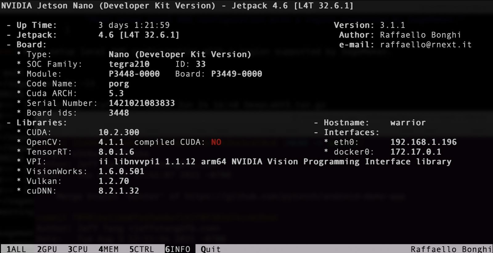
To check the GPU status on Nano, run the following commands:
sudo pip3 install jetson-stats
sudo jtop
You’ll see information, including:
You can also see the installed CUDA version:
$ ls -lt /usr/local
lrwxrwxrwx  1 root root   22 Aug  2 01:47 cuda -> /etc/alternatives/cuda
lrwxrwxrwx  1 root root   25 Aug  2 01:47 cuda-10 -> /etc/alternatives/cuda-10
drwxr-xr-x 12 root root 4096 Aug  2 01:47 cuda-10.2
To use a camera on Jetson Nano, for example, Arducam 8MP IMX219, follow the instructions here or run the commands below after installing a camera module:
cd ~
wget https://github.com/ArduCAM/MIPI_Camera/releases/download/v0.0.3/install_full.sh
chmod +x install_full.sh
./install_full.sh -m arducam
Another way to do this is to use the original Jetson Nano camera driver:
sudo dpkg -r arducam-nvidia-l4t-kernel
sudo shutdown -r now
Then, use ls /dev/video0 to confirm the camera is found:
$ ls /dev/video0
/dev/video0
And finally, the following command to see the camera in action:
nvgstcapture-1.0 --orientation=2
Using Jetson Inference
Nvidia Jetson Inference API offers the easiest way to run image recognition, object detection, semantic segmentation, and pose estimation models on Jetson Nano. Jetson Inference has TensorRT built-in, so it’s very fast.
To test run Jetson Inference, first clone the repo and download the models:
git clone --recursive https://github.com/dusty-nv/jetson-inference
cd jetson-inference
Then use the pre-built Docker Container that already has PyTorch installed to test run the models:
docker/run.sh --volume ~/jetson_inference:/jetson_inference
To run image recognition, object detection, semantic segmentation, and pose estimation models on test images, use the following:
cd build/aarch64/bin
./imagenet.py images/jellyfish.jpg /jetson_inference/jellyfish.jpg
./segnet.py images/dog.jpg /jetson_inference/dog.jpeg
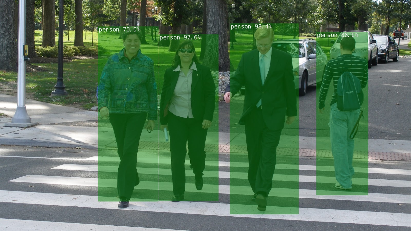
./detectnet.py images/peds_0.jpg /jetson_inference/peds_0.jpg
./posenet.py images/humans_0.jpg /jetson_inference/pose_humans_0.jpg
Four result images from running the four different models will be generated. Exit the docker image to see them:
$ ls -lt ~/jetson_inference/
-rw-r--r-- 1 root root  68834 Oct 15 21:30 pose_humans_0.jpg
-rw-r--r-- 1 root root 914058 Oct 15 21:30 peds_0.jpg
-rw-r--r-- 1 root root 666239 Oct 15 21:30 dog.jpeg
-rw-r--r-- 1 root root 179760 Oct 15 21:29 jellyfish.jpg



You can also use the docker image to run PyTorch models because the image has PyTorch, torchvision and torchaudio installed:
# pip list|grep torch
torch (1.9.0)
torchaudio (0.9.0a0+33b2469)
torchvision (0.10.0a0+300a8a4)
Although Jetson Inference includes models already converted to the TensorRT engine file format, you can fine-tune the models by following the steps in Transfer Learning with PyTorch (for Jetson Inference) here.
Using TensorRT
TensorRT is a high-performance inference framework from Nvidia. Jetson Nano supports TensorRT via the Jetpack SDK, included in the SD Card image used to set up Jetson Nano. To confirm that TensorRT is already installed in Nano, run dpkg -l|grep -i tensorrt:

Theoretically, TensorRT can be used to “take a trained PyTorch model and optimize it to run more efficiently during inference on an NVIDIA GPU.” Follow the instructions and code in the notebook to see how to use PyTorch with TensorRT through ONNX on a torchvision Resnet50 model:
-
How to convert the model from PyTorch to ONNX;
-
How to convert the ONNX model to a TensorRT engine file;
-
How to run the engine file with the TensorRT runtime for performance improvement: inference time improved from the original 31.5ms/19.4ms (FP32/FP16 precision) to 6.28ms (TensorRT).
You can replace the Resnet50 model in the notebook code with another PyTorch model, go through the conversion process above, and run the finally converted model TensorRT engine file with the TensorRT runtime to see the optimized performance. But be aware that due to the Nano GPU memory size, models larger than 100MB are likely to fail to run, with the following error information:
Error Code 1: Cuda Runtime (all CUDA-capable devices are busy or unavailable)
You may also see an error when converting a PyTorch model to ONNX model, which may be fixed by replacing:
torch.onnx.export(resnet50, dummy_input, "resnet50_pytorch.onnx", verbose=False)
with:
torch.onnx.export(model, dummy_input, "deeplabv3_pytorch.onnx", opset_version=11, verbose=False)
Using PyTorch
First, to download and install PyTorch 1.9 on Nano, run the following commands (see here for more information):
wget https://nvidia.box.com/shared/static/p57jwntv436lfrd78inwl7iml6p13fzh.whl -O torch-1.8.0-cp36-cp36m-linux_aarch64.whl -O torch-1.9.0-cp36-cp36m-linux_aarch64.whl
sudo apt-get install python3-pip libopenblas-base libopenmpi-dev
pip3 install Cython
pip3 install numpy torch-1.9.0-cp36-cp36m-linux_aarch64.whl
To download and install torchvision 0.10 on Nano, run the commands below:
https://drive.google.com/uc?id=1tU6YlPjrP605j4z8PMnqwCSoP6sSC91Z
pip3 install torchvision-0.10.0a0+300a8a4-cp36-cp36m-linux_aarch64.whl
After the steps above, run this to confirm:
$ pip3 list|grep torch
torch (1.9.0)
torchvision (0.10.0)
You can also use the docker image described in the section Using Jetson Inference (which also has PyTorch and torchvision installed), to skip the manual steps above.
The official YOLOv5 repo is used to run the PyTorch YOLOv5 model on Jetson Nano. After logging in to Jetson Nano, follow the steps below:
- Get the repo and install what’s required:
git clone https://github.com/ultralytics/yolov5
cd yolov5
pip install -r requirements.txt
- Run
python3 detect.py, which by default uses the PyTorch yolov5s.pt model. You should see something like:
detect: weights=yolov5s.pt, source=data/images, imgsz=[640, 640], conf_thres=0.25, iou_thres=0.45, max_det=1000, device=, view_img=False, save_txt=False, save_conf=False, save_crop=False, nosave=False, classes=None, agnostic_nms=False, augment=False, visualize=False, update=False, project=runs/detect, name=exp, exist_ok=False, line_thickness=3, hide_labels=False, hide_conf=False, half=False
YOLOv5 🚀 v5.0-499-g48b00db torch 1.9.0 CUDA:0 (NVIDIA Tegra X1, 3956.1015625MB)

Fusing layers...
Model Summary: 224 layers, 7266973 parameters, 0 gradients
image 1/5 /home/jeff/repos/yolov5-new/yolov5/data/images/bus.jpg: 640x480 4 persons, 1 bus, 1 fire hydrant, Done. (0.142s)
...
The inference time on Jetson Nano GPU is about 140ms, more than twice as fast as the inference time on iOS or Android (about 330ms).
If you get an error “ImportError: The _imagingft C module is not installed.” then you need to reinstall pillow:
sudo apt-get install libpng-dev
sudo apt-get install libfreetype6-dev
pip3 uninstall pillow
pip3 install --no-cache-dir pillow
After successfully completing the python3 detect.py run, the object detection results of the test images located in data/images will be in the runs/detect/exp directory. To test the detection with a live webcam instead of local images, use the --source 0 parameter when running python3 detect.py):
~/repos/yolov5$ ls -lt runs/detect/exp10
total 1456
-rw-rw-r-- 1 jeff jeff 254895 Oct 15 16:12 zidane.jpg
-rw-rw-r-- 1 jeff jeff 202674 Oct 15 16:12 test3.png
-rw-rw-r-- 1 jeff jeff 217117 Oct 15 16:12 test2.jpg
-rw-rw-r-- 1 jeff jeff 305826 Oct 15 16:12 test1.png
-rw-rw-r-- 1 jeff jeff 495760 Oct 15 16:12 bus.jpg
Using the same test files used in the PyTorch iOS YOLOv5 demo app or Android YOLOv5 demo app, you can compare the results generated with running the YOLOv5 PyTorch model on mobile devices and Jetson Nano:
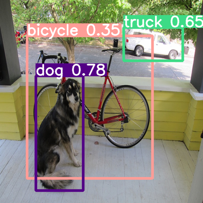
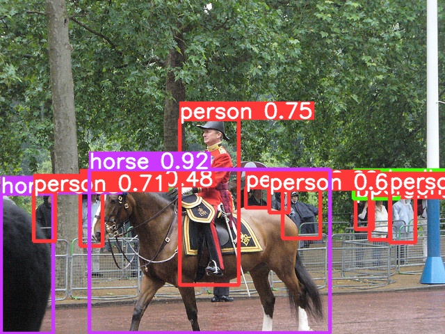
Figure 1. PyTorch YOLOv5 on Jetson Nano.
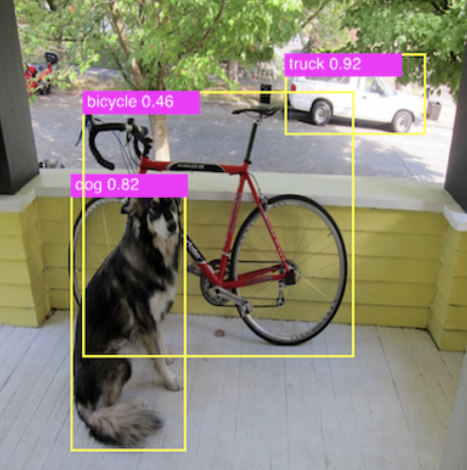
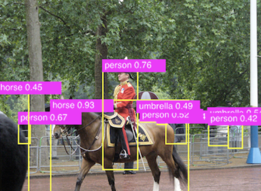
Figure 2. PyTorch YOLOv5 on iOS.
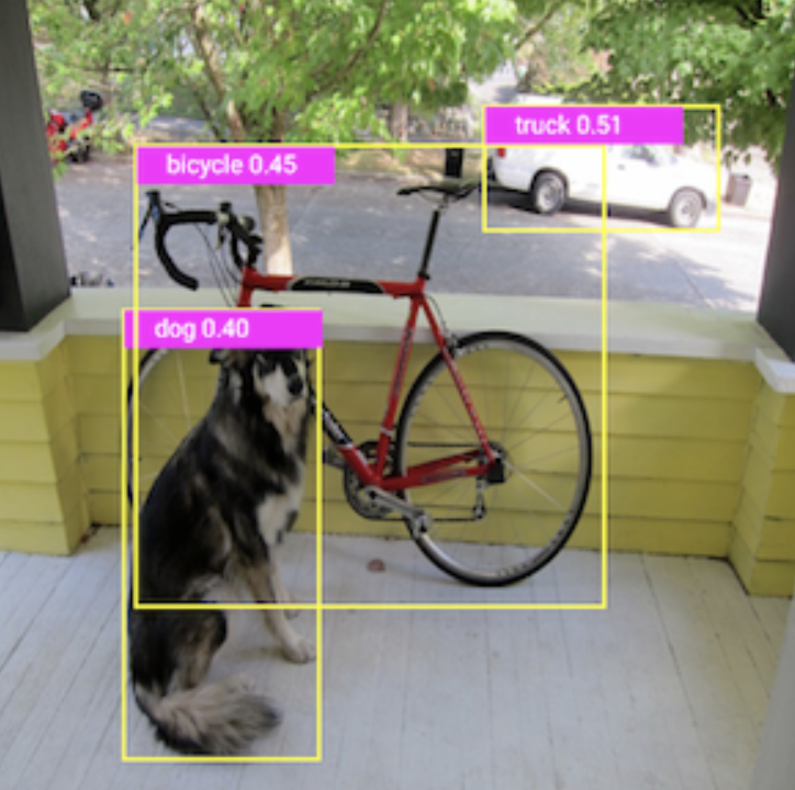
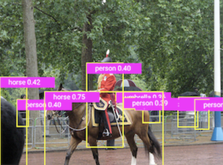
Figure 3. PyTorch YOLOv5 on Android.
Summary
Based on our experience of running different PyTorch models for potential demo apps on Jetson Nano, we see that even Jetson Nano, a lower-end of the Jetson family of products, provides a powerful GPU and embedded system that can directly run some of the latest PyTorch models, pre-trained or transfer learned, efficiently.
Building PyTorch demo apps on Jetson Nano can be similar to building PyTorch apps on Linux, but you can also choose to use TensorRT after converting the PyTorch models to the TensorRT engine file format.
But if you just need to run some common computer vision models on Jetson Nano using Nvidia’s Jetson Inference which supports image recognition, object detection, semantic segmentation, and pose estimation models, then this is the easiest way.
References
Torch-TensorRT, a compiler for PyTorch via TensorRT:
https://github.com/NVIDIA/Torch-TensorRT/
Jetson Inference docker image details:
https://github.com/dusty-nv/jetson-inference/blob/master/docs/aux-docker.md
A guide to using TensorRT on the Nvidia Jetson Nano:
https://docs.donkeycar.com/guide/robot_sbc/tensorrt_jetson_nano/
including:
-
Use Jetson as a portable GPU device to run an NN chess engine model:
https://medium.com/@ezchess/jetson-lc0-running-leela-chess-zero-on-nvidia-jetson-a-portable-gpu-device-a213afc9c018 -
A MaskEraser app using PyTorch and torchvision, installed directly with pip:
https://github.com/INTEC-ATI/MaskEraser#install-pytorch
A PyTorch to TensorRT converter:
https://github.com/NVIDIA-AI-IOT/torch2trt
The Google.org grantee using AI to detect bushfire risks
From predicting floods to improving waste management, organizations and researchers across Asia Pacific are using technology to respond to the impact of climate change.
Supporting this important work is a priority for Google.org. At today’s Southeast Asia Development Symposium, we announced a $6 million Sustainability Seed Fund to help organizations dedicated to addressing some of the region’s most difficult sustainability challenges. We look forward to sharing more in the coming weeks, including how nonprofits can apply.
The new fund builds on the support Google.org has already provided — through grants, technology and Googlers’ time — for sustainability-focused organizations and researchers across Asia-Pacific over recent years. I recently had the chance to talk to one of those existing grantees, Professor Hamish McGrowan from the University of Queensland in Australia, who received $1 million in Google.org support in 2021. Professor McGrowan and his team are working on a world-first hazard detection system for bushfires. It’s a powerful example of technology’s potential to protect communities in the short term and inform planning over the long term. It’s also part of Google’s Digital Future Initiative to propel Australian innovation and help Australians solve pressing problems.
Here’s what I learned from our conversation.
We know that bushfires have been a persistent issue in Australia. Could you give us a sense of the environmental challenges you’re seeing and how big this issue is?
Tackling bushfires is a nationwide issue. The Australian landscape has always been subject to fire, including what we may term nowadays as catastrophic fires. For example, many of Australia’s plants have evolved to require fire to germinate.
However, as the climate has changed in response to both natural and anthropogenic causes — and as urban areas expand into bushland — fire incidence has increased and arguably the scale and intensity of fires have too. One of the great challenges is managing and mitigating risk from bushfires in response to climate and land-use change and pollution pressures.
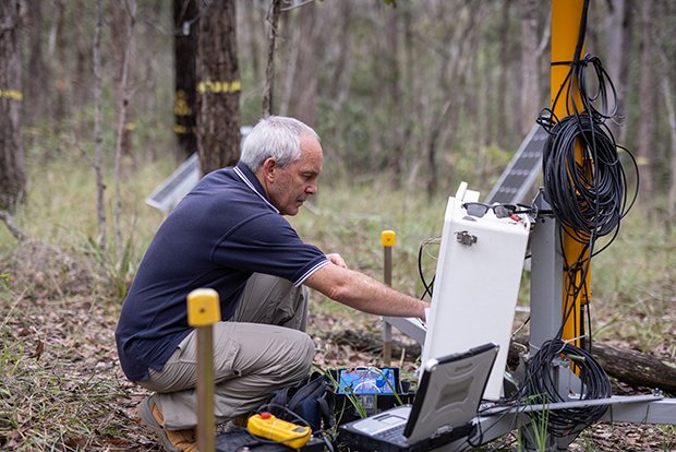
Professor Hamish testing out the solution
Could you share more about the solution you and your team have created to address the bushfires?
Over the past few years, my graduate students and I have developed a mobile weather radar capability with the support of generous industry organizations, including Google. Initially, the radar was used to study severe thunderstorms in southeast Queensland. We then tested the radar’s ability to observe bushfires and their interactions with the atmosphere. With the assistance of the radar’s manufacturer, Furuno Electric Co from Japan, we have now developed the capability to use the radar to identify and monitor meteorological hazards associated with severe bushfires — such as extreme winds, vortices, or burning embers. We are now developing this capacity further by applying artificial intelligence (AI) to near-real-time analysis of the radar data — so we can produce nowcasts of bushfire-related hazards.
I’m glad that through Google.org, we’ve been able to support the University of Queensland along the way. What do you hope to achieve with the new solution?
Our work ultimately aims to provide increased accuracy in forecasting bushfire movements and alerting community members and emergency responders before they spread. The $1 million grant from Google.org will enable our researchers to work on a new capability to identify and forewarn people in locations up to 30 kilometers downwind from the fire front that may come under attack from embers – sometimes in areas previously perceived as safe. Right now, we’re in the process of preparing for our first season of data collection using the mobile radar and have appointed new staff to the project.
From your perspective, how important are partnerships and support from governments, businesses, and communities in developing technology solutions?
Extremely important! We’ve long worked closely with local governments and various other organizations in areas of research and development. There are plenty of opportunities for collaboration and it’s wonderful to hear that Google.org is launching a new fund to support this kind of work across Asia Pacific.
What do you aspire to achieve with this solution in the next 10 years?
We hope to have a new bushfire warning capability that can be applied globally to save lives, businesses, and the environment from the perils of extreme bushfires and their interactions with the atmosphere.
GopherCite: Teaching language models to support answers with verified quotes
Language models like Gopher can “hallucinate” facts that appear plausible but are actually fake. Those who are familiar with this problem know to do their own fact-checking, rather than trusting what language models say. Those who are not, may end up believing something that isn’t true. This paper describes GopherCite, a model which aims to address the problem of language model hallucination. GopherCite attempts to back up all of its factual claims with evidence from the web.Read More


