Monthly Archives: March 2022

In this post, we will demonstrate how to securely launch notebook instances in a private subnet of an Amazon Virtual Private Cloud (Amazon VPC), with internet access disabled, and to securely connect to Amazon Simple Storage Service (Amazon S3) using VPC endpoints. This post is for network and security architects that support decentralized data science teams on AWS.

SageMaker notebook instances can be deployed in a private subnet and we recommend deploying them without internet access. Securing your notebook instances within a private subnet helps prevent unauthorized internet access to your notebook instances, which may contain sensitive information.

The examples in this post will use Notebook instance Lifecycle Configurations (LCCs) to connect to an S3 VPC endpoint and download idle-usage detection and termination scripts onto the notebook instance. These scripts are configured to be run as cron jobs, thus helping to save costs by automatically stopping idle capacity.

Solution overview

The following diagram describes the solution we implement. We create a SageMaker notebook instance in a private subnet of a VPC. We attach to that notebook instance a lifecycle configuration that copies an idle-shutdown script from Amazon S3 to the notebook instance at boot time (when starting a stopped notebook instance). The lifecycle configuration accesses the S3 bucket via AWS PrivateLink.

This architecture allows our internet-disabled SageMaker notebook instance to access S3 files, without traversing the public internet. Because the network traffic does not traverse the public internet, we significantly reduce the number of vectors bad actors can exploit in order to compromise the security posture of the notebook instance.

Prerequisites

We assume you have an AWS account, in addition to an Amazon VPC with at least one private subnet that is isolated from the internet. If you do not know how to create a VPC with a public/private subnet, check out this guide. A subnet is isolated from the internet if its route table doesn’t forward traffic to the internet through the NAT gateway and Internet gateway to the internet. The following screenshot shows an example of an isolated route table. Traffic stays within the subnet; there are no NAT gateways or internet gateways that could forward traffic to the internet.

Additionally, we need an S3 bucket. Any S3 bucket with the secure default configuration settings can work. Make sure you have read and write access to this bucket from the user account. This is important when we test our solution.  This entry in the S3 User Guide should clarify how to do this.

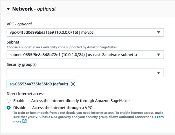
Now we create a SageMaker notebook instance. The notebook instance should be deployed into an isolated subnet with Direct Internet Access selected as Disabled.

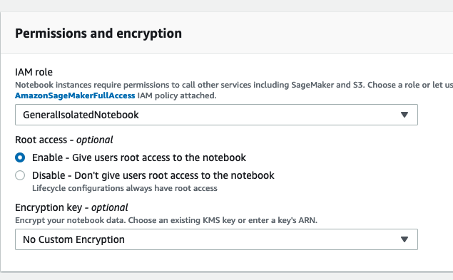
We also need to configure this notebook to run as the root user. Under Permissions and encryption, choose Enable for the Root access setting.

Once these settings have been configured, choose Create notebook instance at the bottom of the window.

Configure access to Amazon S3

To configure access to Amazon S3, complete the following steps:

1. On the Amazon S3 console, navigate to the S3 bucket you use to store scripts.

Access to objects in this bucket is only granted if explicitly allowed via an AWS Identity and Access Management (IAM) policy.

2. In this bucket, create a folder called lifecycle-configurations.
3. Copy the following script from GitHub and save it in your S3 bucket with the key lifecycle-configurations/autostop.py.

We can now begin modifying our network to allow access between Amazon S3 and our isolated notebook instance.

4. Write a least privilege IAM policy defining access to this bucket and the lifecycle policy script.
5. Create an AWS PrivateLink gateway endpoint to Amazon S3.
6. Create a SageMaker lifecycle configuration that requests the autostop.py script from Amazon S3 via an API call.
7. Attach the lifecycle configuration to the notebook instance.

After you implement these steps, we can test the configuration by performing an Amazon S3 CLI command in a notebook cell. If the command is successful, we have successfully implemented least privilege access to Amazon S3 from an isolated network location with AWS PrivateLink.

A more robust test would be to leave the notebook instance idle and allow the lifecycle policy to run as expected. If all goes well, the notebook instance should shut down after a 5-minute idle period.

Configure AWS PrivateLink for Amazon S3

AWS PrivateLink is a networking service that creates private endpoints in your VPC for other AWS services like Amazon Elastic Compute Cloud (Amazon EC2), Amazon S3, and Amazon Simple Notification Service (Amazon SNS). These endpoints facilitate API requests to other AWS services through your VPC instead of through the public internet. This is the crucial component that allows our solution to privately and securely access the S3 bucket that contains our lifecycle configuration script.

1. On the Amazon VPC console, choose Endpoints.

The list of endpoints is empty by default.

2. Choose Create endpoint.
3. For Service category, select AWS services.
4. For Service Name, search for S3 and select the gateway option.
5. For VPC, choose whichever private subnets you created earlier.
6. For Configure route tables, select the default route table for that VPC.
7. Under Policy, select the Custom option and enter the following policy code:

{
  "Version": "2008-10-17",
  "Statement": [
    {
      "Effect": "Allow",
      "Principal": "*",
      "Action": [
        "s3:Get*",
        "s3:List*"
      ],
      "Resource": [
        "arn:aws:s3:::<bucket-name>",
        "arn:aws:s3:::<bucket-name>/lifecycle-configurations/*"
      ]
    }
  ]
}

This policy document allows read-only access to the lifecycle-configurations S3 buckets. This policy restricts S3 operations to only the lifecycle-configurations bucket, we can additional buckets to the resource clause as we need. Although this endpoint’s policy isn’t least privilege access for our notebook instance, it still protects our S3 bucket resources from being modified by resources in this VPC.

8. To create this endpoint with the AWS CLI, run the following command:

aws ec2 create-vpc-endpoint --vpc-endpoint-type Gateway --vpc-id vpc-id --service-name com.amazonaws.region.s3 --route-table-ids route-table-id --policy-document 
'{
    "Version": "2008-10-17",
    "Statement": [
      {
        "Effect": "Allow",
        "PrincipalGroup": "*",
        "Action": [
          "s3:Get*",
          "s3:List*"
        ],
        "Resource": [
          "arn:aws:s3:::<bucket-name>",
          "arn:aws:s3:::<bucket-name>/lifecycle-configurations/*"
        ]
      }
   ]
}'

Gateway endpoints automatically modify the specified route tables to route traffic through to this endpoint. Although a route has been added, our VPC is still isolated. The route points to a managed prefix list, or a list of predefined IP addresses, used by the endpoint service to route traffic through this VPC to the Amazon S3 PrivateLink endpoint.

Modify the SageMaker notebook instance IAM role

We start by crafting a least privilege IAM policy for our notebook instance role’s policy document.

1. On the IAM console, choose Policies.
2. Choose Create policy.
3. On the JSON tab, enter the following code:

{
  "Version": "2012-10-17",
  "Statement": [
    {
      "Sid": "S3LifecycleConfigurationReadPolicy",
      "Effect": "Allow",
      "Action": [
        "s3:GetObject",
        "s3:ListBucket"
      ],
      "Resource": [
        "arn:aws:s3:::<bucket-name>",
        "arn:aws:s3:::<bucket-name>/lifecycle-configurations/*"
      ]
    }
  ]
}

This policy is an example of least privilege access, a security paradigm that is foundational to a Zero Trust architecture. This policy allows requests for GetObject and ListBucket API calls only, specifically on the Amazon S3 resources that manage our lifecycle policies. This IAM policy document can only be applied in instances where you’re downloading lifecycle policies from Amazon S3.

4. Save this policy as S3LifecycleConfigurationReadPolicy.
5. In the navigation pane, choose Roles.
6. Search for and choose the role attached to the isolated notebook instances and edit the role’s policy document.
7. Search for the newly created policy and attach it to this role’s policy document.

Now your isolated notebook has permissions to access Amazon S3 via the GetObject and ListBucket API calls. We can test this by running the following snippet in a notebook cell:

!aws s3api get-object --bucket <bucket-name> --key lifecycle-configurations/autostop.py autostop.py

At this point in the configuration, you should no longer see a permission denied error, but a timeout error. This is good; it means we have permission to access Amazon S3 but we haven’t established the network connectivity to do so. We do this in the next section.

Next, we create our IAM policy and role via the AWS Command Line Interface (AWS CLI).

8. Create the following policy and save the ARN from the output for a later step:

aws iam create-policy --policy-name S3LifecycleConfigurationReadPolicy --policy-document 
> '{
  "Version": "2012-10-17",
  "Statement": [
    {
      "Sid": "S3LifecycleConfigurationReadPolicy",
      "Effect": "Allow",
      "Action": [
        "s3:GetObject",
        "s3:ListBucket"
      ],
      "Resource": [
        "arn:aws:s3:::<bucket-name>",
        "arn:aws:s3:::<bucket-name>/lifecycle-configurations/*"
      ]
    }
  ]
}'

9. Create the role:

aws iam create-role --role-name GeneralIsolatedNotebook --assume-role-policy-document 
> '{
  "Version": "2012-10-17",
  "Statement": [
    {
      "Sid": "",
      "Effect": "Allow",
      "Principal": {
        "Service": "sagemaker.amazonaws.com"
      },
      "Action": "sts:AssumeRole"
    }
  ]
}'

10. Attach our custom policy to the new role:

aws iam attach-role-policy --role-name GeneralIsolatedNotebookRole --policy-arn policy-arn

11. Repeat these steps to create a new policy called StopNotebookInstance.

This policy gives the autostop.py script the ability to shut down the notebook instance. The JSON for this policy is as follows:

{
  "Version": "2012-10-17",
  "Statement": [
    {
      "Sid": "VisualEditor0",
      "Effect": "Allow",
      "Action": [
        "sagemaker:StopNotebookInstance",
        "sagemaker:DescribeNotebookInstance"
      ],
      "Resource": "arn:aws:sagemaker:region-name:329542461890:notebook-instance/*"
    }
  ]
}

12. Create and attach this policy to the notebook instance’s role using either the AWS Console for IAM or the AWS CLI.

We allow this policy to act on any notebook instance in this account. This is acceptable because we want to reuse this policy for additional notebook instances. For your implementation, be sure to craft separate least privilege access-style policies for any additional SageMaker actions that a specific notebook takes.

Create a lifecycle configuration

Lifecycle configurations are bash scripts that run on the notebook instance at startup. This feature makes lifecycle configurations flexible and powerful, but limited by the capabilities of the bash programming language. A common design pattern is to run secondary scripts written in a high-level programming language like Python. This pattern allows us to manage lifecycle configurations in source control. We can also define fairly complex state management logic using a high-level language.

The following lifecycle configuration is a bash script that copies a Python script from Amazon S3. After copying the file, the bash script creates a new entry in cron that runs the Python script every 5 minutes. The Python script makes an API call to the Jupyter process running on the notebook instance. This API is used to discern if the notebook instance has been idle for the timeout duration. If the script determines the notebook instance has been idle for the last 5 minutes, it will shutdown the notebook instance.  This is a good practice for cost & emissions-savings. The 5 minute idle timeout period can be modified by changing the value of the IDLE_TIME variable.

#!/bin/bash
set -e
IDLE_TIME=3600
umask 022
echo "Fetching the autostop script"
aws s3 cp s3://<bucket-name>/lifecycle-configurations/autostop.py / 
echo "Starting the SageMaker autostop script in cron"
(crontab -l 2>/dev/null; echo "*/5 * * * * /usr/bin/python /autostop.py --time $IDLE_TIME --ignore-connections") | crontab –

To create a lifecycle configuration, complete the following steps:

1. On the SageMaker console, choose Notebooks.
2. Choose Lifecycle configurations.
3. Choose Create configuration.
4. On the Start notebook tab, enter the preceding bash script.
5. Provide a descriptive name for the script.
6. Choose Create configuration.

You can also create the lifecycle configuration with the AWS CLI (see the following code). Note that the script itself must be base64 encoded. Keep this in mind when using the AWS CLI to create these configurations.

aws sagemaker create-notebook-instance-lifecycle-config --notebook-instance-lifecycle-config-name auto-stop-idle-from-s3 --on-start Content='base64-encoded-script'

After you create the lifecycle configuration, it appears in the list of available configurations.

7. From here, navigate back to your notebook instance. If the notebook instance is running, turn it off by selecting the notebook instance and choosing Stop on the top left corner.
8. Choose Edit in the section Notebook instance settings.
9. Select your new lifecycle configuration from the list and choose Update notebook instance.

The ARN of the lifecycle configuration is now attached to your notebook instance.

To do this in the AWS CLI, run the following command:

aws sagemaker update-notebook-instance --notebook-instance-name notebook-name --lifecycle-config-name lifecycle-config-name

Test Amazon S3 network access from an isolated notebook instance

To test this process, we need to make sure we can copy the Python file from Amazon S3 into our isolated notebook instance. Because we configured our lifecycle configuration to run on notebook startup, we only need to start our notebook instance to run the test. When our notebook starts, open a Jupyter notebook and examine the local file system. Our autostop.py script from the S3 bucket has now been installed onto our notebook instance.

If your notebook has root permissions, you can even examine the notebook’s crontab by running the following:

!sudo crontab -e

We need to run this command as the root user because the LCC adds the cron job to the cron service as the root user. This proves that the autostop.py script has been added to the crontab on notebook startup. Because this command opens the cron file, you have to manually stop the kernel command to view the output.

Clean up

When you destroy the VPC endpoint, the notebook instance loses access to the S3 bucket. This introduces a timeout error on notebook startup. Remove the lifecycle configuration from the notebook instance. To do this, select the notebook instance within the Amazon SageMaker service of the AWS Management Console and choose Edit in the section Notebook instance settings. Now the notebook instance doesn’t attempt to pull the autostop.py script from Amazon S3.

Conclusion

SageMaker allows you to provision notebook instances within a private subnet of a VPC. As an option you can also disable internet access for such notebooks to improve the security posture of these notebooks. Disabling internet access adds defense in depth against bad actors, and allows data scientists to work with notebooks in a secure environment.

About the Author

Dan Ferguson is a Solutions Architect at Amazon Web Services, focusing primarily on Private Equity & Growth Equity investments into late-stage startups.

Read More

Machine learning (ML) helps organizations increase revenue, drive business growth, and reduce cost by optimizing core business functions across multiple verticals, such as demand forecasting, credit scoring, pricing, predicting customer churn, identifying next best offers, predicting late shipments, and improving manufacturing quality. Traditional ML development cycles take months and require scarce data science and ML engineering skills. Analysts’ ideas for ML models often sit in long backlogs awaiting data science team bandwidth, while data scientists focus on more complex ML projects requiring their full skillset.

To help break this stalemate, we’ve introduced Amazon SageMaker Canvas, a no-code ML solution that can help companies accelerate delivery of ML solutions down to hours or days. SageMaker Canvas enables analysts to easily use available data in data lakes, data warehouses, and operational data stores; build ML models; and use them to make predictions interactively and for batch scoring on bulk datasets—all without writing a single line of code.

In this post, we show how SageMaker Canvas enables collaboration between data scientists and business analysts, achieving faster time to market and accelerating the development of ML solutions. Analysts get their own no-code ML workspace in SageMaker Canvas, without having to become an ML expert. Analysts can then share their models from Canvas with a few clicks, which data scientists will be able to work with in Amazon SageMaker Studio, an end-to-end ML integrated development environment (IDE). By working together, business analysts can bring their domain knowledge and the results of the experimentation, while data scientists can effectively create pipelines and streamline the process.

Let’s deep dive on what the workflow would look like.

Business analysts build a model, then share it

To understand how SageMaker Canvas simplifies collaboration between business analysts and data scientists (or ML engineers), we first approach the process as a business analyst. Before you get started, refer to Announcing Amazon SageMaker Canvas – a Visual, No Code Machine Learning Capability for Business Analysts for instructions on building and testing the model with SageMaker Canvas.

For this post, we use a modified version of the Credit Card Fraud Detection dataset from Kaggle, a well-known dataset for a binary classification problem. The dataset is originally highly unbalanced—it has very few entries classified as a negative class (anomalous transactions). Regardless of the target feature distribution, we can still use this dataset, because SageMaker Canvas handles this imbalance as it trains and tunes a model automatically. This dataset consists of about 9 million cells. You can also download a reduced version of this dataset. The dataset size is much smaller, at around 500,000 cells, because it has been randomly under-sampled and then over-sampled with the SMOTE technique to ensure that as little information as possible is lost during this process. Running an entire experiment with this reduced dataset costs you $0 under the SageMaker Canvas Free Tier.

After the model is built, analysts can use it to make predictions directly in Canvas for either individual requests, or for an entire input dataset in bulk.

Models built with Canvas Standard Build can also be easily shared at a click of a button with data scientists and ML engineers that use SageMaker Studio. This allows a data scientist to validate the performance of the model you’ve built and provide feedback. ML engineers can pick up your model and integrate it with existing workflows and products available to your company and your customers. Note that, at the time of writing, it’s not possible to share a model built with Canvas Quick Build, or a time series forecasting model.

Sharing a model via the Canvas UI is straightforward:

1. On the page showing the models that you’ve created, choose a model.
2. Choose Share.
3. Choose one or more versions of the model that you want to share.
4. Optionally, include a note giving more context about the model or the help you’re looking for.
5. Choose Create SageMaker Studio Link.
6. Copy the generated link.

And that’s it! You can now share the link with your colleagues via Slack, email, or any other method of your preference. The data scientist needs to be in the same SageMaker Studio domain in order to access your model, so make sure this is the case with your organization admin.

Data scientists access the model information from SageMaker Studio

Now, let’s play the role of a data scientist or ML engineer, and see things from their point of view using SageMaker Studio.

The link shared by the analyst takes us into SageMaker Studio, the first cloud-based IDE for the end-to-end ML workflow.

The tab opens automatically, and shows an overview of the model created by the analyst in SageMaker Canvas. You can quickly see the model’s name, the ML problem type, the model version, and which user created the model (under the field Canvas user ID). You also have access to details about the input dataset and the best model that SageMaker was able to produce. We will dive into that later in the post.

On the Input Dataset tab, you can also see the data flow from the source to the input dataset. In this case, only one data source is used and no join operations have been applied, so a single source is shown. You can analyze statistics and details about the dataset by choosing Open data exploration notebook. This notebook lets you explore the data that was available before training the model, and contains an analysis of the target variable, a sample of the input data, statistics and descriptions of columns and rows, as well as other useful information for the data scientist to know more about the dataset. To learn more about this report, refer to Data exploration report.

After analyzing the input dataset, let’s move on to the second tab of the model overview, AutoML Job. This tab contains a description of the AutoML job when you selected the Standard Build option in SageMaker Canvas.

The AutoML technology underneath SageMaker Canvas eliminates the heavy lifting of building ML models. It automatically builds, trains, and tunes the best ML model based on your data by using an automated approach, while allowing you to maintain full control and visibility. This visibility on the generated candidate models as well as the hyper-parameters used during the AutoML process is contained in the candidate generation notebook, which is available on this tab.

The AutoML Job tab also contains a list of every model built as part of the AutoML process, sorted by the F1 objective metric. To highlight the best model out of the training jobs launched, a tag with a green circle is used in the Best Model column. You can also easily visualize other metrics used during the training and evaluation phase, such as the accuracy score and the Area Under the Curve (AUC). To learn more about the models that you can train during an AutoML job and the metrics used for evaluating the performances of the trained model, refer to Model support, metrics, and validation.

To learn more about the model, you can now right-click the best model and choose Open in model details. Alternatively, you can choose the Best model link at the top of the Model overview section you first visited.

The model details page contains a plethora of useful information regarding the model that performed best with this input data. Let’s first focus on the summary at the top of the page. The preceding example screenshot shows that, out of hundreds of model training runs, an XGBoost model performed best on the input dataset. At the time of this writing, SageMaker Canvas can train three types of ML algorithms: linear learner, XGBoost, and a multilayer perceptron (MLP), each with a wide variety of preprocessing pipelines and hyper-parameters. To learn more about each algorithm, refer to supported algorithms page.

SageMaker also includes an explanatory functionality thanks to a scalable and efficient implementation of KernelSHAP, based on the concept of a Shapley value from the field of cooperative game theory that assigns to each feature an importance value for a particular prediction. This allows for transparency about how the model arrived at its predictions, and it’s very useful to define feature importance. A complete explainability report including feature importance is downloadable in PDF, notebook, or raw data format. In that report, a wider set of metrics are shown as well as a full list of hyper-parameters used during the AutoML job. To learn more about how SageMaker provides integrated explainability tools for AutoML solutions and standard ML algorithms, see Use integrated explainability tools and improve model quality using Amazon SageMaker Autopilot.

Finally, the other tabs in this view show information about performance details (confusion matrix, precision recall curve, ROC curve), artifacts used for inputs and generated during the AutoML job, and network details.

At this point, the data scientist has two choices: directly deploy the model, or create a training pipeline that can be scheduled or triggered manually or automatically. The following sections provide some insights into both options.

Deploy the model directly

If the data scientist is satisfied with the results obtained by the AutoML job, they can directly deploy the model from the Model Details page. It’s as simple as choosing Deploy model next to the model name.

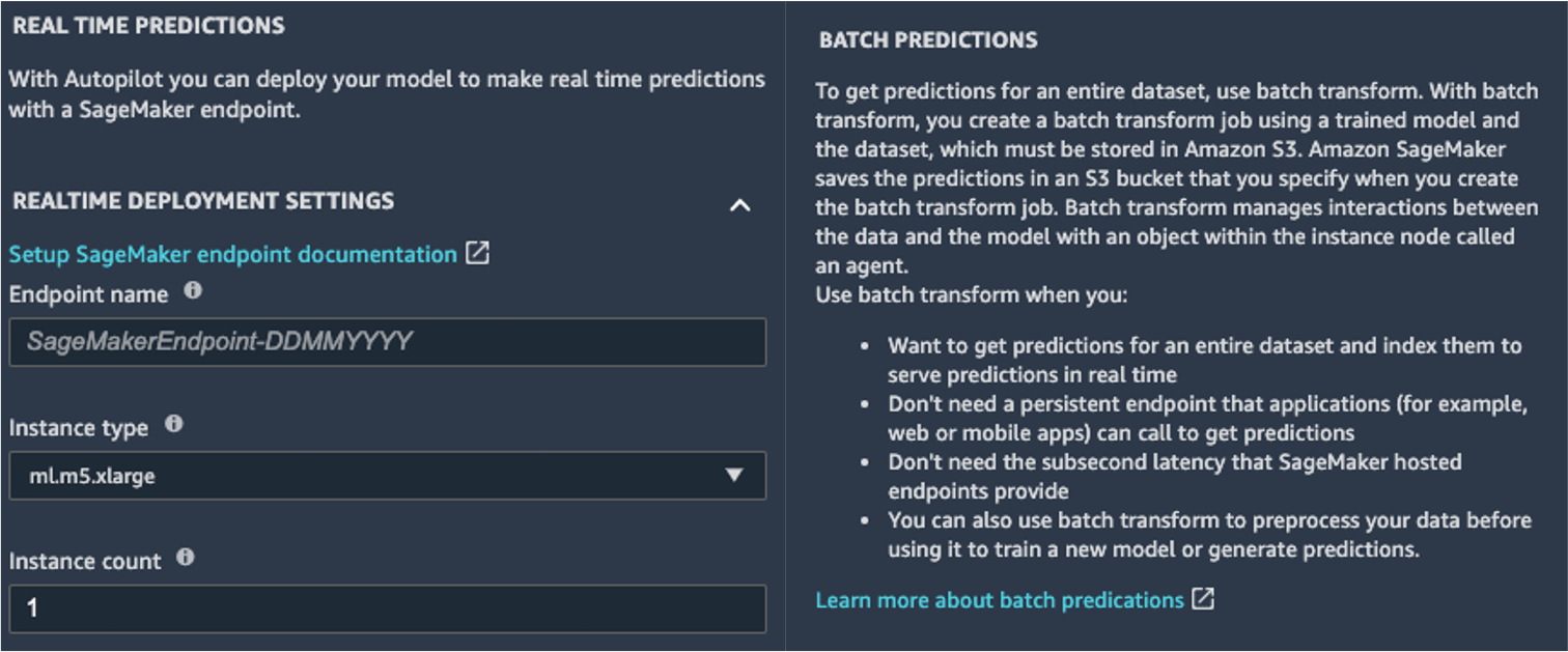
SageMaker shows you two options for deployment: a real-time endpoint, powered by Amazon SageMaker endpoints, and batch inference, powered by Amazon SageMaker batch transform.

SageMaker also provides other modes of inference. To learn more, see Deploy Models for Inference.

To enable the real-time predictions mode, you simply give the endpoint a name, an instance type, and an instance count. Because this model doesn’t require heavy compute resources, you can use a CPU-based instance with an initial count of 1. You can learn more about the different kind of instances available and their specs on the Amazon SageMaker Pricing page (in the On-Demand Pricing section, choose the Real-Time Inference tab). If you don’t know which instance you should choose for your deployment, you can also ask SageMaker to find the best one for you according to your KPIs by using the SageMaker Inference Recommender. You can also provide additional optional parameters, regarding whether or not you want to capture request and response data to or from the endpoint. This can prove useful if you’re planning on monitoring your model. You can also choose which content you wish to provide as part of your response—whether it’s just the prediction or the prediction probability, the probability of all classes, and the target labels.

To run a batch scoring job getting predictions for an entire set of inputs at one time, you can launch the batch transform job from the AWS Management Console or via the SageMaker Python SDK. To learn more about batch transform, refer to Use Batch Transform and the example notebooks.

Define a training pipeline

ML models can very rarely, if ever, be considered static and unchanging, because they drift from the baseline they’ve been trained on. Real-world data evolves over time, and more patterns and insights emerge from it, which may or may not be captured by the original model trained on historical data. To solve this problem, you can set up a training pipeline that automatically retrains your models with the latest data available.

In defining this pipeline, one of the options of the data scientist is to once again use AutoML for the training pipeline. You can launch an AutoML job programmatically by invoking the create_auto_ml_job() API from the AWS Boto3 SDK. You can call this operation from an AWS Lambda function within an AWS Step Functions workflow, or from a LambdaStep in Amazon SageMaker Pipelines.

Alternatively, the data scientist can use the knowledge, artifacts, and hyper-parameters obtained from the AutoML job to define a complete training pipeline. You need the following resources:

• The algorithm that worked best for the use case – You already obtained this information from the summary of the Canvas-generated model. For this use case, it’s the XGBoost built-in algorithm. For instructions on how to use the SageMaker Python SDK to train the XGBoost algorithm with SageMaker, refer to Use XGBoost with the SageMaker Python SDK.
  

• The hyperparameters derived by the AutoML job – These are available in the Explainability section. You can use them as inputs when defining the training job with the SageMaker Python SDK.
  

• The feature engineering code provided in the Artifacts section – You can use this code both for preprocessing the data before training (for example, via Amazon SageMaker Processing), or before inference (for example, as part of a SageMaker inference pipeline).
  

You can combine these resources as part of a SageMaker pipeline. We omit the implementation details in this post—stay tuned for more content coming on this topic.

Conclusion

SageMaker Canvas lets you use ML to generate predictions without needing to write any code. A business analyst can autonomously start using it with local datasets, as well as data already stored on Amazon Simple Storage Service (Amazon S3), Amazon Redshift, or Snowflake. With just a few clicks, they can prepare and join their datasets, analyze estimated accuracy, verify which columns are impactful, train the best performing model, and generate new individual or batch predictions, all without any need for pulling in an expert data scientist. Then, as needed, they can share the model with a team of data scientists or MLOps engineers, who import the models into SageMaker Studio, and work alongside the analyst to deliver a production solution.

Business analysts can independently gain insights from their data without having a degree in ML, and without having to write a single line of code. Data scientists can now have additional time to work on more challenging projects that can better use their extensive knowledge of AI and ML.

We believe this new collaboration opens the door to building many more powerful ML solutions for your business. You now have analysts producing valuable business insights, while letting data scientists and ML engineers help refine, tune, and extend as needed.

Additional Resources

• To learn more about how SageMaker can further help business analysts, refer to Amazon SageMaker for Business Analysts.
• To find out more about how SageMaker allows data scientists develop, train, and deploy their ML models, check out Amazon SageMaker for Data Scientists.
• For more information about how SageMaker can aid MLOps engineers in streamlining the ML lifecycle using MLOps, refer to Amazon SageMaker for MLOps Engineers.

About the Authors

Davide Gallitelli is a Specialist Solutions Architect for AI/ML in the EMEA region. He is based in Brussels and works closely with customers throughout Benelux. He has been a developer since he was very young, starting to code at the age of 7. He started learning AI/ML at university, and has fallen in love with it since then.

Mark Roy is a Principal Machine Learning Architect for AWS, helping customers design and build AI/ML solutions. Mark’s work covers a wide range of ML use cases, with a primary interest in computer vision, deep learning, and scaling ML across the enterprise. He has helped companies in many industries, including insurance, financial services, media and entertainment, healthcare, utilities, and manufacturing. Mark holds six AWS certifications, including the ML Specialty Certification. Prior to joining AWS, Mark was an architect, developer, and technology leader for over 25 years, including 19 years in financial services.

Read More

Many software as a service (SaaS) providers across various industries are adding machine learning (ML) and artificial intelligence (AI) capabilities to their SaaS offerings to address use cases like personalized product recommendation, fraud detection, and accurate demand protection. Some SaaS providers want to build such ML and AI capabilities themselves and deploy them in a multi-tenant environment. However, others who have more advanced customers want to allow their customers to build ML models themselves and use them to augment the SaaS with additional capabilities or override the default implementation of certain functionality.

In this post, we discuss how to enhance your SaaS offering with a data science workbench powered by Amazon SageMaker Studio.

Let’s say an independent software vendor (ISV) named XYZ has a leading CRM SaaS offering that is used by millions of customers to analyze customer purchase behavior. A marketer from the company FOO (an XYZ customer) wants to find their buyers with propensity to churn so they can optimize the ROI of their customer retention programs by targeting such buyers. They previously used simple statistical analysis in the CRM to assess such customers. Now, they want to further improve the ROI by using ML techniques. XYZ can improve their CRM for their customers by using the solution explained in this post and enable FOO’s data science team to build models themselves on top of their data.

SaaS customers interested in this use case want to have access to a data science workbench as part of the SaaS, through which they can access their data residing inside the SaaS with ease, analyze it, extract trends, and build, train, and deploy custom ML models. They want secure integration between the data science workbench and the SaaS, access to a comprehensive and broad set of data science and ML capabilities, and the ability to import additional datasets and join that with data extracted from the SaaS to derive useful insights.

The following diagram illustrates the as-is architecture of XYZ’s CRM SaaS offering.

This architecture consists of the following elements:

• Front-end layer – This layer is hosted on Amazon Simple Storage Service (Amazon S3). Amazon CloudFront is used as global content delivery network, and Amazon Cognito is used for user authentication and authorization. This layer includes three web applications:
  • Landing and sign-up – The public-facing page that customers can find and use to sign up for the CRM solution. Signing up triggers the registration process, which involves creating a new tenant in the system for the customer.
  • CRM application – Used by customers to manage opportunities, manage their own customers, and more. It relies on Amazon Cognito for authenticating and authorizing users.
  • CRM admin – Used by the SaaS provider for managing and configuring tenants.
• Backend layer – This layer is implemented as two sets of microservices running on Amazon Elastic Kubernetes Service (Amazon EKS):
  • SaaS services – Includes registration, tenant management, and user management services. A more complete implementation would include additional services for billing and metering.
  • Application services – Includes customer management, opportunity management, and product catalog services. This set might contain additional services based on the business functionalities provided by the CRM solution.

The next sections of the post discuss how to build a new version of the CRM SaaS with an embedded data science workbench.

Overview of solution

We use Amazon SageMaker to address the requirements of our solution. SageMaker is the most complete end-to-end service for ML. It’s a managed service for data scientists and developers that helps remove the undifferentiated heavy lifting associated with ML, so that you can have more time, resources, and energy to focus on your business.

The features of SageMaker include SageMaker Studio—the first fully integrated development environment (IDE) for ML. It provides a single web-based visual interface where you can perform all ML development steps required to build, train, tune, debug, deploy, and monitor models. It gives data scientists all the tools they need to take ML models from experimentation to production without leaving the IDE.

SageMaker Studio is embedded inside the SaaS as the data science workbench—you can launch it by choosing a link inside the SaaS and get access to the various capabilities of SageMaker. You can use SageMaker Studio to process and analyze your own data stored in the SaaS and extract insights. You can also use SageMaker APIs to build and deploy an ML model, then integrate SaaS processes and workflows with the deployed ML model for more accurate data processing.

This post addresses several considerations required for a solution:

• Multi-tenancy approach and accounts setup – How to isolate tenants. This section also discusses a proposed accounts structure.
• Provisioning and automation – How to automate the provisioning of the data science workbench.
• Integration and identity management – The integration between the SaaS and SageMaker Studio, and the integration with the identity provider (IdP).
• Data management – Data extraction and how to make it available to the data science workbench.

We discuss these concepts in the context of the CRM SaaS solution explained at the beginning of the post. The following diagram provides a high-level view of the solution architecture.

As depicted in the preceding diagram, the key change in the architecture is the introduction of the following components:

• Data management service – Responsible for extracting the SaaS customer’s data from the SaaS data store and pushing it to the data science workbench.
• Data science workbench management service – Responsible for provisioning the data science workbench for SaaS customers and launching it within the SaaS.
• Data science workbench – Based on SageMaker Studio, and runs in a separate AWS account. It also includes an S3 bucket that stores the data extracted from the SaaS data store.

The benefits of this solution include the following:

• SaaS customers can perform the various data science and ML tasks by launching SageMaker Studio from the SaaS in a separate tab, and use that as the data science workbench, without having to reauthenticate themselves. They don’t have to build and manage a separate data science platform.
• SaaS customers can easily extract data residing in the SaaS data store and make it available to the embedded data science workbench without having to have data engineering skills. Also, it’s easier to integrate the ML model they built with the SaaS.
• SaaS customers can access the broadest and most complete set of ML capabilities provided by SageMaker.

Multi-tenancy approach and account setup

This section covers how to provision SageMaker Studio for different tenants or SaaS customers (tenant and SaaS customers are used interchangeably because they’re closely related—each SaaS customer has a tenant). The following diagram depicts a multi-account setup that supports provisioning a secured and isolated SageMaker environment for each tenant. The proposed structure is in alignment with AWS best practices for a multi-account setup. For more information, refer to Organizing Your AWS Environment Using Multiple Accounts.

We use AWS Control Tower to implement the proposed multi-account setup. AWS Control Tower provides a framework to set up and extend a well-architected, multi-account AWS environment based on security and compliance best practices. AWS Control Tower uses multiple other AWS services, including AWS Organizations, AWS Service Catalog, and AWS CloudFormation, to build out its account structure and apply guardrails. The guardrails can be AWS Organizations service control policies or AWS Config rules. Account Factory, a feature of AWS Control Tower that enables the standardization of new account provisioning with the proper baselines for centralized logging and auditing, is used to automate the provisioning of new accounts for customers’ SageMaker environments as part of the onboarding process. Refer to AWS Control Tower – Set up & Govern a Multi-Account AWS Environment for more details about AWS Control Tower and how it uses other AWS services under the hood to set up and govern a multi-account setup.

All the accounts hosting customers’ SageMaker environments are under a common organizational unit (OU) to allow for applying common guardrails and automation, including a baseline configuration that creates a SageMaker Studio domain, S3 bucket in which the datasets extracted from SaaS data store reside, cross-account AWS Identity and Access Management (IAM) roles that allows for accessing SageMaker components from within the SaaS, and more.

Tenant isolation

In the context of the SaaS, you can consider various tenant isolation strategies:

• Silo model – Each tenant is running a fully siloed stack of resources
• Pool model – The same infrastructure and resources are shared across tenants
• Bridge model – A solution that involves a mix of the silo and pool models

Refer to the SaaS Tenant Isolation Strategies whitepaper for more details about SaaS tenant isolation strategies.

The silo model is used for SageMaker—a separate or independent SageMaker Studio domain is provisioned for each customer in a separate account as their instance of the data science workbench. The silo model simplifies security setup and isolation. It also provides other benefits like simplifying the calculation of costs associated with the tenant’s consumption of the various SageMaker capabilities.

While the silo isolation strategy is used for the SageMaker environment, the pool model is used for other components (such as the data science workbench management service). Establishing isolation in the silo model, where each tenant operates in its own infrastructure (an AWS account in this case) is much simpler compared to the pool model, where infrastructure is shared. The whitepaper referenced earlier provides guidance on how to establish isolation with a pool model. In this post, we use the following approach:

• The user is redirected to the IdP (Amazon Cognito in this case) for authentication. The user enters their user name and password, and upon successful authentication, the IdP returns a token that contains the user information and the tenant identifier. The front end includes the returned token in the subsequent HTTP requests sent by the front end to the microservices.
• When the microservice receives a request, it extracts the tenant identifier from the token included in the HTTP request, and assumes an IAM role that corresponds to the tenant. The assumed IAM role permissions are limited to the resources specific to the tenant. Therefore, even if the developer of the microservice made a mistake in the code and tried to access resources that belong to another tenant, the assumed IAM role doesn’t allow that action to proceed.
• The IAM role that corresponds to a tenant is created as part of the tenant registration and onboarding.

Other approaches for establishing isolation with pool mode include dynamic generation of policies and roles that are assumed by the microservice at runtime. For more information, refer to the SaaS Tenant Isolation Strategies whitepaper. Another alternative is using ABAC IAM policies—refer to How to implement SaaS tenant isolation with ABAC and AWS IAM for more details.

Provisioning and automation

As depicted earlier, we use AWS Organizations, AWS Service Catalog, and AWS CloudFormation StackSets to implement the required multi-account setup. An important aspect of that is creating a new AWS account per customer to host the SageMaker environment, and how to fully automate this process.

The StackSet for provisioning SageMaker in a customer’s account is created on the management account—the target for the StackSet is the ML OU. When a new account is created under the ML OU, a stack based on the template associated with the StackSet defined in the management account is automatically created in the new account.

Provisioning a SageMaker environment for a tenant is a multi-step process that takes a few minutes to complete. Therefore, an Amazon DynamoDB table is created to store the status of the SageMaker environment provisioning.

The following diagram depicts the flow for provisioning the data science workbench.

The data science workbench management microservice orchestrates the various activities for provisioning the data science workbench for SaaS customers. It calls the AWS Service Catalog ProvisionProduct API to initiate AWS account creation.

As mentioned earlier, the StackSet attached to the ML OU triggers the creation of a SageMaker Studio domain and other resources in a customer account as soon as the account is created under an ML OU as a result of the calling AWS Service Catalog ProvisionProduct API. Another way to achieve that is using AWS Service Catalog—you can create a product for provisioning the SageMaker Studio environment and add it to a portfolio. Then the portfolio is shared with all AWS accounts under the ML OU. The data science workbench management microservice has to make an explicit call to the AWS Service Catalog API after the completion of the AWS account creation to trigger the SageMaker Studio environment creation. AWS Service Catalog is very useful if you need to support multiple data science workbench variants—the user selects from a list of variants, and the data science workbench management microservice maps the user selection to a product defined in AWS Service Catalog. Then it invokes the ProvisionProduct API with the corresponding product ID.

After AWS account creation, a CreateManagedAccount event is published by AWS Control Tower to Amazon EventBridge. A rule is configured in EventBridge to send CreateManagedAccount events to an Amazon Simple Queue Service (Amazon SQS) queue. The data science workbench management microservice polls the SQS queue, retrieves CreateManagedAccount events, and invokes the tenant management service to add the created AWS account number (part of the event message) to the tenant metadata.

The state of the data science workbench provisioning requests is stored in a DynamoDB table so the users can inquire about it at any point of time.

Integration and identity management

This section focuses on the integration between SaaS and SageMaker Studio (which covers launching SageMaker Studio from within the SaaS) and identity management. We use Amazon Cognito as the IdP in this solution, but if the SaaS is already integrated with another IdP that supports OAuth 2.0/OpenID Connect, you can continue using that because the same design applies.

SageMaker Studio supports authentication via AWS Single Sign-On (AWS SSO) and IAM. Given that the AWS organization in this case is managed by the SaaS provider, it’s likely that AWS SSO is connected to the SaaS provider IdP, not the SaaS customer IdP. Therefore, we use IAM to authenticate users accessing SageMaker Studio.

Authenticating users accessing SageMaker Studio using IAM entails creating a user profile for each user on the SageMaker domain and mapping their identity in Amazon Cognito to the created user profile. One simple way to achieve that is by using their user name in Amazon Cognito as their user profile name in the SageMaker Studio domain. SageMaker provides the CreateUserProfile API, which can be used to programmatically creates a user profile for the user the first time they attempt to launch SageMaker Studio.

With regards to launching SageMaker Studio from within the SaaS, SageMaker exposes the CreatePresignedDomainUrl API, which generates the presigned URL for SageMaker Studio. The generated presigned URL is passed to the UI to launch SageMaker Studio in another browser tab.

The following diagram depicts the architecture for establishing integration between the SaaS and SageMaker Studio.

The data science workbench management microservice handles the generation of the presigned URL that is used to launch SageMaker Studio that exists in the customer account. It calls the tenant management microservice to retrieve the AWS account number that corresponds to the tenant ID included in the request, assumes an IAM role in this account with the required permissions, and calls the SageMaker CreatePresignedDomainUrl API to generate the presigned URL.

If the user is launching SageMaker Studio for the first time, a user profile needs to be created for them first. This is achieved by calling the SageMaker CreateUserProfile API.

The users can use the data science workbench to perform data processing at scale, train an ML model and using it for batch inference, and create enriched datasets. They can also use it to build and train an ML model, host this ML model on SageMaker managed hosting, and invoke it from the SaaS to realize a use case like the one mentioned at the beginning of the post (replacing a simple statistical analysis capability that predicts customer churn with an advanced ML-based capability that the customer themselves build the model for). The following diagram depicts one approach to achieve this.

The SaaS customer data scientist launches the data science workbench (SageMaker Studio) and uses it to preprocess the extracted data using SageMaker Processing (alternatively, you can use SageMaker Data Wrangler). They decide which ML algorithm to use and initiate a SageMaker training job to train the model with the preprocessed data. Then, they do the necessary model evaluation in a SageMaker Studio notebook, and if they’re happy with the results, they use SageMaker managed hosting to deploy and host the produced ML model.

After the ML is deployed, the data scientist goes to the SaaS and provides the details of the SageMaker endpoint hosting the ML model. This triggers a call to the tenant management microservice to add the SageMaker endpoint details to the tenant information. Then, when a call is made to the customer management microservice, it calls the tenant management microservice to retrieve tenant information, including the AWS account number and the SageMaker endpoint details. It then assumes an IAM role in the customer account with the required permissions, calls the SageMaker endpoint to calculate customer churn probability, and includes the output in the response message.

The ML endpoint called by the customer management microservice is dynamic (retrieved from the tenant management service), but the interface is fixed, and it is pre-defined by the SaaS provider – this includes the format (e.g., application/json), the features that the SaaS sends to the ML model, their ordering, and the output as well. The SaaS customer is expected to build an ML model that aligns with the interface defined by the SaaS provider. The interface details, and a sample request/response, are going to be presented to the SaaS customer on the app page that will allow them to override the implementation with their own ML model. The SaaS microservice (customer management microservice in the diagram above) performs the required transformation and serialization to produce the features expected by the ML endpoint in the specified format, invokes the ML endpoint, performs the required deserialization and transformation, and then include the inference output in the response returned by the microservice.

It may happen that the SaaS customer wants to exclude features that are not relevant to their model, or add features on top of what the SaaS passed. This can be achieved leveraging Use Your Own Inference Code, where they have full control over inference code.

Data management

This section covers a proposed architecture for building the data management microservice, which is one of the approaches you can follow to allow SaaS customers to access the data residing in the SaaS data store. The data management microservice receives data extraction requests from data scientists, and runs these requests in a controlled way to avoid negatively impacting SaaS data store performance. The microservice is also responsible for controlling access to the SaaS data store (which data elements are included in the data extract), and data masking and anonymization, if required.

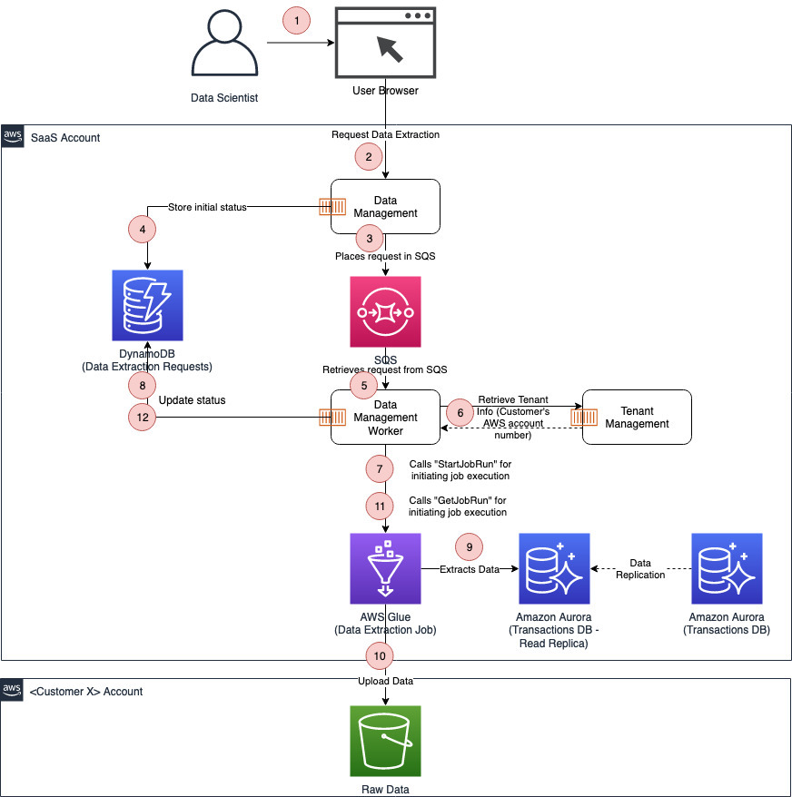
The following diagram depicts a potential design for the data management microservice.

The data management microservice is split into two components:

• Data management – Receives the data extraction request, places it in a queue, and sends an acknowledgment as a response
• Data management worker – Retrieves the request from the queue and processes it by calling an AWS Glue job

This decoupling allows you to scale the two components independently and control the load on the SaaS data store, regardless of the volume of the data extraction requests.

The AWS Glue job extracts the data from a replica for the transactions database, rather than the primary instance of the database. This prevents data extraction requests from negatively impacting the performance of the SaaS.

The AWS Glue job uploads the extracted data to an S3 bucket in the AWS account created a specific customer. Therefore, the data management worker component needs to call the tenant management microservice to retrieve the AWS account number, which is part of the tenant information.

The state of the data extraction requests is stored in a DynamoDB table so the users can inquire about it at any point of time.

Conclusion

In this post, we showed you how to build a data science workbench within your SaaS using SageMaker Studio. We have covered aspects like AWS account structure, tenant isolation, extracting data from the SaaS data store and making it accessible to the data science workbench, launching SageMaker Studio from within the SaaS, managing identities, and finally provisioning the data science workbench in an automated way using services like AWS Control Tower, AWS Organizations, and AWS CloudFormation.

We hope this helps you expand the usage of ML in your SaaS and provide your customers with a more flexible solution that allows them to consume the ML capabilities that you provide them and also to build ML capabilities themselves.

About the Authors

Islam Mahgoub is a Solutions Architect at AWS with 15 years of experience in application, integration, and technology architecture. At AWS, he helps customers build new cloud native solutions and modernise their legacy applications leveraging AWS services. Outside of work, Islam enjoys walking, watching movies, and listening to music.

Giuseppe Angelo Porcelli is a Principal Machine Learning Specialist Solutions Architect for Amazon Web Services. With several years software engineering an ML background, he works with customers of any size to deeply understand their business and technical needs and design AI and Machine Learning solutions that make the best use of the AWS Cloud and the Amazon Machine Learning stack. He has worked on projects in different domains, including MLOps, Computer Vision, NLP, and involving a broad set of AWS services. In his free time, Giuseppe enjoys playing football.

Arunprasath Shankar is an Artificial Intelligence and Machine Learning (AI/ML) Specialist Solutions Architect with AWS, helping global customers scale their AI solutions effectively and efficiently in the cloud. In his spare time, Arun enjoys watching sci-fi movies and listening to classical music.

Read More

Amazon SageMaker Autopilot is an automated machine learning (AutoML) solution that performs all the tasks you need to complete an end-to-end machine learning (ML) workflow. It explores and prepares your data, applies different algorithms to generate a model, and transparently provides model insights and explainability reports to help you interpret the results. Autopilot can also create a real-time endpoint for online inference. You can access Autopilot’s one-click features in Amazon SageMaker Studio or by using the AWS SDK for Python (Boto3) or the SageMaker Python SDK.

In this post, we show how to make batch predictions on an unlabeled dataset using an Autopilot-trained model. We use a synthetically generated dataset that is indicative of the types of features you typically see when predicting customer churn.

Solution overview

Batch inference, or offline inference, is the process of generating predictions on a batch of observations. Batch inference assumes you don’t need an immediate response to a model prediction request, as you would when using an online, real-time model endpoint. Offline predictions are suitable for larger datasets and in cases where you can afford to wait several minutes or hours for a response. In contrast, online inference generates ML predictions in real time, and is aptly referred to as real-time inference or dynamic inference. Typically, these predictions are generated on a single observation of data at runtime.

Losing customers is costly for any business. Identifying unhappy customers early on gives you a chance to offer them incentives to stay. Mobile operators have historical customer data showing those who have churned and those who have maintained service. We can use this historical information to construct a model to predict if a customer will churn using ML.

After we train an ML model, we can pass the profile information of an arbitrary customer (the same profile information that we used for training) to the model, and have the model predict whether or not the customer will churn. The dataset used for this post is hosted under the sagemaker-sample-files folder in an Amazon Simple Storage Service (Amazon S3) public bucket, which you can download. It consists of 5,000 records, where each record uses 21 attributes to describe the profile of a customer for an unknown US mobile operator. The attributes are as follows:

• State – US state in which the customer resides, indicated by a two-letter abbreviation; for example, TX or CA
• Account Length – Number of days that this account has been active
• Area Code – Three-digit area code of the corresponding customer’s phone number
• Phone – Remaining seven-digit phone number
• Int’l Plan – Has an international calling plan: Yes/No
• VMail Plan – Has a voice mail feature: Yes/No
• VMail Message – Average number of voice mail messages per month
• Day Mins – Total number of calling minutes used during the day
• Day Calls – Total number of calls placed during the day
• Day Charge – Billed cost of daytime calls
• Eve Mins, Eve Calls, Eve Charge – Billed cost for calls placed during the evening
• Night Mins, Night Calls, Night Charge – Billed cost for calls placed during nighttime
• Intl Mins, Intl Calls, Intl Charge – Billed cost for international calls
• CustServ Calls – Number of calls placed to Customer Service
• Churn? – Customer left the service: True/False

The last attribute, Churn?, is the target attribute that we want the ML model to predict. Because the target attribute is binary, our model performs binary prediction, also known as binary classification.

Prerequisites

Download the dataset to your local development environment and explore it by running the following S3 copy command with the AWS Command Line Interface (AWS CLI):

$ aws s3 cp s3://sagemaker-sample-files/datasets/tabular/synthetic/churn.txt ./

You can then copy the dataset to an S3 bucket within your own AWS account. This is the input location for Autopilot. You can copy the dataset to Amazon S3 by either manually uploading to your bucket or by running the following command using the AWS CLI:

$ aws s3 cp ./churn.txt s3://<YOUR S3 BUCKET>/datasets/tabular/datasets/churn.txt

Create an Autopilot experiment

When the dataset is ready, you can initialize an Autopilot experiment in SageMaker Studio. For full instructions, refer to Create an Amazon SageMaker Autopilot experiment.

Under Basic settings, you can easily create an Autopilot experiment by providing an experiment name, the data input and output locations, and specifying the target data to predict. Optionally, you can specify the type of ML problem that you want to solve. Otherwise, use the Auto setting, and Autopilot automatically determines the model based on the data you provide.

You can also run an Autopilot experiment with code using either the AWS SDK for Python (Boto3) or the SageMaker Python SDK. The following code snippet demonstrates how to initialize an Autopilot experiment using the SageMaker Python SDK. We use the AutoML class from the SageMaker Python SDK.

from sagemaker import AutoML

automl = AutoML(role="<SAGEMAKER EXECUTION ROLE>",
target_attribute_name="<NAME OF YOUR TARGET COLUMN>",
base_job_name="<NAME FOR YOUR AUTOPILOT EXPERIMENT>",
sagemaker_session="<SAGEMAKER SESSION>",
max_candidates="<MAX NUMBER OF TRAINING JOBS TO RUN AS PART OF THE EXPERIMENT>")

automl.fit("<PATH TO INPUT DATASET>", 
		   job_name="<NAME OF YOUR AUTOPILOT EXPERIMENT>", 
		   wait=False,
		   logs=False)

After Autopilot begins an experiment, the service automatically inspects the raw input data, applies feature processors, and picks the best set of algorithms. After it choose an algorithm, Autopilot optimizes its performance using a hyperparameter optimization search process. This is often referred to as training and tuning the model. This ultimately helps produce a model that can accurately make predictions on data it has never seen. Autopilot automatically tracks model performance, and then ranks the final models based on metrics that describe a model’s accuracy and precision.

You also have the option to deploy any of the ranked models either by choosing the model (right-click) and choosing Deploy model, or by selecting the model in the ranked list and choosing Deploy model.

Make batch predictions using a model from Autopilot

When your Autopilot experiment is complete, you can use the trained model to run batch predictions on your test or holdout dataset for evaluation. You can then compare the predicted labels against expected labels if your test or holdout dataset is pre-labeled. This is essentially a way to compare a model’s predictions to the truth. If more of the model’s predictions match the true labels, we can generally categorize the model as performing well. You can also run batch predictions to label unlabeled data. You can easily accomplish the same using the high-level SageMaker Python SDK with a few lines of code.

Describe a previously run Autopilot experiment

We first need to extract the information from a previously completed Autopilot experiment. We can use the AutoML class from the SageMaker Python SDK to create an automl object that encapsulates the information of a previous Autopilot experiment. You can use the experiment name you defined when initializing the Autopilot experiment. See the following code:

from sagemaker import AutoML

autopilot_experiment_name = "<ENTER YOUR AUTOPILOT EXPERIMENT NAME HERE>"
automl = AutoML.attach(auto_ml_job_name=autopilot_experiment_name)

With the automl object, we can easily describe and recreate the best trained model, as shown in the following snippets:

best_candidate = automl.describe_auto_ml_job()['BestCandidate']
best_candidate_name = best_candidate['CandidateName']

model = automl.create_model(name=best_candidate_name, 
	                    candidate=best_candidate, 
	                    inference_response_keys=inference_response_keys)

In some cases, you might want to use a model other than the best model as ranked by Autopilot. To find such a candidate model, you can use the automl object and iterate through the list of all or the top N model candidates and choose the model you want to recreate. For this post, we use a simple Python For loop to iterate through a list of model candidates:

all_candidates = automl.list_candidates(sort_by='FinalObjectiveMetricValue', 
                                         sort_order='Descending', 
			                 max_results=100)

for candidate in all_candidates:
	if candidate['CandidateName'] == "<ANY CANDIDATE MODEL OTHER THAN BEST MODEL>":
		candidate_name = candidate['CandidateName']
		model = automl.create_model(name=candidate_name, 
				                 candidate=candidate, 
				                 inference_response_keys=inference_response_keys)
		break

Customize the inference response

When recreating either the best or any other of Autopilot’s trained models, we can customize the inference response for the model by adding in the extra parameter inference_response_keys, as shown in the preceding example. You can use this parameter for both binary or multiclass classification problem types:

• predicted_label – The predicted class.
• probability – In binary classification, the probability that the result is predicted as the second or True class in the target column. In multiclass classification, the probability of the winning class.
• labels – A list of all possible classes.
• probabilities – A list of all probabilities for all classes (order corresponds with labels).

Because the problem we’re tackling in this post is binary classification, we set this parameter as follows in the preceding snippets while creating the models:

inference_response_keys = ['predicted_label', 'probability']

Create transformer and run batch predictions

Finally, after we recreate the candidate models, we can create a transformer to start the batch predictions job, as shown in the following two code snippets. While creating the transformer, we define the specifications of the cluster to run the batch job, such as instance count and type. The batch input and output are the Amazon S3 locations where our data inputs and outputs are stored. The batch prediction job is powered by SageMaker batch transform.

transformer = model.transformer(instance_count=1, 
				 instance_type='ml.m5.xlarge',
				 assemble_with='Line',
				 output_path=batch_output)
				 
transformer.transform(data=batch_input,
                      split_type='Line',
		      content_type='text/csv',
		      wait=False)

When the job is complete, we can read the batch output and perform evaluations and other downstream actions.

Summary

In this post, we demonstrated how to quickly and easily make batch predictions using Autopilot-trained models for your post-training evaluations. We used SageMaker Studio to initialize an Autopilot experiment to create a model for predicting customer churn. Then we referenced Autopilot’s best model to run batch predictions using the automl class with the SageMaker Python SDK. We also used the SDK to perform batch predictions with other model candidates. With Autopilot, we automatically explored and preprocessed our data, then created several ML models with one click, letting SageMaker take care of managing the infrastructure needed to train and tune our models. Lastly, we used batch transform to make predictions with our model using minimal code.

For more information on Autopilot and its advanced functionalities, refer to Automate model development with Amazon SageMaker Autopilot. For a detailed walkthrough of the example in the post, take a look at the following example notebook.

About the Authors

Arunprasath Shankar is an Artificial Intelligence and Machine Learning (AI/ML) Specialist Solutions Architect with AWS, helping global customers scale their AI solutions effectively and efficiently in the cloud. In his spare time, Arun enjoys watching sci-fi movies and listening to classical music.

Peter Chung is a Solutions Architect for AWS, and is passionate about helping customers uncover insights from their data. He has been building solutions to help organizations make data-driven decisions in both the public and private sectors. He holds all AWS certifications as well as two GCP certifications. He enjoys coffee, cooking, staying active, and spending time with his family.

Read More

In this post, we present a solution for digitizing transactional documents using Amazon Textract and incorporate a human review using Amazon Augmented AI (A2I). You can find the solution source at our GitHub repository.

Organizations must frequently process scanned transactional documents with structured text so they can perform operations such as fraud detection or financial approvals. Some common examples of transactional documents that contain tabular data include bank statements, invoices, and bills of materials. Manually extracting data from such documents is expensive, time-consuming, and often requires a significant investment in training a specialized workforce. With the architecture outlined in this post, you can digitize tabular data from even low-quality scanned documents and achieve a high degree of accuracy.

Significant strides have been made with machine learning (ML)-based algorithms to increase accuracy and reliability when processing scanned text documents. These algorithms often match human-level performance in recognizing text and extracting content. Amazon Textract is a fully managed service that automatically extracts printed text, handwriting, and other data from scanned documents. Additionally, Amazon Textract can automatically identify and extract forms and tables from scanned documents.

Companies dealing with complex, varying, and sensitive documents often need human oversight to ensure accuracy, consistency, and compliance of the extracted data. As human reviewers provide input, you can fine-tune AI models to capture subtle nuances of a particular business process. Amazon A2I is an ML service that makes it easy to build the workflows required for human review. Amazon A2I removes the undifferentiated heavy lifting associated with building human review systems or managing a large number of human reviewers, and provides a unified and secure experience to your workforce.

Extracting transactional data from scanned documents, such as a list of debit card transactions on a bank statement, poses a unique set of challenges. Combining artificial intelligence with human review provides a practical approach to overcome these hurdles. An integrated solution that combines Amazon Textract and Amazon A2I is one such compelling example.

Consumers routinely use their smartphones to scan and upload transactional documents. Depending on the overall scan quality, including lighting conditions, skewed perspective, and less-than-adequate image resolution, it’s not uncommon to see suboptimal accuracy when these documents are processed using computer vision (CV) techniques. At the same time, handling scanned documents using manual labor can result in increased processing costs and processing time, and can limit your ability to scale up the volume of documents a pipeline can handle.

Solution overview

The following diagram illustrates the workflow of our solution:

Our end-to-end workflow performs the following steps:

1. Extracts tables from scanned source documents.
2. Applies custom business rules when extracting data from the tables.
3. Selectively escalates challenging documents for human review.
4. Performs postprocessing on the extracted data.
5. Stores the results.

A custom user interface built with ReactJS is provided to human reviewers to intuitively and efficiently review and correct issues in the documents when Amazon Textract provides a low-confidence extraction score, for example when text is obscured, fuzzy, or otherwise unclear.

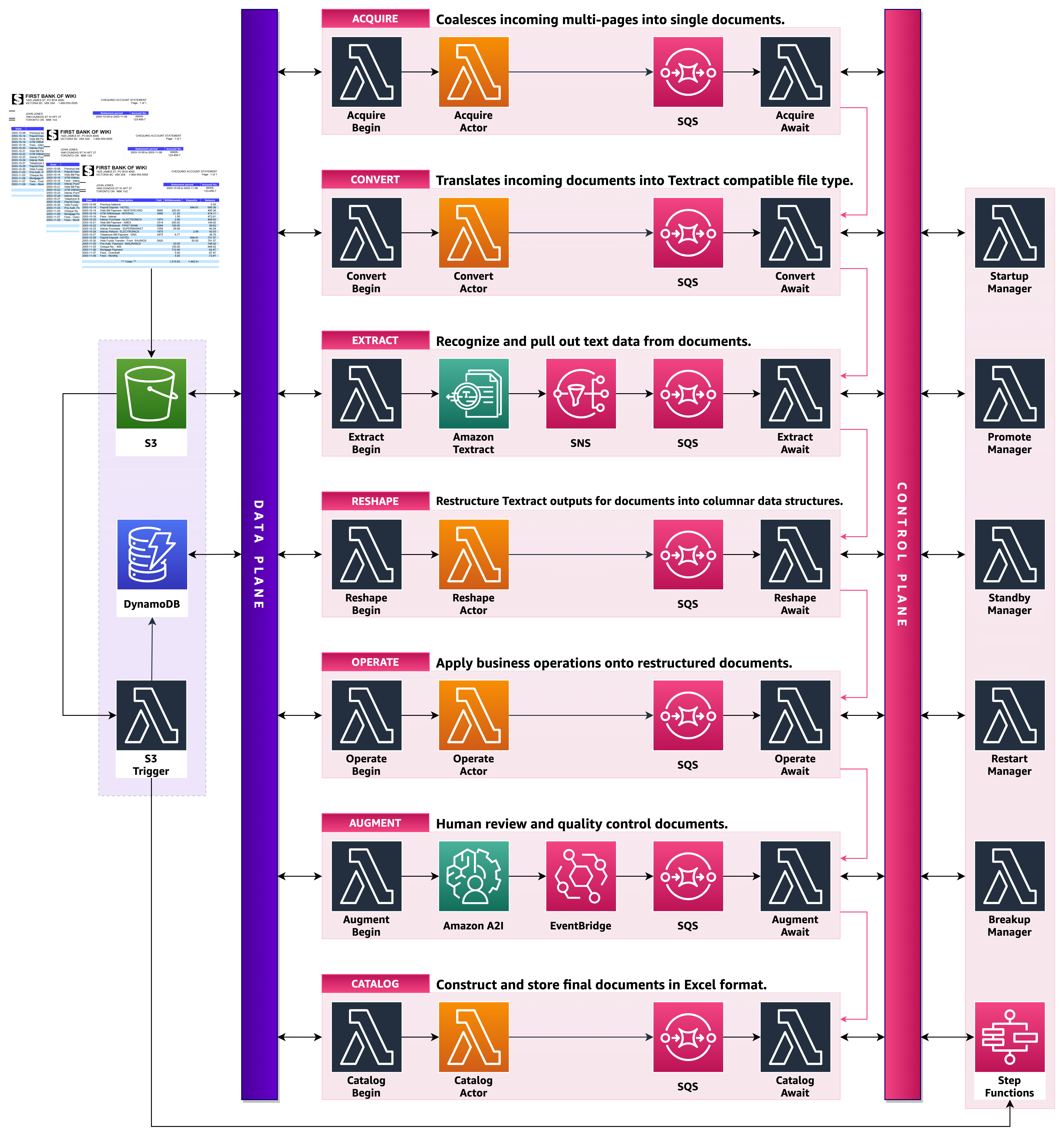
Our reference solution uses a highly resilient pipeline, as detailed in the following diagram, to coordinate the various document processing stages.

The solution incorporates several architectural best practices:

• Batch processing – When possible, the solution should collect multiple documents and perform batch operations so we can optimize throughput and use resources more efficiently. For example, calling a custom AI model to run inference one time for a group of documents, as opposed to calling the model for each document individually. The design of our solution should enable batching when appropriate.
• Priority adjustment – When the volume of documents in the queue increases and the solution is no longer able to process them in a timely manner, we need a way to indicate that certain documents are higher priority, and therefore must be processed ahead of other documents in the queue.
• Auto scaling – The solution should be capable of scaling up and down dynamically. Many document processing workflows need to support the cyclical nature of demand. We should design the solution such that it can seamlessly scale up to handle spikes in load and scale back down when the load subsides.
• Self-regulation – The solution should be capable of gracefully handling external service outages and rate limitations.

Document processing stages

In this section, we walk you through the details of each stage in the document processing workflow:

• Acquisition
• Conversion
• Extraction
• Reshaping
• Custom business operations
• Augmentation
• Cataloging

Acquisition

The first stage of the pipeline acquires input documents from Amazon Simple Storage Service (Amazon S3). In this stage, we store initial document information in an Amazon DynamoDB table after receiving an S3 event notification via Amazon Simple Queue Service (Amazon SQS). We use this table record to track the progression of this document across the entire pipeline.

The order of priority for each document is determined by sorting the alphanumeric input key prefix in the document path. For example, a document stored with key acquire/p0/doc.pdf results in priority p0, and takes precedence over another document stored with key acquire/p1/doc.pdf (resulting in priority p1). Documents with no priority indicator in the key are processed at the end.

Conversion

Documents acquired from the previous stage are converted into PDF format, so we can provide a consistent data format for the rest of the pipeline. This allows us to batch multiple pages of a related document.

Extraction

PDF documents are sent to Amazon Textract to perform optical character recognition (OCR). Results from Amazon Textract are stored as JSON in a folder in Amazon S3.

Reshaping

Amazon Textract provides detailed information from the processed document, including raw text, key-value pairs, and tables. A significant amount of additional metadata identifies the location and relationship between the detected entity blocks. The transactional data is selected for further processing at this stage.

Custom business operations

Custom business rules are applied to the reshaped output containing information about tables in the document. Custom rules may include table format detection (such as detecting that a table contains checking transactions) or column validation (such as verifying that a product code column only contains valid codes).

Augmentation

Human annotators use Amazon A2I to review the document and augment it with any information that was missed. The review includes analyzing each table in the document for errors such as incorrect table types, field headers, and individual cell text that was incorrectly predicted. Confidence scores provided by the extraction stage are displayed in the UI to help human reviewers locate less accurate predictions easily. The following screenshot shows the custom UI used for this purpose.

Our solution uses a private human review workforce consisting of in-house annotators. This is an ideal option when dealing with sensitive documents or documents that require highly specialized domain knowledge. Amazon A2I also supports human review workforces through Amazon Mechanical Turk and Amazon’s authorized data labeling partners.

Cataloging

Documents that pass human review are cataloged into an Excel workbook so your business teams can easily consume them. The workbook contains each table detected and processed in the source document in their respective sheet, which is labeled with table type and page number. These Excel files are stored in a folder in Amazon S3 for consumption by business applications, for example, performing fraud detection using ML techniques.

Deploy the solution

This reference solution is available on GitHub, and you can deploy it with the AWS Cloud Development Kit (AWS CDK). The AWS CDK uses the familiarity and expressive power of programming languages for modeling your applications. It provides high-level components called constructs that preconfigure cloud resources with proven defaults, so you can build cloud applications with ease.

For instructions on deploying the cloud application, refer to the README file in the GitHub repo.

Solution demonstration

The following video walks you through a demonstration of the solution.

Conclusion

This post showed how you can build a custom digitization solution to process transactional documents with Amazon Textract and Amazon A2I. We automated and augmented input manifests, and enforced custom business rules. We also provided an intuitive user interface for human workforces to review data with low confidence scores, make necessary adjustments, and use feedback to improve the underlying ML models. The ability to use a custom frontend framework like ReactJS allows us to create modern web applications that serve our precise needs, especially when using public, private, or third-party data labeling workforces.

For more information about Amazon Textract and Amazon A2I, see Using Amazon Augmented AI to Add Human Review to Amazon Textract Output. For video presentations, sample Jupyter notebooks, or information about use cases like document processing, content moderation, sentiment analysis, text translation, and more, see Amazon Augmented AI Resources.

About the Team

The Amazon ML Solutions Lab pairs your organization with ML experts to help you identify and build ML solutions to address your organization’s highest return-on-investment ML opportunities. Through discovery workshops and ideation sessions, the ML Solutions Lab “works backward” from your business problems to deliver a roadmap of prioritized ML use cases with an implementation plan to address them. Our ML scientists design and develop advanced ML models in areas such as computer vision, speech processing, and natural language processing to solve customers’ problems, including solutions requiring human review.

About the Authors

Pri Nonis is a Deep Learning Architect at the Amazon ML Solutions Lab, where he works with customers across various verticals, and helps them accelerate their cloud migration journey, and to solve their ML problems using state-of-the-art solutions and technologies.

Dan Noble is a Software Development Engineer at Amazon where he helps build delightful user experiences. In his spare time, he enjoys reading, exercising, and having adventures with his family.

Jae Sung Jang is a Software Development Engineer. His passion lies with automating manual process using AI Solutions and Orchestration technologies to ensure business execution.

Jeremy Feltracco is a Software Development Engineer with the Amazon ML Solutions Lab at Amazon Web Services. He uses his background in computer vision, robotics, and machine learning to help AWS customers accelerate their AI adoption.

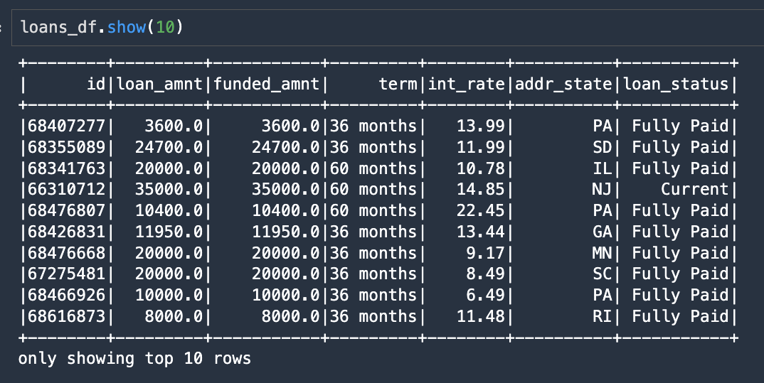
David Dasari is a manager at the Amazon ML Solutions Lab, where he helps AWS customers accelerate their AI and cloud adoption in the Human-In-The-Loop solutions across various industry verticals. With ERP and payment services as his background, was obsessed towards ML/AI taking strides in delighting customers that drove him to this field.

Read More

Data lakes have become the norm in the industry for storing critical business data. The primary rationale for a data lake is to land all types of data, from raw data to preprocessed and postprocessed data, and may include both structured and unstructured data formats. Having a centralized data store for all types of data allows modern big data applications to load, transform, and process whatever type of data is needed. Benefits include storing data as is without the need to first structure or transform it. Most importantly, data lakes allow controlled access to data from many different types of analytics and machine learning (ML) processes in order to guide better decision-making.

Multiple vendors have created data lake architectures, including AWS Lake Formation. In addition, open-source solutions allow companies to access, load, and share data easily. One of the options for storing data in the AWS Cloud is Delta Lake. The Delta Lake library enables reads and writes in open-source Apache Parquet file format, and provides capabilities like ACID transactions, scalable metadata handling, and unified streaming and batch data processing. Delta Lake offers a storage layer API that you can use to store data on top of an object-layer storage like Amazon Simple Storage Service (Amazon S3).

Data is at the heart of ML—training a traditional supervised model is impossible without access to high-quality historical data, which is commonly stored in a data lake. Amazon SageMaker is a fully managed service that provides a versatile workbench for building ML solutions and provides highly tailored tooling for data ingestion, data processing, model training, and model hosting. Apache Spark is a workhorse of modern data processing with an extensive API for loading and manipulating data. SageMaker has the ability to prepare data at petabyte scale using Spark to enable ML workflows that run in a highly distributed manner. This post highlights how you can take advantage of the capabilities offered by Delta Lake using Amazon SageMaker Studio.

Solution overview

In this post, we describe how to use SageMaker Studio notebooks to easily load and transform data stored in the Delta Lake format. We use a standard Jupyter notebook to run Apache Spark commands that read and write table data in CSV and Parquet format. The open-source library delta-spark allows you to directly access this data in its native format. This library allows you to take advantage of the many API operations to apply data transformations, make schema modifications, and use time-travel or as-of-timestamp queries to pull a particular version of the data.

In our sample notebook, we load raw data into a Spark DataFrame, create a Delta table, query it, display audit history, demonstrate schema evolution, and show various methods for updating the table data. We use the DataFrame API from the PySpark library to ingest and transform the dataset attributes. We use the delta-spark library to read and write data in Delta Lake format and to manipulate the underlying table structure, referred to as the schema.

We use SageMaker Studio, the built-in IDE from SageMaker, to create and run Python code from a Jupyter notebook. We have created a GitHub repository that contains this notebook and other resources to run this sample on your own. The notebook demonstrates exactly how to interact with data stored in Delta Lake format, which permits tables to be accessed in-place without the need to replicate data across disparate datastores.

For this example, we use a publicly available dataset from Lending Club that represents customer loans data. We downloaded the accepted data file (accepted_2007_to_2018Q4.csv.gz), and selected a subset of the original attributes. This dataset is available under the Creative Commons (CCO) License.

Prerequisites

You must install a few prerequisites prior to using the delta-spark functionality. To satisfy required dependencies, we have to install some libraries into our Studio environment, which runs as a Dockerized container and is accessed via a Jupyter Gateway app:

• OpenJDK for access to Java and associated libraries
• PySpark (Spark for Python) library
• Delta Spark open-source library

We can use either conda or pip to install these libraries, which are publicly available in either conda-forge, PyPI servers, or Maven repositories.

This notebook is designed to run within SageMaker Studio. After you launch the notebook within Studio, make sure you choose the Python 3(Data Science) kernel type. Additionally, we suggest using an instance type with at least 16 GB of RAM (like ml.g4dn.xlarge), which allows PySpark commands to run faster. Use the following commands to install the required dependencies, which make up the first several cells of the notebook:

%conda install openjdk -q -y
%pip install pyspark==3.2.0
%pip install delta-spark==1.1.0
%pip install -U "sagemaker>2.72"

After the installation commands are complete, we’re ready to run the core logic in the notebook.

Implement the solution

To run Apache Spark commands, we need to instantiate a SparkSession object. After we include the necessary import commands, we configure the SparkSession by setting some additional configuration parameters. The parameter with key spark.jars.packages passes the names of additional libraries used by Spark to run delta commands. The following initial lines of code assemble a list of packages, using traditional Maven coordinates (groupId:artifactId:version), to pass these additional packages to the SparkSession.

Additionally, the parameters with key spark.sql.extensions and spark.sql.catalog.spark_catalog enable Spark to properly handle Delta Lake functionality. The final configuration parameter with key fs.s3a.aws.credentials.provider adds the ContainerCredentialsProvider class, which allows Studio to look up the AWS Identity and Access Management (IAM) role permissions made available via the container environment. The code creates a SparkSession object that is properly initialized for the SageMaker Studio environment:

# Configure Spark to use additional library packages to satisfy dependencies

# Build list of packages entries using Maven coordinates (groupId:artifactId:version)
pkg_list = []
pkg_list.append("io.delta:delta-core_2.12:1.1.0")
pkg_list.append("org.apache.hadoop:hadoop-aws:3.2.2")

packages=(",".join(pkg_list))
print('packages: '+packages)

# Instantiate Spark via builder
# Note: we use the `ContainerCredentialsProvider` to give us access to underlying IAM role permissions

spark = (SparkSession
    .builder
    .appName("PySparkApp") 
    .config("spark.jars.packages", packages) 
    .config("spark.sql.extensions", "io.delta.sql.DeltaSparkSessionExtension") 
    .config("spark.sql.catalog.spark_catalog", "org.apache.spark.sql.delta.catalog.DeltaCatalog") 
    .config("fs.s3a.aws.credentials.provider", 
"com.amazonaws.auth.ContainerCredentialsProvider") 
    .getOrCreate()) 

sc = spark.sparkContext

print('Spark version: '+str(sc.version))

In the next section, we upload a file containing a subset of the Lending Club consumer loans dataset to our default S3 bucket. The original dataset is very large (over 600 MB), so we provide a single representative file (2.6 MB) for use by this notebook. PySpark uses the s3a protocol to enable additional Hadoop library functionality. Therefore, we modify each native S3 URI from the s3 protocol to use s3a in the cells throughout this notebook.

We use Spark to read in the raw data (with options for both CSV or Parquet files) with the following code, which returns a Spark DataFrame named loans_df:

loans_df = spark.read.csv(s3a_raw_csv, header=True)

The following screenshot shows the first 10 rows from the resulting DataFrame.

We can now write out this DataFrame as a Delta Lake table with a single line of code by specifying .format("delta") and providing the S3 URI location where we want to write the table data:

loans_df.write.format("delta").mode("overwrite").save(s3a_delta_table_uri)

The next few notebook cells show an option for querying the Delta Lake table. We can construct a standard SQL query, specify delta format and the table location, and submit this command using Spark SQL syntax:

sql_cmd = f'SELECT * FROM delta.`{s3a_delta_table_uri}` ORDER BY loan_amnt'
sql_results = spark.sql(sql_cmd)

The following screenshot shows the results of our SQL query as ordered by loan_amnt.

Interact with Delta Lake tables

In this section, we showcase the DeltaTable class from the delta-spark library. DeltaTable is the primary class for programmatically interacting with Delta Lake tables. This class includes several static methods for discovering information about a table. For example, the isDeltaTable method returns a Boolean value indicating whether the table is stored in delta format:

# Use static method to determine table type
print(DeltaTable.isDeltaTable(spark, s3a_delta_table_uri))

You can create DeltaTable instances using the path of the Delta table, which in our case is the S3 URI location. In the following code, we retrieve the complete history of table modifications:

deltaTable = DeltaTable.forPath(spark, s3a_delta_table_uri)
history_df = deltaTable.history()
history_df.head(3)

The output indicates the table has six modifications stored in the history, and shows the latest three versions.

Schema evolution

In this section, we demonstrate how Delta Lake schema evolution works. By default, delta-spark forces table writes to abide by the existing schema by enforcing constraints. However, by specifying certain options, we can safely modify the schema of the table.

First, let’s read data back in from the Delta table. Because this data was written out as delta format, we need to specify .format("delta") when reading the data, then we provide the S3 URI where the Delta table is located. Second, we write the DataFrame back out to a different S3 location where we demonstrate schema evolution. See the following code:

delta_df = (spark.read.format("delta").load(s3a_delta_table_uri))
delta_df.write.format("delta").mode("overwrite").save(s3a_delta_update_uri)

Now we use the Spark DataFrame API to add two new columns to our dataset. The column names are funding_type and excess_int_rate, and the column values are set to constants using the DataFrame withColumn method. See the following code:

funding_type_col = "funding_type"
excess_int_rate_col = "excess_int_rate"

delta_update_df = (delta_df.withColumn(funding_type_col, lit("NA"))
                           .withColumn(excess_int_rate_col, lit(0.0)))
delta_update_df.dtypes

A quick look at the data types (dtypes) shows the additional columns are part of the DataFrame.

Now we enable the schema modification, thereby changing the underlying schema of the Delta table, by setting the mergeSchema option to true in the following Spark write command:

(delta_update_df.write.format("delta")
 .mode("overwrite")
 .option("mergeSchema", "true") # option - evolve schema
 .save(s3a_delta_update_uri)
)

Let’s check the modification history of our new table, which shows that the table schema has been modified:

deltaTableUpdate = DeltaTable.forPath(spark, s3a_delta_update_uri)

# Let's retrieve history BEFORE schema modification
history_update_df = deltaTableUpdate.history()
history_update_df.show(3)

The history listing shows each revision to the metadata.

Conditional table updates

You can use the DeltaTable update method to run a predicate and then apply a transform whenever the condition evaluates to True. In our case, we write the value FullyFunded to the funding_type column whenever the loan_amnt equals the funded_amnt. This is a powerful mechanism for writing conditional updates to your table data.

deltaTableUpdate.update(condition = col("loan_amnt") == col("funded_amnt"),
    set = { funding_type_col: lit("FullyFunded") } )

The following screenshot shows our results.

In the final change to the table data, we show the syntax to pass a function to the update method, which in our case calculates the excess interest rate by subtracting 10.0% from the loan’s int_rate attribute. One more SQL command pulls records that meet our condition, using the WHERE clause to locate records with int_rate greater than 10.0%:

# Function that calculates rate overage (amount over 10.0)
def excess_int_rate(rate):
    return (rate-10.0)

deltaTableUpdate.update(condition = col("int_rate") > 10.0,
 set = { excess_int_rate_col: excess_int_rate(col("int_rate")) } )

The new excess_int_rate column now correctly contains the int_rate minus 10.0%.

Our last notebook cell retrieves the history from the Delta table again, this time showing the modifications after the schema modification has been performed:

# Finally, let's retrieve table history AFTER the schema modifications

history_update_df = deltaTableUpdate.history()
history_update_df.show(3)

The following screenshot shows our results.

Conclusion

You can use SageMaker Studio notebooks to interact directly with data stored in the open-source Delta Lake format. In this post, we provided sample code that reads and writes this data using the open source delta-spark library, which allows you to create, update, and manage the dataset as a Delta table. We also demonstrated the power of combining these critical technologies to extract value from preexisting data lakes, and showed how to use the capabilities of Delta Lake on SageMaker.

Our notebook sample provides an end-to-end recipe for installing prerequisites, instantiating Spark data structures, reading and writing DataFrames in Delta Lake format, and using functionalities like schema evolution. You can integrate these technologies to magnify their power to provide transformative business outcomes.

About the Authors

Paul Hargis has focused his efforts on Machine Learning at several companies, including AWS, Amazon, and Hortonworks. He enjoys building technology solutions and also teaching people how to make the most of it. Prior to his role at AWS, he was lead architect for Amazon Exports and Expansions helping amazon.com improve experience for international shoppers. Paul likes to help customers expand their machine learning initiatives to solve real-world problems.

Vedant Jain is a Sr. AI/ML Specialist Solutions Architect, helping customers derive value out of the Machine Learning ecosystem at AWS. Prior to joining AWS, Vedant has held ML/Data Science Specialty positions at various companies such as Databricks, Hortonworks (now Cloudera) & JP Morgan Chase. Outside of his work, Vedant is passionate about making music, using Science to lead a meaningful life & exploring delicious vegetarian cuisine from around the world.

Read More