Why Karrot Uses TFX, and How to Improve Productivity on ML Pipeline Development

Posted by Ukjae Jeong, Gyoung-yoon Yoo, and Myeonghyeon Song from Karrot

Karrot (the global service of Danggeun Market in Korea) is a local community service app that connects neighbors based on a secondhand marketplace. Danggeun Market was launched in 2015, and over 23 million people in Korea are using Danggeun Market in their local communities. Currently, Karrot is operated in 440 local communities in four countries: the U.K., the U.S., Canada, and Japan. In our service, scrolling through feeds to find inexpensive and useful items has become a daily pleasure for users. For better user experiences, we’ve been applying several machine learning models such as recommendation models.

We are also working on ways to effectively and efficiently apply ML models. In particular, we’re putting lots of effort into building machine learning pipelines for periodic deployment, rapid experiments, and continuous model improvement.

For the ML pipelines, we’ve been using TFX (TensorFlow Extended) for production. So in this article, we will briefly introduce why we use TFX, and how we utilize TFX to improve productivity.

Machine Learning in Karrot

There are many ML projects inside Karrot. ML models are running inside the services. For example, we use automation models to detect fraud, and there are recommendation models to improve the user experience on our app feed. If you are interested in detailed descriptions of the models, please refer to our team blogs, which are written in Korean.

As we’ve been using Kubeflow for our ML models, we were able to periodically train, experiment, and deploy models but still, we had some pain points. As we started to use TFX with Kubeflow last year, TFX pushed this line further and let the team easily use our production pipelines.

How TFX helps us with production ML

TFX helps build and deploy production ML pipelines easily with open and extendable design.

TFX, completely open-sourced in 2019, is an end-to-end platform for production ML pipelines. It supports writing ML workflows in component units, which then can be run in multiple environments – Apache Beam, Dataflow, Kubeflow, and Airflow. It also comes with well-written standard components for data ingestion/transformation, training, and deployment.

Standard Components

TFX provides several standard components. If you are looking for components for data ingestion, there are CsvExampleGen based on local CSV files, PrestoExampleGen, and BigQueryExampleGen which can ingest data directly from Presto, BigQuery, and many other sources with some customization. So you can easily process data from multiple sources just by connecting pre-built components to your TFX pipelines.

It can also handle large-scale data processing smoothly. Since the Transform component that performs feature engineering is implemented on Apache Beam, you can execute it on GCP Dataflow or another compute cluster in a distributed manner.

Of course, many other convenient components exist and are added constantly.

Component Reusability

In order to adapt TFX to our product, there is a need for custom components. TFX has a well-structured component design that enables us to create custom components naturally and easily connect them to existing TFX pipelines. A simple Python function or container can be transformed into a TFX component, or you can write the whole component in the exact same way as standard components are written. For more details, check out the custom component guide.

To enhance our productivity by delivering these advantages, we share custom components that have similar use cases among our ML pipelines as an internal library of Karrot Market.

Various Runners are Supported

TFX is compatible with a variety of environments. It can be run locally on your laptop or run on DataFlow, GCP’s batch data processing service compatible with Apache Beam. You can visualize the output by manually running each component in a Jupyter Notebook. TFX also supports KubeFlow and Vertex AI, which have recently been released with new features as well. Therefore, the pipeline code is written once, and can then be run almost anywhere. We can simply create development, experiment, and deployment environments at once. For that reason, the burden of deploying models to production was significantly reduced by using TFX for our services.

Technical lessons

As we set up our ML pipelines with TFX, code qualities and our experiences in model development have increased.

However, there were difficulties. We didn’t have a uniform project structure or best practices among our team. Maybe this is because TFX itself is relatively new and we’ve been using it before version 1. It became harder to understand codes and start to contribute. As the pipelines are becoming larger and more complex, it’s getting harder to understand the meaning of custom components, corresponding config values, and dependencies. In addition, it was difficult to introduce some of the latest features to the team.

Improving the Development Experience

We decided to create and use a template for TFX pipelines to make it easier to understand each other’s code, implement pipelines with the same pattern, and share know-how with each other. We merged components frequently used in Karrot and put them in a shared library so that ML pipelines can be developed very quickly.

It was expected that the template would accelerate the development of new projects. In addition, as mentioned above, we expected that each project would have a similar structure, making it easier to understand each other’s projects.

So far, we have briefly introduced the template project. Here are some of our considerations to make better use of TFX in this project.

Configuration first

We prioritize our configuration first. It should be enough to understand how pipelines work by reading their configuration. If we can understand specific settings very easily, we can set up various experiments and proceed with them to AB testing.

example_gen_config.proto written in Protocol Buffer(Protobuf), denotes the specification of config. config.pbtxt holds the values, and pipeline.py builds up the pipeline.

// config.pbtxt
example_gen_config {
big_query_example_gen_config {
query: "# query for example gen"
}


...
}

...
// example_gen_config.proto
message ExampleGenConfig {
oneof config {
BigQueryExampleGenConfig big_query_example_gen_config = 1;
CsvExampleGenConfig csv_example_gen_config = 2;
}

...
}

// When BigQueryExampleGen is used
message BigQueryExampleGenConfig {
optional string query = 1;
}

// When CsvExampleGenConfig is used
message CsvExampleGenConfig {
optional string input_base = 1;
}
# pipeline.py
def create_pipeline(config):
...
example_gen = _create_example_gen(config.example_gen_config)
...


def _create_example_gen(config: example_gen_config_pb2.ExampleGenConfig):
...

if config.HasField("big_query_example_gen_config"):
...
return ...


if config.HasField("csv_example_gen_config"):
...
return ...


raise ...

All configurations of ExampleGen are determined by a single ExampleGenConfig message. Similarly, all pipeline components only depend on their configs and are created from them. This way, you can understand the structure of the pipeline just by looking at the configuration file. There is also the intention to make customization and code understanding easier by separating the part that defines each component.

For example, let’s assume the following situation: In order to test the data transformation later, the Transform component needs to support various data processing methods. You might want to add a data augmentation process in the transform component. Then it should be done by adding a config related to the data augmentation function. Similarly, you can extend the predefined Protobuf specification to easily support multiple processing methods and make it easy to see which processing method to use.

Managing Configs with Protobuf

About the example code above, some people may wonder why they use Protobuf as a configuration tool. There are several reasons for this, and we will compare advantages with YAML, which is one of the common practices for configuration.

First, Protobuf has a robust interface, and validation such as type checking is convenient. There is no need to check whether any field is defined, as Protobuf defines the object structure in advance. In addition, it is useful to support backward/forward compatibility in a project under active development.

Also, you can easily check the pipeline structure. YAML has a hierarchical structure, but in the case of hydra, which is often used in the machine learning ecosystem, the stage (e.g. production, dev, alpha) settings are divided into several files, so we thought that Protobuf has better stability and visibility.

If you use Protobuf as your project setup tool, many of the Protobuf definitions defined in TFX can be reused.

TensorFlow Ecosystem with Bazel

Bazel is a language-independent build system that is easy to extend and supports a variety of languages and tools. From simple projects to large projects using multiple languages and tools, it can be used quickly and concisely in most situations. For more information, please refer to Bazel Vision on the Bazel documentation page.

Using Bazel in a Python project is an uncommon setting, but we used Bazel as the project build system of the TFX template project. A brief introduction to the reason is as follows.

First of all, it works really well with Protobuf. Because Bazel is a language-independent build system, you can easily tie your Protobuf build artifacts as dependencies with other builds without worry. In addition, the Protocol Buffer repository itself uses Bazel, so it is easy to integrate it into the Bazel-based project.

The second reason is the special environment of the TensorFlow ecosystem. Many projects in the TensorFlow ecosystem use Bazel, and TFX also uses Bazel, so you can easily link builds with other projects (TensorFlow, TFX) using Bazel.

Internal Custom TFX Modules

As mentioned before, we’ve been building an internal library for the custom TFX modules (especially the custom components) that are frequently used across multiple projects. Anyone in Karrot can add their components and share them with the team.

For example, we are using ArgoCD to manage applications(e.g. TF Serving) in Kubernetes clusters, so if someone develops a component for deploying with ArgoCD, we can easily share it via an internal library. The library now contains several custom modules for our team for productivity.

The reason why we can share our custom features as an internal shared library is probably thanks to the modular structure of TFX. Through this, we were able to improve the overall productivity of the team easily. We can reuse most of the components that were developed from several projects, and develop new projects very easily.

Conclusion

TFX provides lots of great features to develop production ML pipelines. We’re using TFX on Kubeflow for ML pipelines to develop, experiment, and deploy in a better way, and it brings us many benefits. So we decided to introduce how we are using TFX in this blog post.

To learn more about Karrot, check out our website (Korea, US, and Canada). For the TFX, check out the TFX documentation page.

Read More

Process larger and wider datasets with Amazon SageMaker Data Wrangler

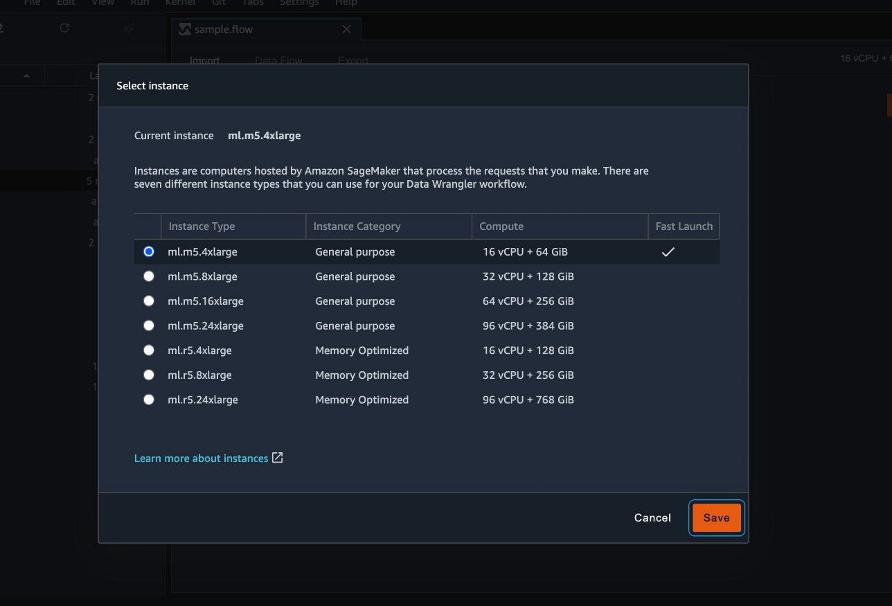
Amazon SageMaker Data Wrangler reduces the time to aggregate and prepare data for machine learning (ML) from weeks to minutes in Amazon SageMaker Studio. Data Wrangler can simplify your data preparation and feature engineering processes and help you with data selection, cleaning, exploration, and visualization. Data Wrangler has over 300 built-in transforms written in PySpark, so you can process datasets up to hundreds of gigabytes efficiently on the default instance, ml.m5.4xlarge.

However, when you work with datasets up to terabytes of data using built-in transforms, you might experience longer processing time or potential out-of-memory errors. Based on your data requirements, you can now use additional Amazon Elastic Compute Cloud (Amazon EC2) M5 instances and R5 instances. For example, you can start with a default instance (ml.m5.4xlarge) and then switch to ml.m5.24xlarge or ml.r5.24xlarge. You have the option of picking different instance types and finding the best trade-off of running cost and processing times. The next time you’re working on time series transformation and running heavy transformers to balance your data, you can right-size your Data Wrangler instance to run these processes faster.

When processing tens of gigabytes or even more with a custom Pandas transform, you might experience out-of-memory errors. You can switch from the default instance (ml.m5.4xlarge) to ml.m5.24xlarge, and the transform will finish without any errors. We thoroughly benchmarked and observed linear speedup as we increased instance size across a portfolio of datasets.

In this post, we share our findings from two benchmark tests to demonstrate how you can process larger and wider datasets with Data Wrangler.

Data Wrangler benchmark tests

Let’s review two tests we ran, aggregation queries and one-hot encoding, with different instance types using PySpark built-in transformers and custom Pandas transforms. Transformations that don’t require aggregation finish quickly and work well with the default instance type, so we focused on aggregation queries and transformations with aggregation. We stored our test dataset on Amazon Simple Storage Service (Amazon S3). This dataset’s expanded size is around 100 GB with 80 million rows and 300 columns. We used UI metrics to time benchmark tests and measure end-to-end customer-facing latency. When importing our test dataset, we disabled sampling. Sampling is enabled by default, and Data Wrangler only processes the first 100 rows when enabled.x

As we increased the Data Wrangler instance size, we observed a roughly linear speedup of Data Wrangler built-in transforms and custom Spark SQL. Pandas aggregation query tests only finished when we used instances larger than ml.m5.16xl, and Pandas needed 180 GB of memory to process aggregation queries for this dataset.

The following table summarizes the aggregation query test results.

Instance vCPU Memory (GiB) Data Wrangler built-in Spark transform time Pandas Time
(Custom Transform)
ml.m5.4xl 16 64 229 seconds Out of memory
ml.m5.8xl 32 128 130 seconds Out of memory
ml.m5.16xl 64 256 52 seconds 30 minutes

The following table summarizes the one-hot encoding test results.

Instance vCPU Memory (GiB) Data Wrangler built-in Spark transform time Pandas Time
(Custom Transform)
ml.m5.4xl 16 64 228 seconds Out of memory
ml.m5.8xl 32 128 130 seconds Out of memory
ml.m5.16xl 64 256 52 seconds Out of memory

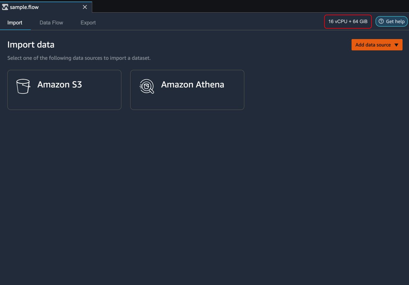
Switch the instance type of a data flow

To switch the instance type of your flow, complete the following steps:

  1. On the Amazon SageMaker Data Wrangler console, navigate to the data flow that you’re currently using.
  2. Choose the instance type on the navigation bar.
  3. Select the instance type that you want to use.
  4. Choose Save.

A progress message appears.

When the switch is complete, a success message appears.

Data Wrangler uses the selected instance type for data analysis and data transformations. The default instance and the instance you switched to (ml.m5.16xlarge) are both running. You can change the instance type or switch back to the default instance before running a specific transformation.

Shut down unused instances

You are charged for all running instances. To avoid incurring additional charges, shut down the instances that you aren’t using manually. To shut down an instance that is running, complete the following steps:

  1. On your data flow page, choose the instance icon in the left pane of the UI under Running instances.
  2. Choose Shut down.

If you shut down an instance used to run a flow, you can’t access the flow temporarily. If you get an error in opening the flow running an instance you previously shut down, wait for approximately 5 minutes and try opening it again.

Conclusion

In this post, we demonstrated how to process larger and wider datasets with Data Wrangler by switching instances to larger M5 or R5 instance types. M5 instances offer a balance of compute, memory, and networking resources. R5 instances are memory-optimized instances. Both M5 and R5 provide instance types to optimize cost and performance for your workloads.

To learn more about using data flows with Data Wrangler, refer to Create and Use a Data Wrangler Flow and Amazon SageMaker Pricing. To get started with Data Wrangler, see Prepare ML Data with Amazon SageMaker Data Wrangler.


About the Authors

Haider Naqvi is a Solutions Architect at AWS. He has extensive software development and enterprise architecture experience. He focuses on enabling customers to achieve business outcomes with AWS. He is based out of New York.

Huong Nguyen is a Sr. Product Manager at AWS. She is leading the data ecosystem integration for SageMaker, with 14 years of experience building customer-centric and data-driven products for both enterprise and consumer spaces.

Meenakshisundaram Thandavarayan is a Senior AI/ML specialist with AWS. He helps hi-tech strategic accounts on their AI and ML journey. He is very passionate about data-driven AI.

Sriharsha M Sr is an AI/ML Specialist Solutions Architect in the Strategic Specialist team at Amazon Web Services. He works with strategic AWS customers who are taking advantage of AI/ML to solve complex business problems. He provides technical guidance and design advice to implement AI/ML applications at scale. His expertise spans application architecture, big data, analytics, and machine learning.

Nikita Ivkin is an Applied Scientist, Amazon SageMaker Data Wrangler.

Read More

Fine-tune transformer language models for linguistic diversity with Hugging Face on Amazon SageMaker

Approximately 7,000 languages are in use today. Despite attempts in the late 19th century to invent constructed languages such as Volapük or Esperanto, there is no sign of unification. People still choose to create new languages (think about your favorite movie character who speaks Klingon, Dothraki, or Elvish).

Today, natural language processing (NLP) examples are dominated by the English language, the native language for only 5% of the human population and spoken only by 17%.

The digital divide is defined as the gap between those who can access digital technologies and those who can’t. Lack of access to knowledge or education due to language barriers also contributes to the digital divide, not only between people who don’t speak English, but also for the English-speaking people who don’t have access to non-English content, which reduces diversity of thought and knowledge. There is so much to learn mutually.

In this post, we summarize the challenges of low-resource languages and experiment with different solution approaches covering over 100 languages using Hugging Face transformers on Amazon SageMaker.

We fine-tune various pre-trained transformer-based language models for a question and answering task. We use Turkish in our example, but you could apply this approach to other supported language. Our focus is on BERT [1] variants, because a great feature of BERT is its unified architecture across different tasks.

We demonstrate several benefits of using Hugging Face transformers on Amazon SageMaker, such as training and experimentation at scale, and increased productivity and cost-efficiency.

Overview of NLP

There have been several major developments in NLP since 2017. The emergence of deep learning architectures such as transformers [2], the unsupervised learning techniques to train such models on extremely large datasets, and transfer learning have significantly improved the state-of-the-art in natural language understanding. The arrival of pre-trained model hubs has further democratized access to the collective knowledge of the NLP community, removing the need to start from scratch.

A language model is an NLP model that learns to predict the next word (or any masked word) in a sequence. The genuine beauty of language models as a starting point are three-fold: First, research has shown that language models trained on a large text corpus data learn more complex meanings of words than previous methods. For instance, to be able to predict the next word in a sentence, the language model has to be good at understanding the context, the semantics, and also the grammar. Second, to train a language model, labeled data—which is scarce and expensive—is not required during pre-training. This is important because an enormous amount of unlabeled text data is publicly available on the web in many languages. Third, it has been demonstrated that once the language model is smart enough to predict the next word for any given sentence, it’s relatively easy to perform other NLP tasks such as sentiment analysis or question answering with very little labeled data, because fine-tuning reuses representations from a pre-trained language model [3].

Fully managed NLP services have also accelerated the adoption of NLP. Amazon Comprehend is a fully managed service that enables text analytics to extract insights from the content of documents, and it supports a variety of languages. Amazon Comprehend supports custom classification and custom entity recognition and enables you to build custom NLP models that are specific to your requirements, without the need for any ML expertise.

Challenges and solutions for low-resource languages

The main challenge for a large number of languages is that they have relatively less data available for training. These are called low-resource languages. The m-BERT paper [4] and XLM-R paper [7] refer to Urdu and Swahili as low-resource languages.

The following figure specifies the ISO codes of over 80 languages, and the difference in size (in log-scale) between the two major pre-trainings [7]. In Wikipedia (orange), there are only 18 languages with over 1 million articles and 52 languages with over 1,000 articles, but 164 languages with only 1–10,000 articles [9]. The CommonCrawl corpus (blue) increases the amount of data for low-resource languages by two orders of magnitude. Nevertheless, they are still relatively small compared to high-resource languages such as English, Russian, or German.

In terms of Wikipedia article numbers, Turkish is another language in the same group of over 100,000 articles (28th), together with Urdu (54th). Compared with Urdu, Turkish would be regarded as a mid-resource language. Turkish has some interesting characteristics, which could make language models more powerful by creating certain challenges in linguistics and tokenization. It’s an agglutinative language. It has a very free word order, a complex morphology, or tenses without English equivalents. Phrases formed of several words in languages like English can be expressed with a single word form, as shown in the following example.

Turkish English
Kedi Cat
Kediler Cats
Kedigiller Family of cats
Kedigillerden Belonging to the family of cats
Kedileştirebileceklerimizdenmişçesineyken When it seems like that one is one those we can make cat

Two main solution approaches are language-specific models or multilingual models (with or without cross-language supervision):

  • Monolingual language models – The first approach is to apply a BERT variant to a specific target language. The more the training data, the better the model performance.
  • Multilingual masked language models – The other approach is to pre-train large transformer models on many languages. Multilingual language modeling aims to solve the lack of data challenge for low-resource languages by pre-training on a large number of languages so that NLP tasks learned from one language can be transferred to other languages. Multilingual masked language models (MLMs) have pushed the state-of-the-art on cross-lingual understanding tasks. Two examples are:

    • Multilingual BERT – The multilingual BERT model was trained in 104 different languages using the Wikipedia corpus. However, it has been shown that it only generalizes well across similar linguistic structures and typological features (for example, languages with similar word order). Its multilinguality is diminished especially for languages with different word orders (for example, subject/object/verb) [4].
    • XLM-R – Cross-lingual language models (XLMs) are trained with a cross-lingual objective using parallel datasets (the same text in two different languages) or without a cross-lingual objective using monolingual datasets [6]. Research shows that low-resource languages benefit from scaling to more languages. XLM-RoBERTa is a transformer-based model inspired by RoBERTa [5], and its starting point is the proposition that multilingual BERT and XLM are under-tuned. It’s trained on 100 languages using both the Wikipedia and CommonCrawl corpus, so the amount of training data for low-resource languages is approximately two orders of magnitude larger compared to m-BERT [7].

Another challenge of multilingual language models for low-resource languages is vocabulary size and tokenization. Because all languages use the same shared vocabulary in multilingual language models, there is a trade-off between increasing vocabulary size (which increases the compute requirements) vs. decreasing it (words not present in the vocabulary would be marked as unknown, or using characters instead of words as tokens would ignore any structure). The word-piece tokenization algorithm combines the benefits of both approaches. For instance, it effectively handles out-of-vocabulary words by splitting the word into subwords until it is present in the vocabulary or until the individual character is reached. Character-based tokenization isn’t very useful except for certain languages, such as Chinese. Techniques exist to address challenges for low-resource languages, such as sampling with certain distributions [6].

The following table depicts how three different tokenizers behave for the word “kedileri” (meaning “its cats”). For certain languages and NLP tasks, this would make a difference. For instance, for the question answering task, the model returns the span of the start token index and end token index; returning “kediler” (“cats”) or “kedileri” (“its cats”) would lose some context and lead to different evaluation results for certain metrics.

Pretrained Model Vocabulary size Tokenization for “Kedileri”*
dbmdz/bert-base-turkish-uncased 32,000 Tokens [CLS] kediler ##i [SEP]
Input IDs 2 23714 1023 3
bert-base-multilingual-uncased 105,879 Tokens [CLS] ked ##iler ##i [SEP]
Input IDs 101 30210 33719 10116 102
deepset/xlm-roberta-base-squad2 250,002 Tokens <s> ▁Ke di leri </s>
Input IDs 0 1345 428 1341 .
*In English: (Its) cats

Therefore, although low-resource languages benefit from multilingual language models, performing tokenization across a shared vocabulary may ignore some linguistic features for certain languages.

In the next section, we compare three approaches by fine-tuning them for a question answering task using a QA dataset for Turkish: BERTurk [8], multilingual BERT [4], and XLM-R [7].

Solution overview

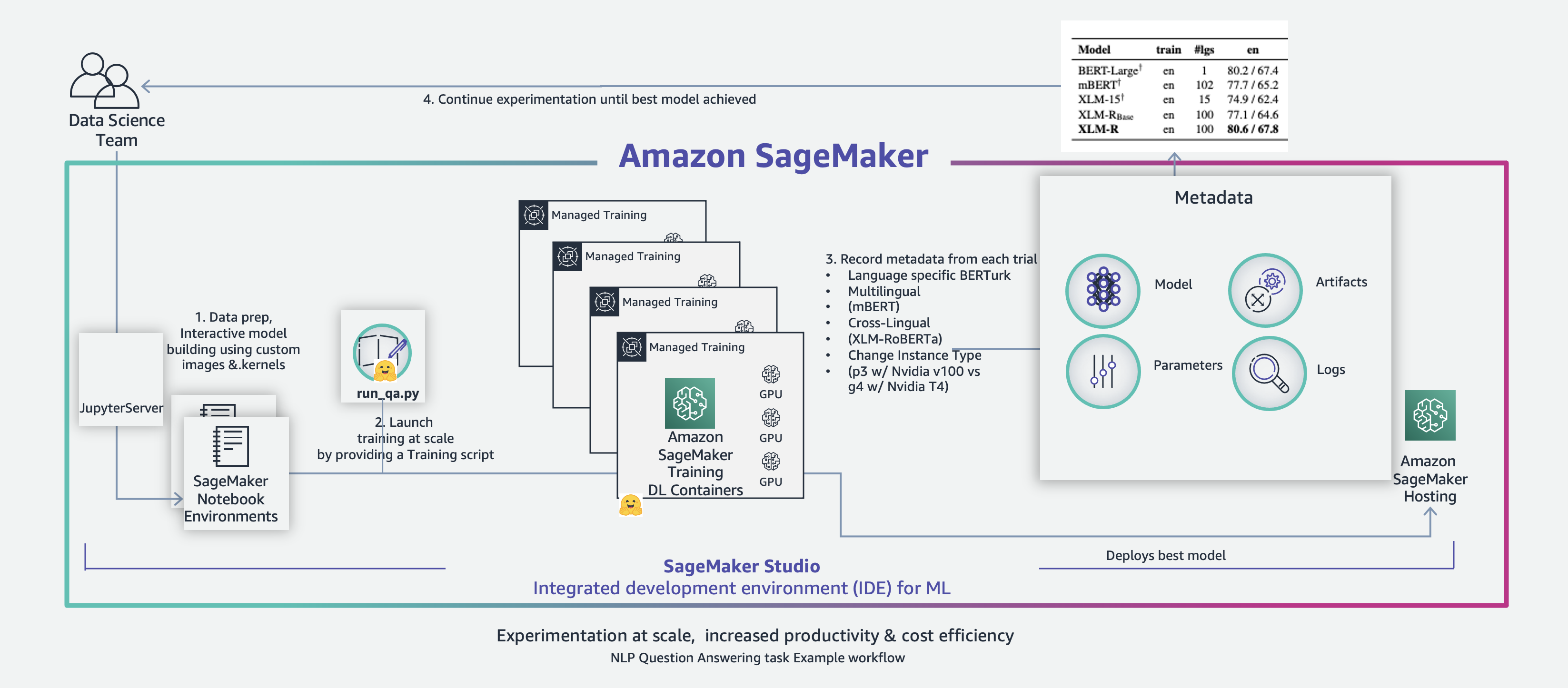
Our workflow is as follows:

  1. Prepare the dataset in an Amazon SageMaker Studio notebook environment and upload it to Amazon Simple Storage Service (Amazon S3).
  2. Launch parallel training jobs on SageMaker training deep learning containers by providing the fine-tuning script.
  3. Collect metadata from each experiment.
  4. Compare results and identify the most appropriate model.

The following diagram illustrates the solution architecture.

For more information on Studio notebooks, refer to Dive deep into Amazon SageMaker Studio Notebooks architecture. For more information on how Hugging Face is integrated with SageMaker, refer to AWS and Hugging Face collaborate to simplify and accelerate adoption of Natural Language Processing models.

Prepare the dataset

The Hugging Face Datasets library provides powerful data processing methods to quickly get a dataset ready for training in a deep learning model. The following code loads the Turkish QA dataset and explores what’s inside:

data_files = {}
data_files["train"] = 'data/train.json'
data_files["validation"] = 'data/val.json'

ds = load_dataset("json", data_files=data_files)

print("Number of features in dataset: n Train = {}, n Validation = {}".format(len(ds['train']), len(ds['validation'])))

There are about 9,000 samples.

The input dataset is slightly transformed into a format expected by the pre-trained models and contains the following columns:

df = pd.DataFrame(ds['train'])
df.sample(1)


The English translation of the output is as follows:

  • context – Resit Emre Kongar (b. 13 October 1941, Istanbul), Turkish sociologist, professor.
  • question – What is the academic title of Emre Kongar?
  • answer – Professor

Fine-tuning script

The Hugging Face Transformers library provides an example code to fine-tune a model for a question answering task, called run_qa.py. The following code initializes the trainer:

 # Initialize our Trainer
      trainer = QuestionAnsweringTrainer(
        model=model,
        args=training_args,
        train_dataset=train_dataset,
        eval_dataset=eval_dataset,
        eval_examples=eval_examples,
        tokenizer=tokenizer,
        data_collator=data_collator,
        post_process_function=post_processing_function,
        compute_metrics=compute_metrics,
    )

Let’s review the building blocks on a high level.

Tokenizer

The script loads a tokenizer using the AutoTokenizer class. The AutoTokenizer class takes care of returning the correct tokenizer that corresponds to the model:

tokenizer = AutoTokenizer.from_pretrained(
        model_args.model_name_or_path,
        cache_dir=model_args.cache_dir,
        use_fast=True,
        revision=model_args.model_revision,
        use_auth_token=None,
    )

The following is an example how the tokenizer works:

from transformers import AutoTokenizer

tokenizer = AutoTokenizer.from_pretrained("deepset/xlm-roberta-base-squad2")

input_ids = tokenizer.encode('İstanbulun en popüler hayvanı hangisidir? Kedileri', return_tensors="pt")
tokens = tokenizer('İstanbulun en popüler hayvanı hangisidir? Kedileri').tokens()

Model

The script loads a model. AutoModel classes (for example, AutoModelForQuestionAnswering) directly create a class with weights, configuration, and vocabulary of the relevant architecture given the name and path to the pre-trained model. Thanks to the abstraction by Hugging Face, you can easily switch to a different model using the same code, just by providing the model’s name. See the following example code:

    model = AutoModelForQuestionAnswering.from_pretrained(
        model_args.model_name_or_path,
        config=config,
        cache_dir=model_args.cache_dir,
        revision=model_args.model_revision,
    )

Preprocessing and training

The prepare_train_features() and prepare_validation_features() methods preprocess the training dataset and validation datasets, respectively. The code iterates over the input dataset and builds a sequence from the context and the current question, with the correct model-specific token type IDs (numerical representations of tokens) and attention masks. The sequence is then passed through the model. This outputs a range of scores, for both the start and end positions, as shown in the following table.

Input Dataset Fields Preprocessed Training Dataset Fields for QuestionAnsweringTrainer
id input_ids
title attention_mask
context start_positions
question end_positions
Answers { answer_start, answer_text } .

Evaluation

The compute_metrics() method takes care of calculating metrics. We use the following popular metrics for question answering tasks:

  • Exact match – Measures the percentage of predictions that match any one of the ground truth answers exactly.
  • F1 score – Measures the average overlap between the prediction and ground truth answer. The F1 score is the harmonic mean of precision and recall:

    • Precision – The ratio of the number of shared words to the total number of words in the prediction.
    • Recall – The ratio of the number of shared words to the total number of words in the ground truth.

Managed training on SageMaker

Setting up and managing custom machine learning (ML) environments can be time-consuming and cumbersome. With AWS Deep Learning Container (DLCs) for Hugging Face Transformers libraries, we have access to prepackaged and optimized deep learning frameworks, which makes it easy to run our script across multiple training jobs with minimal additional code.

We just need to use the Hugging Face Estimator available in the SageMaker Python SDK with the following inputs:

# Trial configuration
config['model'] = 'deepset/xlm-roberta-base-squad2'
config['instance_type'] = 'ml.p3.16xlarge'
config['instance_count'] = 2

# Define the distribution parameters in the HuggingFace Estimator

config['distribution'] = {'smdistributed':{'dataparallel':{ 'enabled': True }}}
trial_configs.append(config)

# We can specify a training script that is stored in a GitHub repository as the entry point for our Estimator, 
# so we don’t have to download the scripts locally.
git_config = {'repo': 'https://github.com/huggingface/transformers.git'}


    hyperparameters_qa={
        'model_name_or_path': config['model'],
        'train_file': '/opt/ml/input/data/train/train.json',
        'validation_file': '/opt/ml/input/data/val/val.json',
        'do_train': True,
        'do_eval': True,
        'fp16': True,
        'per_device_train_batch_size': 16,
        'per_device_eval_batch_size': 16,
        'num_train_epochs': 2,
        'max_seq_length': 384,
        'pad_to_max_length': True,
        'doc_stride': 128,
        'output_dir': '/opt/ml/model'
    }

    huggingface_estimator = HuggingFace(entry_point='run_qa.py',
                                        source_dir='./examples/pytorch/question-answering',
                                        git_config=git_config,
                                        instance_type=config['instance_type'],
                                        instance_count=config['instance_count'],
                                        role=role,
                                        transformers_version='4.12.3',
                                        pytorch_version='1.9.1',
                                        py_version='py38',
                                        distribution=config['distribution'],
                                        hyperparameters=hyperparameters_qa,
                                        metric_definitions=metric_definitions,
                                        enable_sagemaker_metrics=True,)
    
    nlp_training_job_name = f"NLPjob-{model}-{instance}-{int(time.time())}"
    
    training_input_path = f's3://{sagemaker_session_bucket}/{s3_prefix_qa}/'
    test_input_path = f's3://{sagemaker_session_bucket}/{s3_prefix_qa}/'
    
    huggingface_estimator.fit(
        inputs={'train': training_input_path, 'val': test_input_path},
        job_name=nlp_training_job_name,
        experiment_config={
            "ExperimentName": nlp_experiment.experiment_name,
            "TrialName": nlp_trial.trial_name,
            "TrialComponentDisplayName": nlp_trial.trial_name,},
        wait=False,
    )

Evaluate the results

When the fine-tuning jobs for the Turkish question answering task are complete, we compare the model performance of the three approaches:

  • Monolingual language model – The pre-trained model fine-tuned on the Turkish question answering text is called bert-base-turkish-uncased [8]. It achieves an F1 score of 75.63 and an exact match score of 56.17 in only two epochs and with 9,000 labeled items. However, this approach is not suitable for a low-resource language when a pre-trained language model doesn’t exist, or there is little data available for training from scratch.
  • Multilingual language model with multilingual BERT – The pre-trained model is called bert-base-multilingual-uncased. The multilingual BERT paper [4] has shown that it generalizes well across languages. Compared with the monolingual model, it performs worse (F1 score 71.73, exact match 50:45), but note that this model handles over 100 other languages, leaving less room for representing the Turkish language.
  • Multilingual language model with XLM-R – The pre-trained model is called xlm-roberta-base-squad2. The XLM-R paper shows that it is possible to have a single large model for over 100 languages without sacrificing per-language performance [7]. For the Turkish question answering task, it outperforms the multilingual BERT and monolingual BERT F1 scores by 5% and 2%, respectively (F1 score 77.14, exact match 56.39).

Our comparison doesn’t take into consideration other differences between models such as the model capacity, training datasets used, NLP tasks pre-trained on, vocabulary size, or tokenization.

Additional experiments

The provided notebook contains additional experiment examples.

SageMaker provides a wide range of training instance types. We fine-tuned the XLM-R model on p3.2xlarge (GPU: Nvidia V100 GPU, GPU architecture: Volta (2017)), p3.16xlarge (GPU: 8 Nvidia V100 GPUs), and g4dn.xlarge (GPU: Nvidia T4 GPU, GPU architecture: Turing (2018)), and observed the following:

  • Training duration – According to our experiment, the XLM-R model took approximately 24 minutes to train on p3.2xlarge and 30 minutes on g4dn.xlarge (about 23% longer). We also performed distributed fine-tuning on two p3.16xlarge instances, and the training time decreased to 10 minutes. For more information on distributed training of a transformer-based model on SageMaker, refer to Distributed fine-tuning of a BERT Large model for a Question-Answering Task using Hugging Face Transformers on Amazon SageMaker.
  • Training costs – We used the AWS Pricing API to fetch SageMaker on-demand prices to calculate it on the fly. According to our experiment, training cost approximately $1.58 on p3.2xlarge, and about four times less on g4dn.xlarge ($0.37). Distributed training on two p3.16xlarge instances using 16 GPUs cost $9.68.

To summarize, although the g4dn.xlarge was the least expensive machine, it also took about three times longer to train than the most powerful instance type we experimented with (two p3.16xlarge). Depending on your project priorities, you could choose from a wide variety of SageMaker training instance types.

Conclusion

In this post, we explored fine tuning pre-trained transformer-based language models for a question answering task for a mid-resource language (in this case, Turkish). You can apply this approach to over 100 other languages using a single model. As of writing, scaling up a model to cover all of the world’s 7,000 languages is still prohibitive, but the field of NLP provides an opportunity to widen our horizons.

Language is the principal method of human communication, and is a means of communicating values and sharing the beauty of a cultural heritage. The linguistic diversity strengthens intercultural dialogue and builds inclusive societies.

ML is a highly iterative process; over the course of a single project, data scientists train hundreds of different models, datasets, and parameters in search of maximum accuracy. SageMaker offers the most complete set of tools to harness the power of ML and deep learning. It lets you organize, track, compare, and evaluate ML experiments at scale.

Hugging Face is integrated with SageMaker to help data scientists develop, train, and tune state-of-the-art NLP models more quickly and easily. We demonstrated several benefits of using Hugging Face transformers on Amazon SageMaker, such as training and experimentation at scale, and increased productivity and cost-efficiency.

You can experiment with NLP tasks on your preferred language in SageMaker in all AWS Regions where SageMaker is available. The example notebook code is available in GitHub.

To learn how Amazon SageMaker Training Compiler can accelerate the training of deep learning models by up to 50%, see New – Introducing SageMaker Training Compiler.

The authors would like to express their deepest appreciation to Mariano Kamp and Emily Webber for reviewing drafts and providing advice.

References

  1. J. Devlin et al., “BERT: Pre-Training of Deep Bidirectional Transformers for Language Understanding”, (2018).
  2. A. Vaswani et al., “Attention Is All You Need”, (2017).
  3. J. Howard and S. Ruder, “Universal Language Model Fine-Tuning for Text Classification”, (2018).
  4. T. Pires et al., “How multilingual is Multilingual BERT?”, (2019).
  5. Y. Liu et al., “RoBERTa: A Robustly Optimized BERT Pretraining Approach”, (2019).
  6. G. Lample, and A. Conneau, “Cross-Lingual Language Model Pretraining”, (2019).
  7. A. Conneau et al., “Unsupervised Cross-Lingual Representation Learning at Scale”, (2019).
  8. Stefan Schweter. BERTurk – BERT models for Turkish (2020).
  9. Multilingual Wiki Statistics https://en.wikipedia.org/wiki/Wikipedia:Multilingual_statistics

About the Authors

Arnav Khare is a Principal Solutions Architect for Global Financial Services at AWS. His primary focus is helping Financial Services Institutions build and design Analytics and Machine Learning applications in the cloud. Arnav holds an MSc in Artificial Intelligence from Edinburgh University and has 18 years of industry experience ranging from small startups he founded to large enterprises like Nokia, and Bank of America. Outside of work, Arnav loves spending time with his two daughters, finding new independent coffee shops, reading and traveling. You can find me on LinkedIn and in Surrey, UK in real life.

Hasan-Basri AKIRMAK (BSc and MSc in Computer Engineering and Executive MBA in Graduate School of Business) is a Senior Solutions Architect at Amazon Web Services. He is a business technologist advising enterprise segment clients. His area of specialty is designing architectures and business cases on large scale data processing systems and Machine Learning solutions. Hasan has delivered Business development, Systems Integration, Program Management for clients in Europe, Middle East and Africa. Since 2016 he mentored hundreds of entrepreneurs at startup incubation programs pro-bono.

Heiko Hotz is a Senior Solutions Architect for AI & Machine Learning and leads the Natural Language Processing (NLP) community within AWS. Prior to this role, he was the Head of Data Science for Amazon’s EU Customer Service. Heiko helps our customers being successful in their AI/ML journey on AWS and has worked with organizations in many industries, including Insurance, Financial Services, Media and Entertainment, Healthcare, Utilities, and Manufacturing. In his spare time Heiko travels as much as possible.

Read More

Build a custom Q&A dataset using Amazon SageMaker Ground Truth to train a Hugging Face Q&A NLU model

In recent years, natural language understanding (NLU) has increasingly found business value, fueled by model improvements as well as the scalability and cost-efficiency of cloud-based infrastructure. Specifically, the Transformer deep learning architecture, often implemented in the form of BERT models, has been highly successful, but training, fine-tuning, and optimizing these models has proven to be a challenging problem. Thanks to the AWS and Hugging Face collaboration, it’s now simpler to train and optimize NLU models on Amazon SageMaker using the SageMaker Python SDK, but sourcing labeled data for these models is still difficult and time-consuming.

One NLU problem of particular business interest is the task of question answering. In this post, we demonstrate how to build a custom question answering dataset using Amazon SageMaker Ground Truth to train a Hugging Face question answering NLU model.

Question answering challenges

Question answering entails a model automatically producing an answer to a query given some body of text that may or may not contain the answer. For example, given the following question, “What workflows does SageMaker Ground Truth support?” a model should be able to identify the segment “annotation consolidation and audit” in the following paragraph:

SageMaker Ground Truth helps improve the quality of labels through annotation consolidation and audit workflows. Annotation consolidation is the process of collecting label inputs from two or more data labelers and combining them to create a single data label for your machine learning model. With built-in audit and review workflows, workers can perform label verification and make adjustments to improve accuracy.

This problem is challenging because it requires a model to comprehend the meaning of a question, rather than simply perform keyword search. Accurate models in this area can reduce customer support costs through powering intelligent chatbots, delivering high-quality voice assistant products, and driving online store revenue through personalized product question answering. One large dataset in this area is the Stanford Question Answering Dataset (SQuAD), a diverse question answering dataset that presents a model with short text passages and requires the model to predict the location of the answering text span in the passage. SQuAD is a reading comprehension dataset, consisting of questions posed by crowd workers on a set of Wikipedia articles, where the answer to every question is either a span of text from the corresponding passage, or otherwise marked impossible to answer.

One challenge in adapting SQuAD for business use cases is generating domain-specific custom datasets. This process of creating new question and answer datasets requires a specialized user interface that allows annotators to highlight spans and add questions to those spans. It must also be able to support the addition of impossible questions to support SQuAD 2.0 format, which includes non-answerable questions. These impossible questions help models gain additional understanding around which queries can’t be answered using the given passage. The custom worker templates in Ground Truth simplify the generation of these datasets by providing workers with a tailored annotation experience for creating question and answer datasets.

Solution overview

This solution creates and manages Ground Truth labeling jobs to label a domain-specific custom question-answer dataset using a custom annotation user interface. We use SageMaker to train, fine-tune, optimize, and deploy a Hugging Face BERT model built with PyTorch on a custom question answering dataset.

You can implement the solution by deploying the provided AWS CloudFormation template in your AWS account. AWS CloudFormation handles deploying the AWS Lambda functions that support pre-annotation and annotation consolidation for the annotation user interface. It also creates an Amazon Simple Storage Service (Amazon S3) bucket and the AWS Identity and Access Management (IAM) roles to use when creating a labeling job.

This post walks you through how to do the following:

  • Create your own question answering dataset, or augment an existing one using Ground Truth
  • Use Hugging Face datasets to combine and tokenize text
  • Fine-tune a BERT model on your question answering data using SageMaker training
  • Deploy your model to a SageMaker endpoint and visualize your results

Annotation user interface

We use a new custom worker task template with Ground Truth to add new annotations to the existing SQuAD dataset. This solution offers a worker task template as well as a pre-annotation Lambda function (which handles putting data into the user interface) and post-annotation Lambda function (which extracts results from the user interface after labeling is complete).

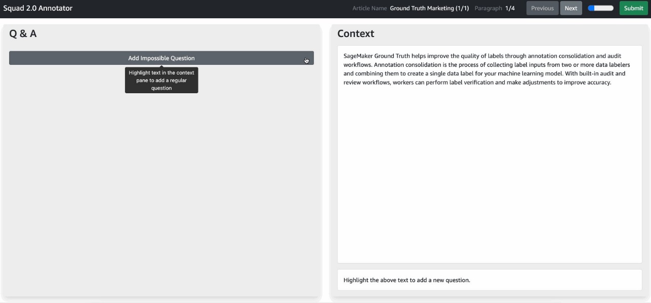
This custom worker task template gives you the ability to highlight text in the right pane, then add a corresponding question in the left pane that relates to the highlighted text. Highlighted text on the right pane can also be added to any previously created question. Moreover, you can add impossible questions according to SQuAD 2.0 format. Impossible questions allow models to reduce the number of unreliable false positive guesses when the passage is unable to answer a query.
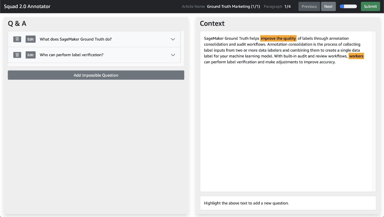
This user interface uses the same JSON schema as the SQuAD 2.0 dataset, which means it can operate over multiple articles and paragraphs, displaying one paragraph at a time using the Previous and Next buttons. The user interface makes it easy to monitor and determine the labeling work each annotator needs to complete during the task submission step.

Because the annotation UI is contained in a single Liquid HTML file, you can customize the labeling experience with knowledge of basic JavaScript. You can also modify Liquid tags to pass additional information into the labeling UI, and you can modify the template itself to include more detailed worker instructions.

Estimated costs

Deploying this solution can incur a maximum cost of around $20, not accounting for human labeling costs. Amazon S3, Lambda, SageMaker, and Ground Truth all offer the AWS Free Tier, with charges for additional usage. For more information, see the following pricing pages:

Prerequisites

To implement this solution, you should have the following prerequisites:

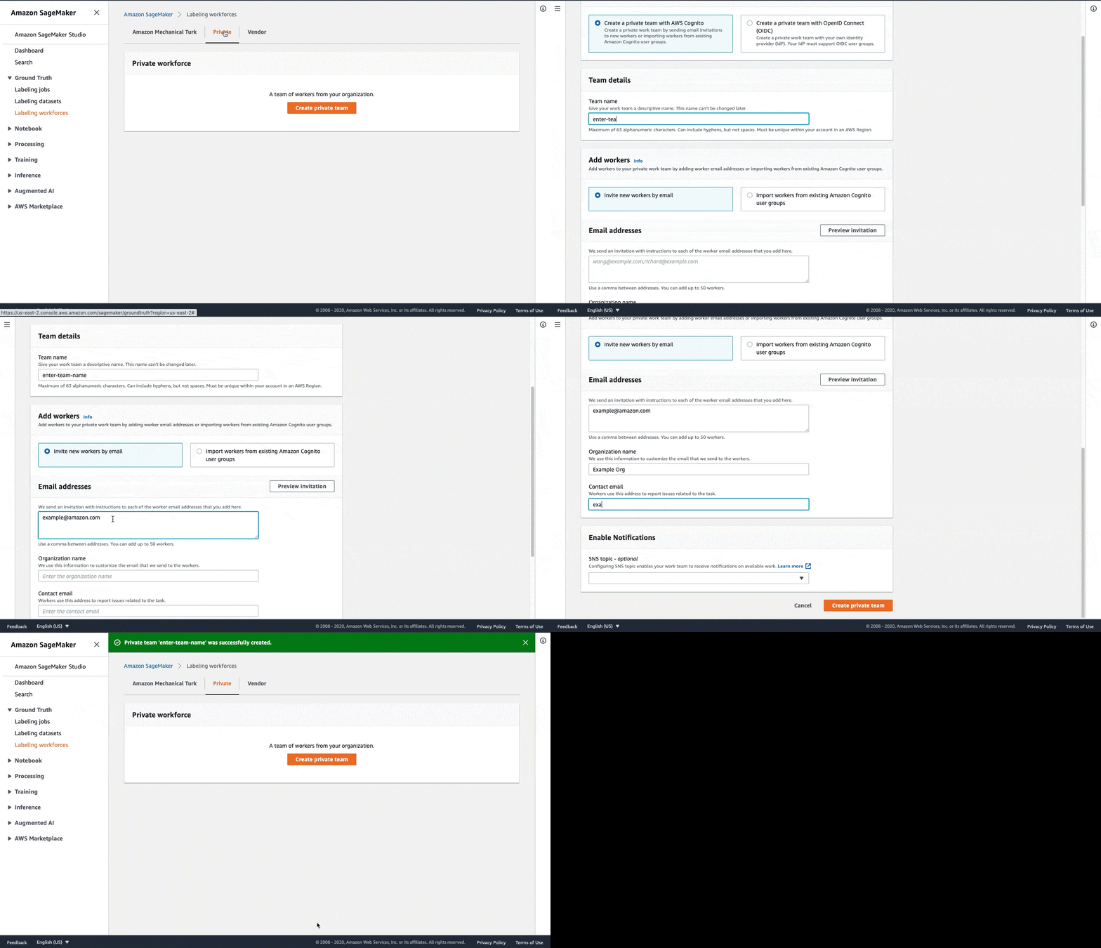
The following GIF demonstrates how to create a private workforce. For instructions, see Create an Amazon Cognito Workforce Using the Labeling Workforces Page.
Launch the CloudFormation Stack

Now that you’ve seen the structure of the solution, you deploy it into your account so you can run an example workflow. All the deployment steps related to the labeling pipeline are managed by AWS CloudFormation. This means AWS CloudFormation creates your pre-annotation and annotation consolidation Lambda functions, as well as an S3 bucket to store input and output data.

You can launch the stack in AWS Region us-east-1 on the AWS CloudFormation console using the Launch Stack button. To launch the stack in a different Region, use the instructions found in the README of the GitHub repository.

Operate the notebook

After the solution has been deployed to your account, a notebook instance named gt-hf-squad-notebook is available in your account. To start operating the notebook, complete the following steps:

  1. On the Amazon SageMaker console, navigate to the notebook instance page.
  2. Choose Open JupyterLab to open the instance.
  3. Inside the instance, browse to the repository hf-gt-custom-qa and open the notebook hf_squad_finetuning.ipynb.
  4. Choose conda_pytorch_p38 as your kernel.

Now that you’ve created a notebook instance and opened the notebook, you can run cells in the notebook to operate the solution. The remainder of this post provides additional details to each section in the notebook as you go along.

Download and inspect the data

The SQuAD dataset contains a training dataset as well as test and development datasets. The notebook downloads the SQuAD2.0 dataset for you, but you can choose which version of SQuAD to use by modifying the notebook cell under Download and inspect the data.

SQuAD was created by Pranav Rajpurkar, Jian Zhang, Konstantin Lopyrev, and Percy Liang. For more information, refer to the original paper and dataset. SQuAD has been licensed by the authors under the Creative Commons Attribution-ShareAlike 4.0 International Public License.

Let’s look at an example question and answer pair from SQuAD:

Paragraph title: Immune_system

The immune system is a system of many biological structures and processes within an organism that protects against disease. To function properly, an immune system must detect a wide variety of agents, known as pathogens, from viruses to parasitic worms, and distinguish them from the organism’s own healthy tissue. In many species, the immune system can be classified into subsystems, such as the innate immune system versus the adaptive immune system, or humoral immunity versus cell-mediated immunity. In humans, the blood–brain barrier, blood–cerebrospinal fluid barrier, and similar fluid–brain barriers separate the peripheral immune system from the neuroimmune system which protects the brain.

Question: The immune system protects organisms against what?

Answer: disease

Load model

Now that you’ve viewed an example question and answer pair in SQuAD, you can download a model that you can fine-tune for question answering. Hugging Face allows you to easily download a base model that has undergone large-scale pre-training and reinitialize it for a different downstream task. In this case, you download the distilbert-base-uncased model and repurpose it for question answering using the AutoModelForQuestionAnswering class from Hugging Face. You also utilize the AutoTokenizer class to retrieve the model’s pre-trained tokenizer. We dive deeper into the model we use later in the post.

View BERT input

BERT requires you to transform text data into a numeric representation known as tokens. There are a variety of tokenizers available; the following tokens were created by a tokenizer specifically designed for BERT that you instantiate with a set vocabulary. Each token maps to a word in the vocabulary. Let’s look at the transformed immune system question and context you supply BERT for inference.

{'input_ids': tensor([[    0,   133,  9161,   467, 15899, 28340,   136,    99,   116,     2,
             2,   133,  9161,   467,    16,    10,   467,     9,   171, 12243,
          6609,     8,  5588,   624,    41, 33993,    14, 15899,   136,  2199,
             4,   598,  5043,  5083,     6,    41,  9161,   467,   531, 10933,
            10,  1810,  3143,     9,  3525,     6,   684,    25, 35904,     6,
            31, 21717,     7, 43108, 31483,     6,     8, 22929,   106,    31,
             5, 33993,    18,   308,  2245, 11576,     4,    96,   171,  4707,
             6,     5,  9161,   467,    64,    28,  8967,    88, 44890,    29,
             6,   215,    25,     5, 36154,  9161,   467,  4411,     5, 28760,
          9161,   467,     6,    50, 10080, 15010, 17381,  4411,  3551,    12,
         43728, 17381,     4,    96,  5868,     6,     5,  1925,  2383, 36436,
          9639,     6,  1925,  2383,  1755,   241,  7450,  4182,  6204, 12293,
          9639,     6,     8,  1122, 12293,  2383, 36436,  7926,  2559,     5,
         27727,  9161,   467,    31,     5, 14913, 42866,   467,    61, 15899,
             5,  2900,     4,     2]]), 'attention_mask': tensor([[1, 1, 1, 1, 1, 1, 1, 1, 1, 1, 1, 1, 1, 1, 1, 1, 1, 1, 1, 1, 1, 1, 1, 1,
         1, 1, 1, 1, 1, 1, 1, 1, 1, 1, 1, 1, 1, 1, 1, 1, 1, 1, 1, 1, 1, 1, 1, 1,
         1, 1, 1, 1, 1, 1, 1, 1, 1, 1, 1, 1, 1, 1, 1, 1, 1, 1, 1, 1, 1, 1, 1, 1,
         1, 1, 1, 1, 1, 1, 1, 1, 1, 1, 1, 1, 1, 1, 1, 1, 1, 1, 1, 1, 1, 1, 1, 1,
         1, 1, 1, 1, 1, 1, 1, 1, 1, 1, 1, 1, 1, 1, 1, 1, 1, 1, 1, 1, 1, 1, 1, 1,
         1, 1, 1, 1, 1, 1, 1, 1, 1, 1, 1, 1, 1, 1, 1, 1, 1, 1, 1, 1, 1, 1, 1, 1]])}

Model inference

Now that you’ve seen what BERT takes as input, let’s look at how you can get inference results from the model. The following code demonstrates how to use the previously generated tokenized input and return inference results from the model. Similar to how BERT can’t accept raw text as input, it doesn’t generate raw text as output either. You translate BERT’s output by identifying the start and end points in the paragraph that BERT identified as the answer. Then you map that output to our tokens and back to English text.

outputs = model(**inputs, start_positions=start_positions, end_positions=end_positions)

answer_start_scores = outputs.start_logits
answer_end_scores = outputs.end_logits
answer_start = torch.argmax(
answer_start_scores
) # Get the most likely beginning of answer with the argmax of the score
answer_end = torch.argmax(answer_end_scores) + 1 # Get the most likely end of answer with the argmax of the score
answer = tokenizer.convert_tokens_to_string(tokenizer.convert_ids_to_tokens(input_ids[answer_start:answer_end]))
print(f"Question: {sq['paragraphs'][0]['qas'][0]['question']}")
print(f"Answer: {answer}")

The translated results are as follows:

Question: The immune system protects organisms against what?

Answer: disease

Augment SQuAD

Next, to obtain additional labeled data, we use a custom worker task template in Ground Truth. We can first create a new article in SQuAD format. The notebook copies this file from the repo to Amazon S3, but feel free to make any edits before running the Augment SQuAD cell. The format of SQuAD is shown in the following code. Each SQuAD JSON file contains multiple articles stored in the data key. Each article has a title field and one or more paragraphs. These paragraphs contain segments of text called context and any associated questions in the qas list. Because we’re annotating from scratch, we can leave the qas list empty and just provide context. The user interface is able to loop across both paragraphs and articles, allowing you to make each worker task as large or small as desired.

s3://<my-bucket-name>/custom_squad.json:

{
  "version": "v2.0",
  "data": [
    {
      "title": "Ground Truth Marketing",
      "paragraphs": [
        {
          "qas": [],
          "context": "SageMaker Ground Truth helps improve the quality of labels through annotation consolidation and audit workflows. Annotation consolidation is the process of collecting label inputs from two or more data labelers and combining them to create a single data label for your machine learning model. With built-in audit and review workflows, workers can perform label verification and make adjustments to improve accuracy."
        },
        {
          "qas": [],
          "context": "SageMaker Ground Truth provides automated labeling features such as ‘auto-segment’, ‘automatic 3D cuboid snapping’, and ‘sensor fusion with 2D video frames’ through an intuitive user interface in order to reduce the time needed for data labeling tasks while also improving quality. For semantic segmentation, workers must label objects in an image. Using the auto-segment feature, workers can capture the object with 4 clicks vs. hundreds."
        },
        {
          "qas": [],
          "context": "SageMaker Ground Truth offers automatic data labeling. Using an active learning model, data is labeled and only routed to humans if the model cannot confidently label it. The human-labeled data is then used to train the machine learning model to improve its' accuracy. As a result, less data is then sent to humans in the next round of labeling which lowers data labeling costs by up to 70%."
        },
        {
          "qas": [],
          "context": "SageMaker Ground Truth provides options to work with labelers inside and outside of your organization. Using SageMaker Ground Truth, you can easily send labeling jobs to your own labelers or you can access a workforce of over 500,000 independent contractors who are already performing machine learning related tasks through Amazon Mechanical Turk. If your data requires confidentiality or special skills, you can use vendors pre-screened by AWS for quality and security procedures, including iVision, CapeStart Inc., Cogito, and iMerit."
        }
      ]
    }
  ]
}

After we generate a sample SQuAD data file, we need to create a Ground Truth augmented manifest file that refers to our input data. We do this by generating a JSON lines-formatted file with a “source” key corresponding to the location in Amazon S3 where we stored our input SQuAD data:

s3://<my-bucket-name>/input.manifest

{"source": "s3://<my-bucket-name>/custom_squad.json"}
{"source": "s3://<my-bucket-name>/custom_squad_2.json"}
{"source": "s3://<my-bucket-name>/custom_squad_3.json"}

Access labeling portal

After you send the job to Ground Truth, you can view the generated labeling job on the Ground Truth console.

To perform labeling, you need to log in to the worker portal account you created as a part of the prerequisite steps. Your job is available in the worker portal after a few minutes of pre-processing. After opening the task, you’re presented with the custom worker template for Q&A annotation. You can add questions by highlighting sections of text in the context, then choosing Add Question.
Check labeling job status

After submission, you can run the Check labeling job status cell to see if your labeling job is complete. Wait for completion before proceeding to further cells.

Load labeled data

After labeling, the output manifest contains an entry with your label attribute name (in this case squad-1626282229) containing an S3 URI to SQuAD-formatted data that you can use during training. See the following output manifest contents:

{
    "source": "s3://<my-bucket-name>/custom_squad.json",
    "squad-1626282229": {
        "s3Uri": "s3://<my-bucket-name>/.../annotations/responses/0/squad.json"
    },
    "squad-1626282229-metadata": {
        "type": "groundtruth/custom",
        "job-name": "squad-1626282229",
        "human-annotated": "yes",
        "creation-date": "2021-07-14T17:39:24.910000"
    }
}
{
    "source": "s3://<my-bucket-name>/custom_squad_2.json",
    "squad-1626282229": {
        "s3Uri": "s3://<my-bucket-name>/.../annotations/responses/0/squad.json"
    },
    "squad-1626282229-metadata": {
        "type": "groundtruth/custom",
        "job-name": "squad-1626282229",
        "human-annotated": "yes",
        "creation-date": "2021-07-14T17:39:24.910000"
    }
}
{
    "source": "s3://<my-bucket-name>/custom_squad_3.json",
    "squad-1626282229": {
        "s3Uri": "s3://<my-bucket-name>/.../annotations/responses/0/squad.json"
    },
    "squad-1626282229-metadata": {
        "type": "groundtruth/custom",
        "job-name": "squad-1626282229",
        "human-annotated": "yes",
        "creation-date": "2021-07-14T17:39:24.910000"
    }
}

Each line in the manifest corresponds to a single worker task.

Load SQuAD train set

Hugging Face has a dataset package that provides you with the ability to download and preprocess SQuAD, but to add our custom questions and answers, we need to do a bit of processing. SQuAD is structured around sets of topics. Each topic has a variety of different context statements and each context statement has question and answer pairs. Because we want to create our own questions for training, we need to combine our questions with SQuAD. Luckily for us, our annotations are already in SQuAD format, so we can take our example labels and append them as a new topic to the existing SQuAD data.

Create a Hugging Face Dataset object

To get our data into Hugging Face’s dataset format, we have several options. We can use the load_dataset option, in which case we can supply a CSV, JSON, or text file that is loaded as a dataset object. You also can supply load_dataset with a processing script to convert your file into the desired format. For this post, we instead use the Dataset.from_dict() method, which allows us to supply an in-memory dictionary to create a dataset object. We also define our dataset features. We can view the features by using Hugging Face’s dataset viewer, as shown in the following screenshot.
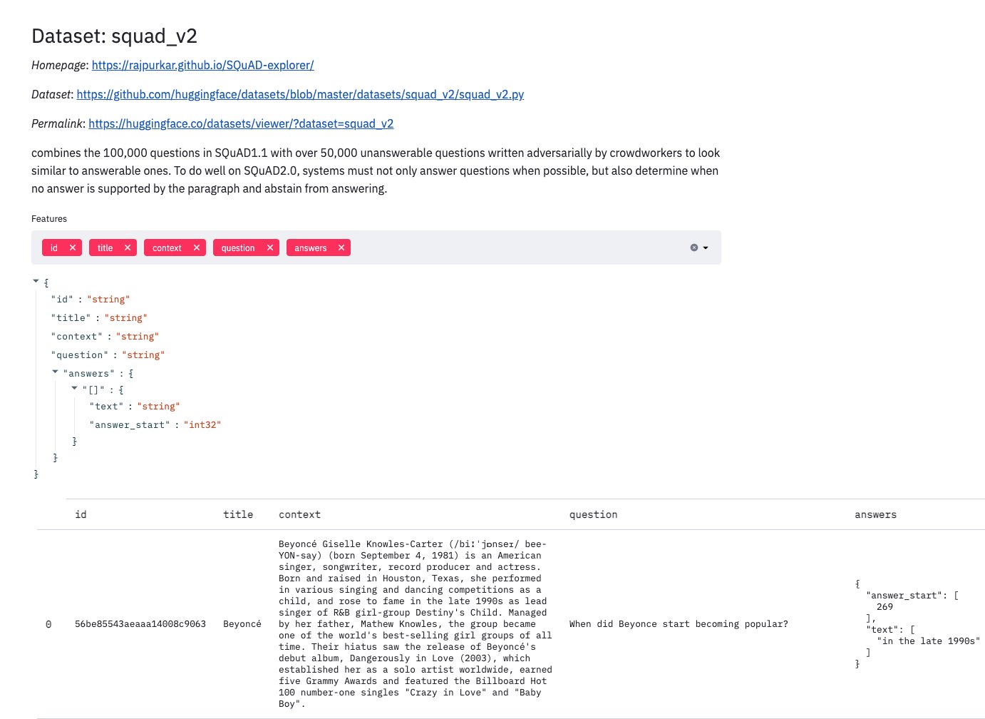
Our features are as follows:

  • ID – The ID of the text
  • title – The associated title for the topic
  • context – The context statement the model must search to find an answer
  • question – The question the model is being asked
  • answer – The accepted answer text and location in the context statement

Hugging Face datasets easily allow us to define this schema:

squad_dataset = Dataset.from_dict(dataset_dict,
features=datasets.Features(
    {
    "id": datasets.Value("string"),
    "title": datasets.Value("string"),
    "context": datasets.Value("string"),
    "question": datasets.Value("string"),
    "answers": datasets.features.Sequence(
        {
        "text": datasets.Value("string"),
        "answer_start": datasets.Value("int32"),
        }
    ),
    # These are the features of your dataset like images, labels ...
    }
))

After we create our dataset object, we have to tokenize the text. Because models can’t accept raw text as an input, we need to convert our text into a numeric input that it can understand, otherwise known as tokenization. Tokenization is model specific, so let’s understand the model we’re going to fine-tune. We’re using a distilbert-base-uncased model. It looks very similar to BERT: it uses input embeddings, multi-head attention (for more information about this operation, refer to The Illustrated Transformer), and feed forward layers, but has half the parameters of the original BERT base model. See the following initial model layers:
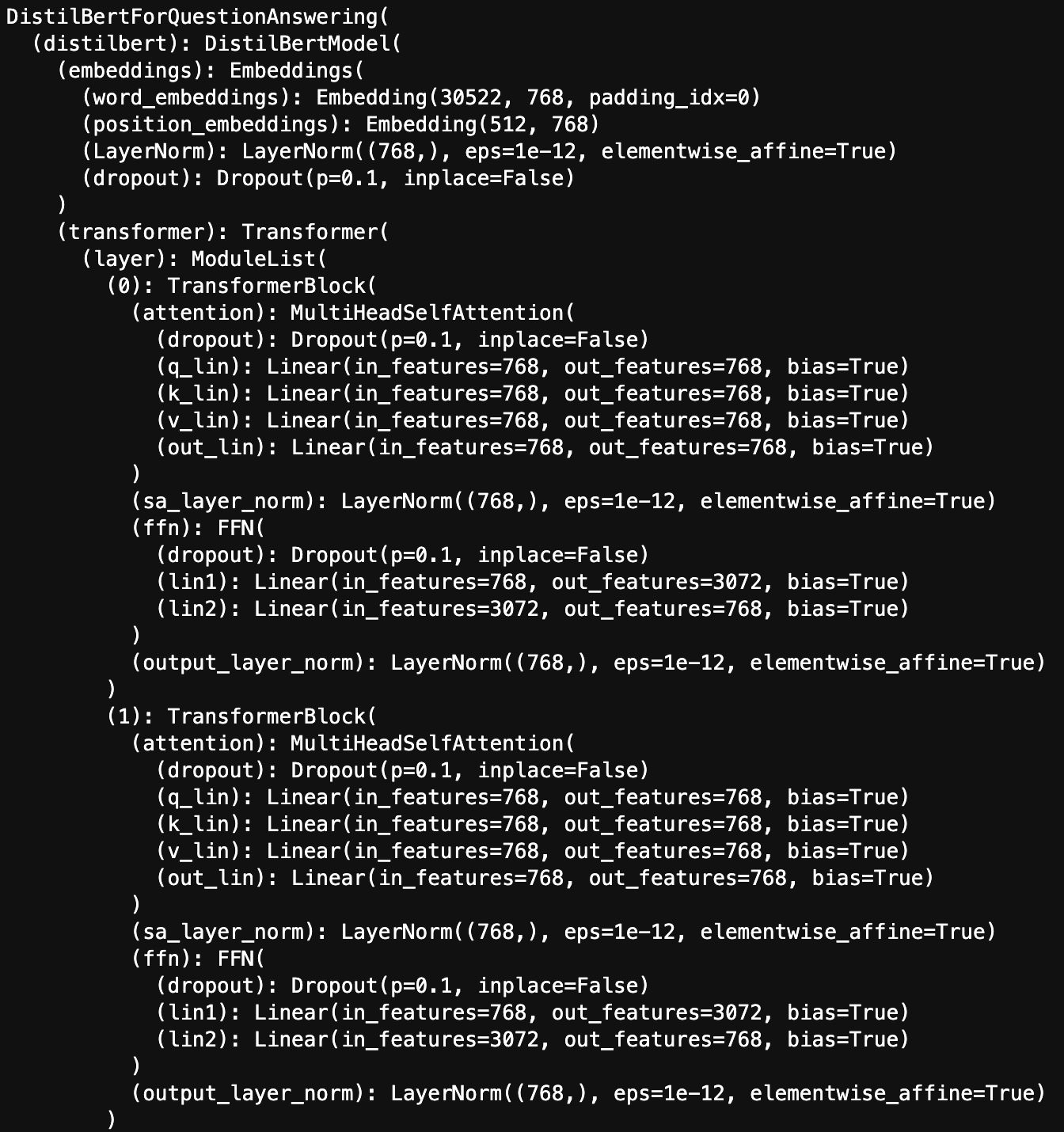
Let’s break down each component of the model’s title. The name distilbert denotes the fact that this is a distilled version of the BERT base model, which is obtained through a process called knowledge distillation. Knowledge distillation allows us to train a smaller student model on not only the training data but also the responses to the same training set from a larger pre-trained teacher model. base refers to the size of the model, in this case the model was distilled from a BERT base model (as opposed to a BERT large model). uncased refers to the text it was trained on. In this case the text didn’t account for case; all the text it was trained on was lowercase. The uncased aspect directly affects the way we tokenize our text. Thankfully, in addition to providing easy access to downloading transformer models, Hugging Face also provides the model’s accompanying tokenizer. We also downloaded a customized tokenizer for our distilbert-base-uncased model that we now use to transform our text:

# loadbase_model_prefix 
model_name = "distilbert-base-uncased"

# Load model & tokenizer
model = AutoModelForQuestionAnswering.from_pretrained(model_name)
tokenizer = AutoTokenizer.from_pretrained(model_name)
# set model to evaluation mode
evl = model.eval()

Another feature of the dataset class is it allows us to run preprocessing and tokenization in parallel with its map function. We define a processing function and then pass it to the map method.

For question answering, Hugging Face needs several components (which are also defined in the glossary):

  • attention mask – A mask indicating to the model which tokens to pay attention to, used primarily for differentiating between actual text and padding tokens
  • start_positions – The start position of the answer in the text
  • end_positions – The end position of the answer in the text
  • input_ids – The token indices mapping the tokens to the vocabulary

Our tokenizer will tokenize the text, but we need to explicitly capture the start and end positions of our answer, which is why we have defined a custom preprocessing function. Now that we have our inputs ready, let’s start training!

Launch training job

We can run training in our notebook, but the types of instances we need to train our Q&A model in a reasonable amount of time, p3 and p4 instances, are rather powerful. These instances tend to be overkill for running a notebook or as a persistent Amazon Elastic Compute Cloud (Amazon EC2) instance. This is where SageMaker training comes in. SageMaker training allows you to launch a training job on a specified instance or instances that are only up for the duration of the training job. This allows us to run on larger instances like the p4d.24xlarge, with 8 NVIDIA A100 GPUs, but without worrying about running up a huge bill in case we forget to turn it off. It also gives us easy access to other SageMaker functionalities, like SageMaker Experiments for tracking your ML training runs and SageMaker Debugger for understanding and profiling your training jobs.

Local training

Let’s start by understanding how training a model in Hugging Face works locally, then go over the adjustments we make to run it in SageMaker.

Hugging Face makes training easy through the use of their trainer class. The trainer class allows us to pass in our model, our train and validation datasets, our hyperparameters, and even our tokenizer. Because we already have our model as well as our training and validation sets, we only need to define our hyperparameters. We can do this through the TrainingArguments class. This allows us to specify things like the learning rate, batch size, number of epochs, and more in-depth parameters like weight decay or a learning rate scheduling strategy. After we define our TrainingArguments, we can pass in our model, training set, validation set, and arguments to instantiate our trainer class. Then we can simply call trainer.train() to start training our model. The following code block demonstrates how to run local training:

doc_stride=128
max_length=512
tokenized_train = squad_dataset.map(prepare_train_features, batched=True, remove_columns=squad_dataset.column_names, fn_kwargs = {'tokenizer':tokenizer, 'max_length':max_length, 'doc_stride':doc_stride})
tokenized_test = squad_test.map(prepare_train_features, batched=True, remove_columns=squad_test.column_names, fn_kwargs = {'tokenizer':tokenizer, 'max_length':max_length, 'doc_stride':doc_stride})

hf_args = TrainingArguments(
    'test_local',
    evaluation_strategy = "epoch",
    learning_rate=5e-5,
    per_device_train_batch_size=16,
    per_device_eval_batch_size=16,
    num_train_epochs=1,
    weight_decay=0.0001,
)

trainer = Trainer(
    model,
    hf_args,
    train_dataset=tokenized_train,
    eval_dataset=tokenized_test,
    data_collator=default_data_collator,
    tokenizer=tokenizer,
)

trainer.train()

Send data to S3

Doing the same thing in SageMaker training is straightforward. The first step is putting our data in Amazon S3 so that our model can access it. SageMaker training allows you to specify a data source; you can use sources like Amazon S3, Amazon Elastic File System (Amazon EFS), or Amazon FSx for Lustre for high-performance data ingestion. In our case, our augmented SQuAD dataset isn’t particularly large, so Amazon S3 is a good choice. We upload our training data to a folder in Amazon S3 and when SageMaker spins up our training instance, it downloads the data from our specified location.

Instantiate the model

To launch our training job, we can use the built-in Hugging Face estimator in the SageMaker SDK. SageMaker uses the estimator class to define the parameters for a training job as well as the number and type of instances to use for training. SageMaker training is built around the use of Docker containers. You can use the default containers in SageMaker or supply your own custom container for training. In the case of Hugging Face models, SageMaker has built-in Hugging Face containers with all the dependencies you need to run Hugging Face training jobs. All we need to do is define our training script, which our Hugging Face container uses as its entry point.

In this training script, we define our arguments, which we pass to our entry point in the form of a set of hyperparameters, as well as our training code. Our training code is the same as if we were running it locally; we can simply use the TrainingArguments and then pass them to a trainer object. The only difference is we need to specify the output location for our model to be in /opt/ml/model so that SageMaker training can take it, package it, and send it to Amazon S3. The following code block shows how to instantiate our Hugging Face estimator:

# hyperparameters, which are passed into the training job
hyperparameters={
    'model_name': model_name,
    'dataset_name':'squad',
    'do_train': True,
    'do_eval': True,
    'fp16': True,
    'train_batch_size': 32,
    'eval_batch_size': 32,
    'weight_decay':0.01,
    'warmup_steps':500,
    'learning_rate':5e-5,
    'epochs': 2,
    'max_length': 384,
    'max_steps': 100,
    'pad_to_max_length': True,
    'doc_stride': 128,
    'output_dir': '/opt/ml/model'
}

# estimator
huggingface_estimator = HuggingFace(entry_point='run_qa.py',
    source_dir='container_training',
    metric_definitions=metric_definitions,
    instance_type='ml.p3.8xlarge',
    instance_count=1,
    volume_size=100,
    role=role,
    transformers_version='4.4.2',
    pytorch_version='1.6.0',
    py_version='py36',
    hyperparameters = hyperparameters)

Fine-tune the model

For our specific training job, we use a p3.8xlarge instance consisting of 4 V100 GPUs. The trainer class automatically supports training on multi-GPU instances so we don’t need any additional setup to account for this. We train our model for two epochs, with a batch size of 16, and a learning rate of 4e5. We’re also enabling mixed precision training, which uses mixed precision in areas where we can reduce numerical precision without impacting our model’s accuracy. This increases our available memory and training speeds. To launch the training job, we call the fit method from our huggingface_estimator class.

huggingface_estimator.fit(data_channels, wait=False, job_name=f'hf-distilbert-squad-{int(time.time())}')

When our model is done training, we can download the model locally and load it into our notebook’s memory to test it, which is demonstrated in the notebook. We will focus on another option, deploying it as a SageMaker endpoint!

Deploy trained model

In addition to providing utilities for training, SageMaker can also allow data scientists and ML engineers to easily deploy REST endpoints for their trained models. You can deploy models trained in or outside of SageMaker. For more information, refer to Deploy a Model in Amazon SageMaker.

Because our model was trained in SageMaker, it’s already in the correct format to deploy as an endpoint. Similar to training, we define a SageMaker model class that defines the model, serving code, and the number and type of instances we want to deploy as endpoints. Also similar to training, serving is based on Docker containers, and we can use either of the built-in SageMaker containers or supply our own. For this post, we use a built-in PyTorch serving container, so we simply need to define a few things to get our endpoint up and running. Our serving code needs four functions:

  • model_fn – Defines how the endpoint loads the model (it only does this once, and then keeps it in memory for subsequent predictions)
  • input_fn – Defines how the input is deserialized and processed
  • predict_fn – Defines how our model makes predictions on our input
  • output_fn – Defines how the endpoint formats and sends back the output data to the client making the request

After we define these functions, we can deploy our endpoint and pass it context statements and questions and return its predicted answer:

endpoint_name = 'hf-distilbert-QA-string-endpoint4-185'
model_data = f"{huggingface_estimator.output_path}{huggingface_estimator.jobs[0].job_name}/output/model.tar.gz"

# We are going to use a SageMaker serving container
torch_model = PyTorchModel(model_data=model_data,
                           source_dir = 'container_serving',
                           role=role,
                          entry_point='transform_script.py',
                          framework_version='1.8.1',
                          py_version='py3',
                          predictor_cls = StringPredictor)
bert_end = torch_model.deploy(instance_type='ml.m5.2xlarge', initial_instance_count=1, #'ml.g4dn.xlarge'
                          endpoint_name=endpoint_name)

Visualize model results

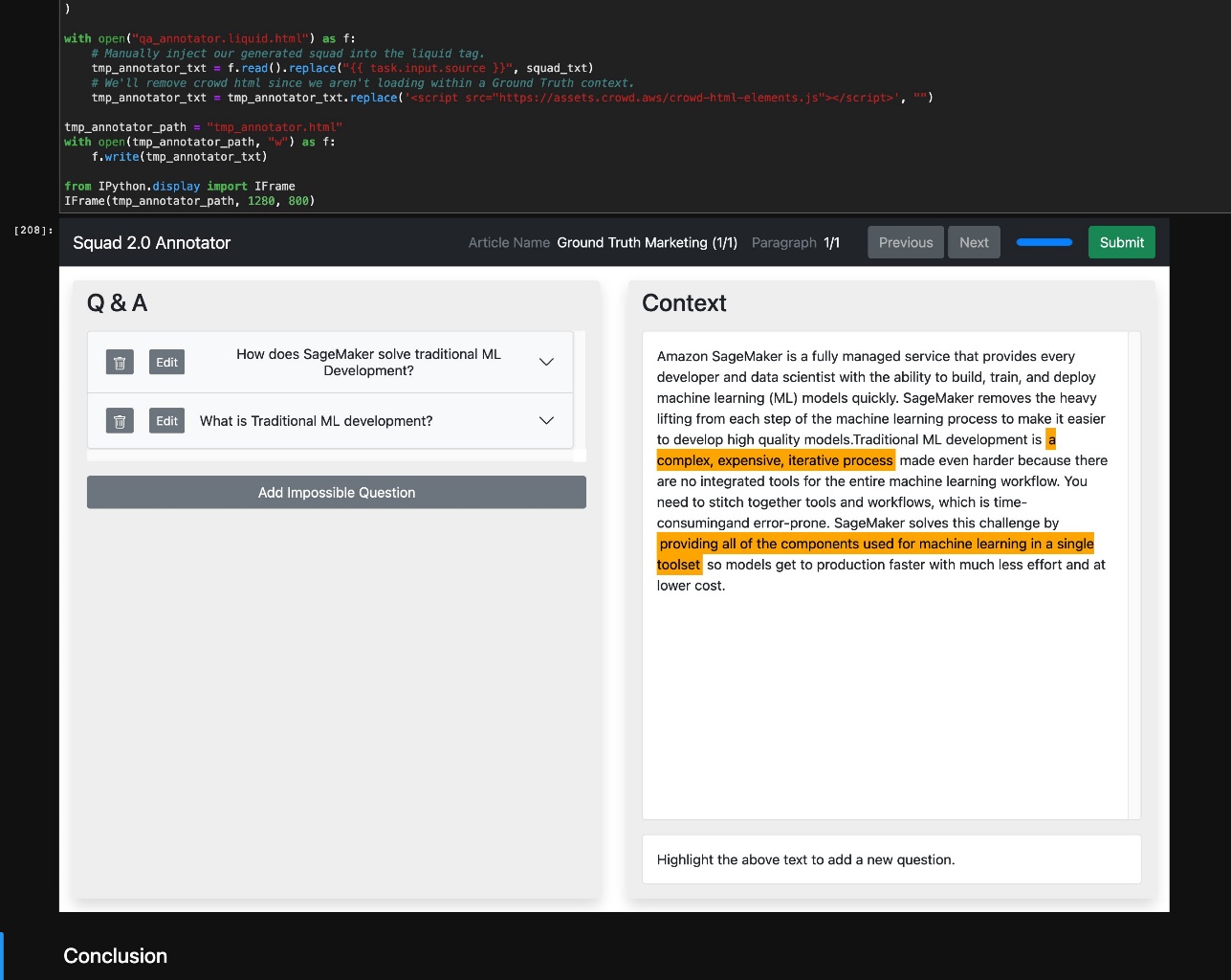
Because we deployed a SageMaker endpoint that allows us to send context statements and receive answers, we can go back and visualize the resulting inferences within the original SQuAD viewer to better visualize what our model found in the passage context. We do this by reformatting the results of inference back into SQuAD format, then replacing the Liquid tags in the worker template with the SQuAD-formatted JSON. We can then iframe the resulting UI inside our worker template to iteratively review results within the context of a single notebook, as shown in the following screenshot. Each question on the left can be clicked to highlight the spans of text on the right matching the query. With no question selected, all text spans are highlighted on the right as shown below.
Clean up

To avoid incurring future charges, run the Clean up section of the notebook to delete all the resources, including SageMaker endpoints, S3 objects that contains the raw and processed dataset, and the CloudFormation stack. When the deletion is complete, make sure to stop and delete the notebook instance that is hosting the current notebook script.

Conclusion

In this post, you learned how to create your own question answering dataset using Ground Truth and combine it with SQuAD to train and deploy your own question answering model using SageMaker. After you complete the notebook, you have a deployed SageMaker endpoint that was trained on your custom Q&A dataset. This endpoint is ready for integration into your production NLU workflows, because SageMaker endpoints are available through standard REST APIs. You also have an annotated custom dataset in SQuAD 2.0 format, which allows you to retrain your existing model or try training other question answering model architectures. Finally, you have a mechanism to quickly visualize the results from your inference by loading the worker template in your local notebook.

Try out the notebook, augment it with your own questions, and train and deploy your own custom question answering model for your NLU use cases!

Happy building!


About the Authors

Jeremy Feltracco is a Software Development Engineer with the Amazon ML Solutions Lab at Amazon Web Services. He uses his background in computer vision, robotics, and machine learning to help AWS customers accelerate their AI adoption.

Vidya Sagar Ravipati is a Manager at the Amazon ML Solutions Lab, where he leverages his vast experience in large-scale distributed systems and his passion for machine learning to help AWS customers across different industry verticals accelerate their AI and cloud adoption. Previously, he was a Machine Learning Engineer in Connectivity Services at Amazon who helped to build personalization and predictive maintenance platforms.

Isaac Privitera is a Senior Data Scientist at the Amazon Machine Learning Solutions Lab, where he develops bespoke machine learning and deep learning solutions to address customers’ business problems. He works primarily in the computer vision space, focusing on enabling AWS customers with distributed training and active learning.

Read More

Active offline policy selection

To make RL more applicable to real-world applications like robotics, we propose using an intelligent evaluation procedure to select the policy for deployment, called active offline policy selection (A-OPS). In A-OPS, we make use of the prerecorded dataset and allow limited interactions with the real environment to boost the selection quality.Read More

Use custom vocabulary in Amazon Lex to enhance speech recognition

In our daily conversations, we come across new words or terms that we may not know. Perhaps these are related to a new domain that we’re just getting familiar with, and we pick these up as we understand more about the domain. For example, home loan terminology (“curtailment”), shortened words, (“refi”, “comps”), and acronyms (“HELOC”) are likely new to first-time home buyers. Similarly, brand names can be tricky when you first hear of them. For example, with the sentence “I’d like to get a Cyetus 7601”, unless you’re a coffee aficionado, you may not realize the speaker is talking about a coffee machine brand. Some of these words may not be even present in the dictionary. Once we understand their usage, meaning, and spelling, they become part of our vocabulary so we can have effective conversations.

Similarly, bots have to understand and add such words to their vocabulary. Starting today, you can give Amazon Lex additional information about how to process speech input by creating a custom vocabulary. You can create a list with domain-specific words or brand names for improved speech recognition and end-user experience.

In this post, we review the custom vocabulary capability and use it for home loan customer service transactions and queries.

Overview of the custom vocabulary capability

You define the custom vocabulary for a language in the bot. In this case, we add brand names and domain-specific words and phrases in English (GB). The bot uses these phrases for transcription of speech input when it’s trying to understand the user’s request (or intent classification). You can also augment the custom vocabulary with information you have to collect (or slot elicitation) by configuring a setting on the slot type. You can specify the degree of boosting for each word or phrase by configuring a weight of 1, 2, or 3. We recommend you try out different weights. Words that are usually difficult to recognize or pronounce should have a higher weight.

The following is an example conversation with our bot:

Virtual Agent: Welcome to ACME bank. How can I help you?

Caller: Do you offer CapitaRise loans?

Virtual Agent: We offer CapitaRise loans for personal purposes. Do you want to get an application started?

Caller: No, thanks.

Virtual Agent: Is there anything else I can help you with today?

Caller: How about your refi rates?

Virtual Agent: For refinancing, we offer 4.5% with no closing costs for a 30 years fixed. Other information you might be interested in?

Caller: Yes, how about SBA?

Virtual Agent: We offer a variety of small business admin loans. You can find more information on our website. Anything else I can do for you?

Caller: I would like to do a payment on my HELOC.

Virtual Agent: To proceed with a payment, what is the account ID?

Caller: 1234

Virtual Agent: Thanks. What’s the payment amount?

Caller: 120

Virtual Agent: Thank you. The payment should be processed within 1 to 2 business days. Anything else I can help you with?

Caller: No, that’s it.

Virtual Agent: Thank you. Have a great day.

Solution overview

Let’s review the overall architecture for the solution (see the following diagram):

  • We use an Amazon Lex bot integrated with an Amazon Connect contact flow to deliver the conversational experience
  • We define the custom vocabulary for the English (GB) language by adding words such as “CapitaRise,” “HELOC,” and “refi”, along with weights
  • After the caller is authenticated, the control is passed to the bot to perform transactions (for example, to process payment)

The custom vocabulary file is a tab-separated list of values that contain the phrase to recognize and a weight to give the boost. Phrases with a higher boost value are more likely to be used when they appear in the audio input.

phrase	weight
CapitaRise	3
HELOC	2
Refi	2
S. B. A.	1

Deploy the sample Amazon Lex bot

To create the sample bot and configure the custom vocabulary, perform the following steps. This creates an Amazon Lex bot calledFinanceBot, with intents PersonalLoan, BusinessLoan, InterestRateRefinancing, InterestRateCredit, Payment, Welcome, and Goodbye, as well as two slot types (accountNumber and confirmationSlot).

  1. Download the Amazon Lex bot.
  2. On the Amazon Lex console, choose Actions, Import.
  3. Choose the file FinanceBot.zip file that you downloaded, and choose Import.
  4. In the IAM Permissions section, for Runtime role, choose Create a new role with basic Amazon Lex permissions.
  5. On the Amazon Lex console, navigate to the bot FinanceBot.
  6. Download the .zip file with the phrases that you want to add to the custom vocabulary.
  7. On the bot detail page, in the Add languages section, choose View languages.
  8. From the list of languages, choose English (GB).
  9. In the Custom vocabulary section, choose Import.
  10. Browse to the file to import, enter a password if necessary, and then choose Import.
  11. Choose Build.
  12. Download the supporting AWS Lambda code.
  13. On the Lambda console, create a new function and select Author from scratch.
  14. For Function name¸ enter FinanceBotEnglish.
  15. For Runtime, choose Python 3.8.
  16. Choose Create function.
  17. In the Code source section, open lambda_function.py and delete the existing code.
  18. Download the code and open it in a text editor.
  19. Copy and paste the code into the empty lambda_function.py tab.
  20. Choose Deploy.
  21. On the Amazon Lex console, and open FinanceBot.
  22. Choose Deployment and then Aliases, followed by TestBotAlias.
  23. On the Aliases page, in the Languages section, navigate to English (GB).
  24. For Source, select FinanceBotEnglish.
  25. For Lambda version or alias, enter $LATEST.
  26. On the Amazon Connect console, choose Contact flows.
  27. Download the contact flow to integrate with the Amazon Lex bot.
  28. In the Amazon Lex section, select your Amazon Lex bot and make it available for use in the Amazon Connect contact flows.
  29. Select the contact flow to load it into the application.
  30. Make sure the right bot is configured in the “Get Customer Input” block.
  31. Choose a queue in the “Set working queue” block.
  32. Add a phone number to the contact flow.
  33. Test the IVR flow by calling in to the phone number.

Test the solution

You can call in to the Amazon Connect phone number and interact with the bot.

Conclusion

Custom vocabulary enables improved recognition of domain-specific words and brand names for speech modality. You can easily define the custom vocabulary for your Amazon Lex bot and augment it to the bot definition. With improved recognition, you can enable more effective conversations across a broader set of use cases. You can configure custom vocabulary using the Amazon Lex V2 console or via the API. The capability is available for English (US) and English (GB) in all AWS Regions where Amazon Lex operates. To learn more, refer to custom vocabulary documentation.


About the Authors

Kai Loreck is a professional services Amazon Connect consultant. He works on designing and implementing scalable customer experience solutions. In his spare time, he can be found playing sports, snowboarding, or hiking in the mountains.

Anubhav Mishra is a Product Manager with AWS. He spends his time understanding customers and designing product experiences to address their business challenges.

Mebz Qazi is a Senior Consultant working on global projects for AWS. He very much enjoys working on technological innovation in natural language and AI/ML.

Sravan Bodapati is an Applied Science Manager at AWS Lex. He focuses on building cutting edge Artificial Intelligence and Machine Learning solutions for AWS customers in ASR and NLP space. In his spare time, he enjoys hiking, learning economics, watching TV shows and spending time with his family.

Read More

OpenAI Leadership Team Update

OpenAI Leadership Team Update

Greg Brockman is becoming President, a new role which reflects his unique combination of personal coding contributions on our critical path together with company strategy. He is currently focused on training our flagship AI systems.

Brad Lightcap has been pivotal in OpenAI’s growth, scaling our structure, team, and capital base through his oversight of our Finance, Legal, People, and Operations organizations. He will become Chief Operating Officer and expand his focus, working with our Applied AI teams to sharpen our business and commercial strategies. He will also continue to manage the OpenAI Startup Fund.

Mira Murati has done a tremendous job leading our research, product, and partnership functions over the past 18 months. Most recently, she was instrumental in bringing these functions together for the successful release of our DALL·E research. Mira is taking on the role of Chief Technology Officer, reflecting her leadership across these critical areas within OpenAI.

Chris Clark is becoming Head of Nonprofit and Strategic Initiatives. He will lead the operations of OpenAI’s nonprofit parent and key strategic projects including our relationships with mission-aligned partners.


These executives are supported by world-class teams who are the lifeblood of OpenAI, constantly advancing the state of the art in artificial intelligence research and deployment. It’s a pleasure to work alongside such incredible talent and leadership across our company. We are all very excited for the future. (And we’re hiring!)


OpenAI

Learning Locomotion Skills Safely in the Real World

The promise of deep reinforcement learning (RL) in solving complex, high-dimensional problems autonomously has attracted much interest in areas such as robotics, game playing, and self-driving cars. However, effectively training an RL policy requires exploring a large set of robot states and actions, including many that are not safe for the robot. This is a considerable risk, for example, when training a legged robot. Because such robots are inherently unstable, there is a high likelihood of the robot falling during learning, which could cause damage.

The risk of damage can be mitigated to some extent by learning the control policy in computer simulation and then deploying it in the real world. However, this approach usually requires addressing the difficult sim-to-real gap, i.e., the policy trained in simulation can not be readily deployed in the real world for various reasons, such as sensor noise in deployment or the simulator not being realistic enough during training. Another approach to solve this issue is to directly learn or fine-tune a control policy in the real world. But again, the main challenge is to assure safety during learning.

In “Safe Reinforcement Learning for Legged Locomotion”, we introduce a safe RL framework for learning legged locomotion while satisfying safety constraints during training. Our goal is to learn locomotion skills autonomously in the real world without the robot falling during the entire learning process. Our learning framework adopts a two-policy safe RL framework: a “safe recovery policy” that recovers robots from near-unsafe states, and a “learner policy” that is optimized to perform the desired control task. The safe learning framework switches between the safe recovery policy and the learner policy to enable robots to safely acquire novel and agile motor skills.

The Proposed Framework
Our goal is to ensure that during the entire learning process, the robot never falls, regardless of the learner policy being used. Similar to how a child learns to ride a bike, our approach teaches an agent a policy while using “training wheels”, i.e., a safe recovery policy. We first define a set of states, which we call a “safety trigger set”, where the robot is close to violating safety constraints but can still be saved by a safe recovery policy. For example, the safety trigger set can be defined as a set of states with the height of the robots being below a certain threshold and the roll, pitch, yaw angles being too large, which is an indication of falls. When the learner policy results in the robot being within the safety trigger set (i.e., where it is likely to fall), we switch to the safe recovery policy, which drives the robot back to a safe state. We determine when to switch back to the learner policy by leveraging an approximate dynamics model of the robot to predict the future robot trajectory. For example, based on the position of the robot’s legs and the current angle of the robot based on sensors for roll, pitch, and yaw, is it likely to fall in the future? If the predicted future states are all safe, we hand the control back to the learner policy, otherwise, we keep using the safe recovery policy.

The state diagram of the proposed approach. (1) If the learner policy violates the safety constraint, we switch to the safe recovery policy. (2) If the learner policy cannot ensure safety in the near future after switching to the safe recovery policy, we keep using the safe recovery policy. This allows the robot to explore more while ensuring safety.

This approach ensures safety in complex systems without resorting to opaque neural networks that may be sensitive to distribution shifts in application. In addition, the learner policy is able to explore states that are near safety violations, which is useful for learning a robust policy.

Because we use “approximated” dynamics to predict the future trajectory, we also examine how much safer a robot would be if we used a much more accurate model for its dynamics. We provide a theoretical analysis of this problem and show that our approach can achieve minimal safety performance loss compared to one with a full knowledge about the system dynamics.

Legged Locomotion Tasks
To demonstrate the effectiveness of the algorithm, we consider learning three different legged locomotion skills:

  1. Efficient Gait: The robot learns how to walk with low energy consumption and is rewarded for consuming less energy.
  2. Catwalk: The robot learns a catwalk gait pattern, in which the left and right two feet are close to each other. This is challenging because by narrowing the support polygon, the robot becomes less stable.
  3. Two-leg Balance: The robot learns a two-leg balance policy, in which the front-right and rear-left feet are in stance, and the other two are lifted. The robot can easily fall without delicate balance control because the contact polygon degenerates into a line segment.
Locomotion tasks considered in the paper. Top: efficient gait. Middle: catwalk. Bottom: two-leg balance.

Implementation Details
We use a hierarchical policy framework that combines RL and a traditional control approach for the learner and safe recovery policies. This framework consists of a high-level RL policy, which produces gait parameters (e.g., stepping frequency) and feet placements, and pairs it with a low-level process controller called model predictive control (MPC) that takes in these parameters and computes the desired torque for each motor in the robot. Because we do not directly command the motors’ angles, this approach provides more stable operation, streamlines the policy training due to a smaller action space, and results in a more robust policy. The input of the RL policy network includes the previous gait parameters, the height of the robot, base orientation, linear, angular velocities, and feedback to indicate whether the robot is approaching the safety trigger set. We use the same setup for each task.

We train a safe recovery policy with a reward for reaching stability as soon as possible. Furthermore, we design the safety trigger set with inspiration from capturability theory. In particular, the initial safety trigger set is defined to ensure that the robot’s feet can not fall outside of the positions from which the robot can safely recover using the safe recovery policy. We then fine-tune this set on the real robot with a random policy to prevent the robot from falling.

Real-World Experiment Results
We report the real-world experimental results showing the reward learning curves and the percentage of safe recovery policy activations on the efficient gait, catwalk, and two-leg balance tasks. To ensure that the robot can learn to be safe, we add a penalty when triggering the safe recovery policy. Here, all the policies are trained from scratch, except for the two-leg balance task, which was pre-trained in simulation because it requires more training steps.

Overall, we see that on these tasks, the reward increases, and the percentage of uses of the safe recovery policy decreases over policy updates. For instance, the percentage of uses of the safe recovery policy decreases from 20% to near 0% in the efficient gait task. For the two-leg balance task, the percentage drops from near 82.5% to 67.5%, suggesting that the two-leg balance is substantially harder than the previous two tasks. Still, the policy does improve the reward. This observation implies that the learner can gradually learn the task while avoiding the need to trigger the safe recovery policy. In addition, this suggests that it is possible to design a safe trigger set and a safe recovery policy that does not impede the exploration of the policy as the performance increases.

The reward learning curve (blue) and the percentage of safe recovery policy activations (red) using our safe RL algorithm in the real world.

In addition, the following video shows the learning process for the two-leg balance task, including the interplay between the learner policy and the safe recovery policy, and the reset to the initial position when an episode ends. We can see that the robot tries to catch itself when falling by putting down the lifted legs (front left and rear right) outward, creating a support polygon. After the learning episode ends, the robot walks back to the reset position automatically. This allows us to train policy autonomously and safely without human supervision.

Early training stage.
Late training stage.
Without a safe recovery policy.

Finally, we show the clips of learned policies. First, in the catwalk task, the distance between two sides of the legs is 0.09m, which is 40.9% smaller than the nominal distance. Second, in the two-leg balance task, the robot can maintain balance by jumping up to four times via two legs, compared to one jump from the policy pre-trained from simulation.

Final learned two-leg balance.

Conclusion
We presented a safe RL framework and demonstrated how it can be used to train a robotic policy with no falls and without the need for a manual reset during the entire learning process for the efficient gait and catwalk tasks. This approach even enables training of a two-leg balance task with only four falls. The safe recovery policy is triggered only when needed, allowing the robot to more fully explore the environment. Our results suggest that learning legged locomotion skills autonomously and safely is possible in the real world, which could unlock new opportunities including offline dataset collection for robot learning.

No model is without limitation. We currently ignore the model uncertainty from the environment and non-linear dynamics in our theoretical analysis. Including these would further improve the generality of our approach. In addition, some hyper-parameters of the switching criteria are currently being heuristically tuned. It would be more efficient to automatically determine when to switch based on the learning progress. Furthermore, it would be interesting to extend this safe RL framework to other robot applications, such as robot manipulation. Finally, designing an appropriate reward when incorporating the safe recovery policy can impact learning performance. We use a penalty-based approach that obtained reasonable results in these experiments, but we plan to investigate this in future work to make further performance improvements.

Acknowledgements
We would like to thank our paper co-authors: Tingnan Zhang, Linda Luu, Sehoon Ha, Jie Tan, and Wenhao Yu. We would also like to thank the team members of Robotics at Google for discussions and feedback.

Read More