3 Questions: How AI image generators could help robots

AI image generators, which create fantastical sights at the intersection of dreams and reality, bubble up on every corner of the web. Their entertainment value is demonstrated by an ever-expanding treasure trove of whimsical and random images serving as indirect portals to the brains of human designers. A simple text prompt yields a nearly instantaneous image, satisfying our primitive brains, which are hardwired for instant gratification. 

Although seemingly nascent, the field of AI-generated art can be traced back as far as the 1960s with early attempts using symbolic rule-based approaches to make technical images. While the progression of models that untangle and parse words has gained increasing sophistication, the explosion of generative art has sparked debate around copyright, disinformation, and biases, all mired in hype and controversy. Yilun Du, a PhD student in the Department of Electrical Engineering and Computer Science and affiliate of MIT’s Computer Science and Artificial Intelligence Laboratory (CSAIL), recently developed a new method that makes models like DALL-E 2 more creative and have better scene understanding. Here, Du describes how these models work, whether this technical infrastructure can be applied to other domains, and how we draw the line between AI and human creativity. 

Q: AI-generated images use something called “stable diffusion” models to turn words into astounding images in just a few moments. But for every image used, there’s usually a human behind it. So what’s the the line between AI and human creativity? How do these models really work? 

A: Imagine all of the images you could get on Google Search and their associated patterns. This is the diet these models are fed on. They’re trained on all of these images and their captions to generate images similar to the billions of images it has seen on the internet.

Let’s say a model has seen a lot of dog photos. It’s trained so that when it gets a similar text input prompt like “dog,” it’s able to generate a photo that looks very similar to the many dog pictures already seen. Now, more methodologically, how this all works dates back to a very old class of models called “energy-based models,” originating in the ’70’s or ’80’s.

In energy-based models, an energy landscape over images is constructed, which is used to simulate the physical dissipation to generate images. When you drop a dot of ink into water and it dissipates, for example, at the end, you just get this uniform texture. But if you try to reverse this process of dissipation, you gradually get the original ink dot in the water again. Or let’s say you have this very intricate block tower, and if you hit it with a ball, it collapses into a pile of blocks. This pile of blocks is then very disordered, and there’s not really much structure to it. To resuscitate the tower, you can try to reverse this folding process to generate your original pile of blocks.

The way these generative models generate images is in a very similar manner, where, initially, you have this really nice image, where you start from this random noise, and you basically learn how to simulate the process of how to reverse this process of going from noise back to your original image, where you try to iteratively refine this image to make it more and more realistic. 

In terms of what’s the line between AI and human creativity, you can say that these models are really trained on the creativity of people. The internet has all types of paintings and images that people have already created in the past. These models are trained to recapitulate and generate the images that have been on the internet. As a result, these models are more like crystallizations of what people have spent creativity on for hundreds of years. 

At the same time, because these models are trained on what humans have designed, they can generate very similar pieces of art to what humans have done in the past. They can find patterns in art that people have made, but it’s much harder for these models to actually generate creative photos on their own. 

If you try to enter a prompt like “abstract art” or “unique art” or the like, it doesn’t really understand the creativity aspect of human art. The models are, rather, recapitulating what people have done in the past, so to speak, as opposed to generating fundamentally new and creative art.

Since these models are trained on vast swaths of images from the internet, a lot of these images are likely copyrighted. You don’t exactly know what the model is retrieving when it’s generating new images, so there’s a big question of how you can even determine if the model is using copyrighted images. If the model depends, in some sense, on some copyrighted images, are then those new images copyrighted? That’s another question to address. 

Q: Do you believe images generated by diffusion models encode some sort of understanding about natural or physical worlds, either dynamically or geometrically? Are there efforts toward “teaching” image generators the basics of the universe that babies learn so early on? 

A: Do they understand, in code, some grasp of natural and physical worlds? I think definitely. If you ask a model to generate a stable configuration of blocks, it definitely generates a block configuration that’s stable. If you tell it, generate an unstable configuration of blocks, it does look very unstable. Or if you say “a tree next to a lake,” it’s roughly able to generate that. 

In a sense, it seems like these models have captured a large aspect of common sense. But the issue that makes us, still, very far away from truly understanding the natural and physical world is that when you try to generate infrequent combinations of words that you or I in our working our minds can very easily imagine, these models cannot.

For example, if you say, “put a fork on top of a plate,” that happens all the time. If you ask the model to generate this, it easily can. If you say, “put a plate on top of a fork,” again, it’s very easy for us to imagine what this would look like. But if you put this into any of these large models, you’ll never get a plate on top of a fork. You instead get a fork on top of a plate, since the models are learning to recapitulate all the images it’s been trained on. It can’t really generalize that well to combinations of words it hasn’t seen. 

A fairly well-known example is an astronaut riding a horse, which the model can do with ease. But if you say a horse riding an astronaut, it still generates a person riding a horse. It seems like these models are capturing a lot of correlations in the datasets they’re trained on, but they’re not actually capturing the underlying causal mechanisms of the world.

Another example that’s commonly used is if you get very complicated text descriptions like one object to the right of another one, the third object in the front, and a third or fourth one flying. It really is only able to satisfy maybe one or two of the objects. This could be partially because of the training data, as it’s rare to have very complicated captions But it could also suggest that these models aren’t very structured. You can imagine that if you get very complicated natural language prompts, there’s no manner in which the model can accurately represent all the component details.

Q: You recently came up with a new method that uses multiple models to create more complex images with better understanding for generative art. Are there potential applications of this framework outside of image or text domains? 

A: We were really inspired by one of the limitations of these models. When you give these models very complicated scene descriptions, they aren’t actually able to correctly generate images that match them. 

One thought is, since it’s a single model with a fixed computational graph, meaning you can only use a fixed amount of computation to generate an image, if you get an extremely complicated prompt, there’s no way you can use more computational power to generate that image.

If I gave a human a description of a scene that was, say, 100 lines long versus a scene that’s one line long, a human artist can spend much longer on the former. These models don’t really have the sensibility to do this. We propose, then, that given very complicated prompts, you can actually compose many different independent models together and have each individual model represent a portion of the scene you want to describe.

We find that this enables our model to generate more complicated scenes, or those that more accurately generate different aspects of the scene together. In addition, this approach can be generally applied across a variety of different domains. While image generation is likely the most currently successful application, generative models have actually been seeing all types of applications in a variety of domains. You can use them to generate different diverse robot behaviors, synthesize 3D shapes, enable better scene understanding, or design new materials. You could potentially compose multiple desired factors to generate the exact material you need for a particular application.

One thing we’ve been very interested in is robotics. In the same way that you can generate different images, you can also generate different robot trajectories (the path and schedule), and by composing different models together, you are able to generate trajectories with different combinations of skills. If I have natural language specifications of jumping versus avoiding an obstacle, you could also compose these models together, and then generate robot trajectories that can both jump and avoid an obstacle . 

In a similar manner, if we want to design proteins, we can specify different functions or aspects — in an analogous manner to how we use language to specify the content of the images — with language-like descriptions, such as the type or functionality of the protein. We could then compose these together to generate new proteins that can potentially satisfy all of these given functions. 

We’ve also explored using diffusion models on 3D shape generation, where you can use this approach to generate and design 3D assets. Normally, 3D asset design is a very complicated and laborious process. By composing different models together, it becomes much easier to generate shapes such as, “I want a 3D shape with four legs, with this style and height,” potentially automating portions of 3D asset design. 

Read More

Amazon SageMaker Automatic Model Tuning now supports grid search

Today Amazon SageMaker announced the support of Grid search for automatic model tuning, providing users with an additional strategy to find the best hyperparameter configuration for your model.

Amazon SageMaker automatic model tuning finds the best version of a model by running many training jobs on your dataset using a range of hyperparameters that you specify. Then it chooses the hyperparameter values that result in a model that performs the best, as measured by a metric of your choice.

To find the best hyperparameters values for your model, Amazon SageMaker automatic model tuning supports multiple strategies, including Bayesian (default), Random search, and Hyperband.

Grid search

Grid search exhaustively explores the configurations in the grid of hyperparameters that you define, which allows you to get insights into the most promising hyperparameter configurations in your grid and deterministically reproduce your results across different tuning runs. Grid search gives you more confidence that the entire hyper parameter search space was explored. This benefit comes with a trade-off because it’s computationally more expensive than Bayesian and random search if your main goal is to find the best hyperparameter configuration.

Grid search with Amazon SageMaker

In Amazon SageMaker, you use Grid search when your problem requires you to have the optimal hyperparameter combination that maximizes or minimizes your objective metric. A common use case where customer use Grid Search is when model accuracy and reproducibility is more important for your business than the training cost required to obtain it.

To enable Grid Search in Amazon SageMaker, set the Strategy field to Grid when you create a tuning job, as follows:

{
    "ParameterRanges": {...}
    "Strategy": "Grid",
    "HyperParameterTuningJobObjective": {...}
}

Additionally, Grid search requires you to define your search space (Cartesian grid) as a categorical range of discrete values in your job definition using the CategoricalParameterRanges key under the ParameterRanges parameter, as follows:

{
    "ParameterRanges": {
        "CategoricalParameterRanges": [
 {
              "Name": "eta", "Values": ['0.1', '0.2', '0.3', '0.4', '0.5']
            },
            {
              "Name": "alpha", "Values": ['0.1', '0.2']
            },
        ],

    },
    ...
}

Note that we don’t specify MaxNumberOfTrainingJobs for Grid search in the job definition because this is determined for you from the number of category combinations. When using Random and Bayesian search, you specify the MaxNumberOfTrainingJobs parameter as a way to control tuning job cost by defining an upper boundary for compute. With Grid search, the value of MaxNumberOfTrainingJobs (now optional) is automatically set as the number of candidates for the grid search in the DescribeHyperParameterTuningJob shape. This allows you to explore your desired grid of hyperparameters exhaustively. Additionally, Grid search job definition only accepts discrete categorical ranges and doesn’t require a continuous or integer ranges definition because each value in the grid is considered discrete.

Grid Search experiment

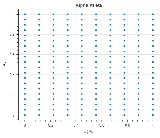
In this experiment, given a regression task, we search for the optimal hyperparameters within a search space of 200 hyperparameters, 20 eta and 10 alpha ranging from 0.1 to 1. We use the direct marketing dataset to tune a regression model.

  • eta: Step size shrinkage used in updates to prevent over-fitting. After each boosting step, you can directly get the weights of new features. The eta parameter actually shrinks the feature weights to make the boosting process more conservative.
  • alpha: L1 regularization term on weights. Increasing this value makes models more conservative.

The chart to the left shows an analysis of the eta hyperparameter in relation to the objective metric and demonstrates how grid search has exhausted the entire search space (grid) in the X axes before returning the best model. Equally, the chart to the right analyzes the two hyperparameters in a single cartesian space to demonstrate that all the points in the grid were picked during tuning.

The experiment above demonstrates that the exhaustive nature of Grid search guaranties an optimal hyperparameter selection given the defined search space. It also demonstrates that you can reproduce your search result across tuning iterations, all other things being equal.

Amazon SageMaker Automatic Model Tuning workflows (AMT)

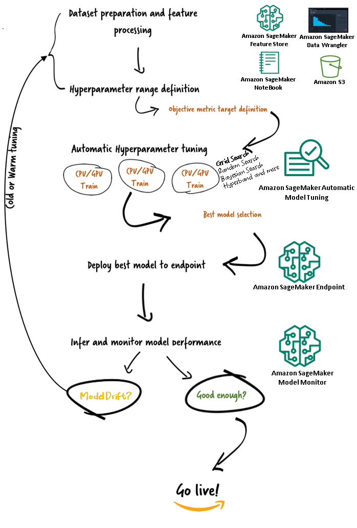
With Amazon SageMaker automatic model tuning, you can find the best version of your model by running training jobs on your dataset with several search strategies, such as Bayesian, Random search, Grid search, and Hyperband. Automatic model tuning allows you to reduce the time to tune a model by automatically searching for the best hyperparameter configuration within the hyperparameter ranges that you specify.

Now that we have reviewed the advantage of using Grid search in Amazon SageMaker AMT, let’s take a look at AMT’s workflows and understand how it all fits together in SageMaker.

Conclusion

In this post, we discussed how you can now use the Grid search strategy to find the best model and its ability to deterministically reproduce results across different tuning jobs. We discussed the trade-off when using grid search compared to other strategies, and how it allows you to explore what regions of the hyperparameter spaces are most promising and reproduce your results deterministically.

To learn more about automatic model tuning, visit the product page and technical documentation.


About the author

Doug Mbaya is a Senior Partner Solution architect with a focus in data and analytics. Doug works closely with AWS partners, helping them integrate data and analytics solutions in the cloud.

Read More

Natural Language Assessment: A New Framework to Promote Education

Natural Language Assessment: A New Framework to Promote Education

Whether it’s a professional honing their skills or a child learning to read, coaches and educators play a key role in assessing the learner’s answer to a question in a given context and guiding them towards a goal. These interactions have unique characteristics that set them apart from other forms of dialogue, yet are not available when learners practice alone at home. In the field of natural language processing, this type of capability has not received much attention and is technologically challenging. We set out to explore how we can use machine learning to assess answers in a way that facilitates learning.

In this blog, we introduce an important natural language understanding (NLU) capability called Natural Language Assessment (NLA), and discuss how it can be helpful in the context of education. While typical NLU tasks focus on the user’s intent, NLA allows for the assessment of an answer from multiple perspectives. In situations where a user wants to know how good their answer is, NLA can offer an analysis of how close the answer is to what is expected. In situations where there may not be a “correct” answer, NLA can offer subtle insights that include topicality, relevance, verbosity, and beyond. We formulate the scope of NLA, present a practical model for carrying out topicality NLA, and showcase how NLA has been used to help job seekers practice answering interview questions with Google’s new interview prep tool, Interview Warmup.

Overview of Natural Language Assessment (NLA)

The goal of NLA is to evaluate the user’s answer against a set of expectations. Consider the following components for an NLA system interacting with students:

  • A question presented to the student
  • Expectations that define what we expect to find in the answer (e.g., a concrete textual answer, a set of topics we expect the answer to cover, conciseness)
  • An answer provided by the student
  • An assessment output (e.g., correctness, missing information, too specific or general, stylistic feedback, pronunciation, etc.)
  • [Optional] A context (e.g., a chapter in a book or an article)

With NLA, both the expectations about the answer and the assessment of the answer can be very broad. This enables teacher-student interactions that are more expressive and subtle. Here are two examples:

  1. A question with a concrete correct answer: Even in situations where there is a clear correct answer, it can be helpful to assess the answer more subtly than simply correct or incorrect. Consider the following:

    Context: Harry Potter and the Philosopher’s Stone
    Question: “What is Hogwarts?”
    Expectation: “Hogwarts is a school of Witchcraft and Wizardry” [expectation is given as text]
    Answer: “I am not exactly sure, but I think it is a school.”

    The answer may be missing salient details but labeling it as incorrect wouldn’t be entirely true or useful to a user. NLA can offer a more subtle understanding by, for example, identifying that the student’s answer is too general, and also that the student is uncertain.

    Illustration of the NLA process from input question, answer and expectation to assessment output.

    This kind of subtle assessment, along with noting the uncertainty the student expressed, can be important in helping students build skills in conversational settings.

  2. Topicality expectations: There are many situations in which a concrete answer is not expected. For example, if a student is asked an opinion question, there is no concrete textual expectation. Instead, there’s an expectation of relevance and opinionation, and perhaps some level of succinctness and fluency. Consider the following interview practice setup:

    Question: “Tell me a little about yourself?”
    Expectations: { “Education”, “Experience”, “Interests” } (a set of topics)
    Answer: “Let’s see. I grew up in the Salinas valley in California and went to Stanford where I majored in economics but then got excited about technology so next I ….”

    In this case, a useful assessment output would map the user’s answer to a subset of the topics covered, possibly along with a markup of which parts of the text relate to which topic. This can be challenging from an NLP perspective as answers can be long, topics can be mixed, and each topic on its own can be multi-faceted.

A Topicality NLA Model

In principle, topicality NLA is a standard multi-class task for which one can readily train a classifier using standard techniques. However, training data for such scenarios is scarce and it would be costly and time consuming to collect for each question and topic. Our solution is to break each topic into granular components that can be identified using large language models (LLMs) with a straightforward generic tuning.

We map each topic to a list of underlying questions and define that if the sentence contains an answer to one of those underlying questions, then it covers that topic. For the topic “Experience” we might choose underlying questions such as:

  • Where did you work?
  • What did you study?

While for the topic “Interests” we might choose underlying questions such as:

  • What are you interested in?
  • What do you enjoy doing?

These underlying questions are designed through an iterative manual process. Importantly, since these questions are sufficiently granular, current language models (see details below) can capture their semantics. This allows us to offer a zero-shot setting for the NLA topicality task: once trained (more on the model below), it is easy to add new questions and new topics, or adapt existing topics by modifying their underlying content expectation without the need to collect topic specific data. See below the model’s predictions for the sentence “I’ve worked in retail for 3 years” for the two topics described above:

A diagram of how the model uses underlying questions to predict the topic most likely to be covered by the user’s answer.

Since an underlying question for the topic “Experience” was matched, the sentence would be classified as “Experience”.

Application: Helping Job Seekers Prepare for Interviews

Interview Warmup is a new tool developed in collaboration with job seekers to help them prepare for interviews in fast-growing fields of employment such as IT Support and UX Design. It allows job seekers to practice answering questions selected by industry experts and to become more confident and comfortable with interviewing. As we worked with job seekers to understand their challenges in preparing for interviews and how an interview practice tool could be most useful, it inspired our research and the application of topicality NLA.

We build the topicality NLA model (once for all questions and topics) as follows: we train an encoder-only T5 model (EncT5 architecture) with 350 million parameters on Question-Answers data to predict the compatibility of an <underlying question, answer> pair. We rely on data from SQuAD 2.0 which was processed to produce <question, answer, label> triplets.

In the Interview Warmup tool, users can switch between talking points to see which ones were detected in their answer.

The tool does not grade or judge answers. Instead it enables users to practice and identify ways to improve on their own. After a user replies to an interview question, their answer is parsed sentence-by-sentence with the Topicality NLA model. They can then switch between different talking points to see which ones were detected in their answer. We know that there are many potential pitfalls in signaling to a user that their response is “good”, especially as we only detect a limited set of topics. Instead, we keep the control in the user’s hands and only use ML to help users make their own discoveries about how to improve.

So far, the tool has had great results helping job seekers around the world, including in the US, and we have recently expanded it to Africa. We plan to continue working with job seekers to iterate and make the tool even more helpful to the millions of people searching for new jobs.

A short film showing how Interview Warmup and its NLA capabilities were developed in collaboration with job seekers.

Conclusion

Natural Language Assessment (NLA) is a technologically challenging and interesting research area. It paves the way for new conversational applications that promote learning by enabling the nuanced assessment and analysis of answers from multiple perspectives. Working together with communities, from job seekers and businesses to classroom teachers and students, we can identify situations where NLA has the potential to help people learn, engage, and develop skills across an array of subjects, and we can build applications in a responsible way that empower users to assess their own abilities and discover ways to improve.

Acknowledgements

This work is made possible through a collaboration spanning several teams across Google. We’d like to acknowledge contributions from Google Research Israel, Google Creative Lab, and Grow with Google teams among others.

Read More

A new genome sequencing tool powered with our technology

A new genome sequencing tool powered with our technology

Genome sequencing provides a more complete description of cells and organisms, allowing scientists to uncover serious genetic conditions such as the elevated risk for breast cancer or pulmonary arterial hypertension. While researching genomics has the potential to save lives and preserve people’s quality of life, it’s incredibly challenging work.

Back in January, we announced a partnership with PacBio, a developer of genome sequencing instruments, to further advance genomic technologies. Today, PacBio is introducing the Revio sequencing system, an instrument that runs on our deep learning technology, DeepConsensus. With DeepConsensus built right into Revio, researchers can quickly and accurately identify genetic variants that cause diseases.

How Google Health’s technology works

Genome sequencing requires observing individual DNA molecules amidst a complex and noisy background. To address the problem, Google Health worked to adapt Transformer, one of our most influential existing deep learning methods that was developed in 2017 primarily to understand languages. We then applied it to PacBio’s data, which uses fluorescence light to encode DNA sequences. The result was DeepConsensus.

Last year, we demonstrated that DeepConsensus was capable of reducing sequencing errors by 42%, resulting in better genome assemblies and more accurate identification of genetic variants. Although this was a promising research demonstration, we knew that DeepConsensus could have the greatest impact if it was running directly on PacBio’s sequencing instrument. Over the last year, we’ve worked closely with PacBio to speed up DeepConsensus by over 500x from its initial release. We’ve also further improved its accuracy to reduce errors by 59%.

Combining our AI methods and genomics work with PacBio’s instruments and expertise, we were able to build better methods for the research community. Our partnership with PacBio doesn’t stop with Revio. There’s limitless potential to make an impact on the research community and improve healthcare and access for people around the world.

Read More

Introducing the Amazon SageMaker Serverless Inference Benchmarking Toolkit

Amazon SageMaker Serverless Inference is a purpose-built inference option that makes it easy for you to deploy and scale machine learning (ML) models. It provides a pay-per-use model, which is ideal for services where endpoint invocations are infrequent and unpredictable. Unlike a real-time hosting endpoint, which is backed by a long-running instance, compute resources for serverless endpoints are provisioned on demand, thereby eliminating the need to choose instance types or manage scaling policies.

The following high-level architecture illustrates how a serverless endpoint works. A client invokes an endpoint, which is backed by AWS managed infrastructure.

However, serverless endpoints are prone to cold starts in the order of seconds, and is therefore more suitable for intermittent or unpredictable workloads.

To help determine whether a serverless endpoint is the right deployment option from a cost and performance perspective, we have developed the SageMaker Serverless Inference Benchmarking Toolkit, which tests different endpoint configurations and compares the most optimal one against a comparable real-time hosting instance.

In this post, we introduce the toolkit and provide an overview of its configuration and outputs.

Solution overview

You can download the toolkit and install it from the GitHub repo. Getting started is easy: simply install the library, create a SageMaker model, and provide the name of your model along with a JSON lines formatted file containing a sample set of invocation parameters, including the payload body and content type. A convenience function is provided to convert a list of sample invocation arguments to a JSON lines file or a pickle file for binary payloads such as images, video, or audio.

Install the toolkit

First install the benchmarking library into your Python environment using pip:

pip install sm-serverless-benchmarking

You can run the following code from an Amazon SageMaker Studio instance, SageMaker notebook instance, or any instance with programmatic access to AWS and the appropriate AWS Identity and Access Management (IAM) permissions. The requisite IAM permissions are documented in the GitHub repo. For additional guidance and example policies for IAM, refer to How Amazon SageMaker Works with IAM. This code runs a benchmark with a default set of parameters on a model that expects a CSV input with two example records. It’s a good practice to provide a representative set of examples to analyze how the endpoint performs with different input payloads.

from sm_serverless_benchmarking import benchmark
from sm_serverless_benchmarking.utils import convert_invoke_args_to_jsonl
model_name = "<SageMaker Model Name>"
example_invoke_args = [
        {'Body': '1,2,3,4,5', "ContentType": "text/csv"},
        {'Body': '6,7,8,9,10', "ContentType": "text/csv"}
        ]
example_args_file = convert_invoke_args_to_jsonl(example_invoke_args,
output_path=".")
r = benchmark.run_serverless_benchmarks(model_name, example_args_file)

Additionally, you can run the benchmark as a SageMaker Processing job, which may be a more reliable option for longer-running benchmarks with a large number of invocations. See the following code:

from sm_serverless_benchmarking.sagemaker_runner import run_as_sagemaker_job
run_as_sagemaker_job(
                    role="<execution_role_arn>",
                    model_name="<model_name>",
                    invoke_args_examples_file="<invoke_args_examples_file>",
                    )

Note that this will incur additional cost of running an ml.m5.large SageMaker Processing instance for the duration of the benchmark.

Both methods accept a number of parameters to configure, such as a list of memory configurations to benchmark and the number of times each configuration will be invoked. In most cases, the default options should suffice as a starting point, but refer to the GitHub repo for a complete list and descriptions of each parameter.

Benchmarking configuration

Before delving into what the benchmark does and what outputs it produces, it’s important to understand a few key concepts when it comes to configuring serverless endpoints.

There are two key configuration options: MemorySizeInMB and MaxConcurrency. MemorySizeInMB configures the amount of memory that is allocated to the instance, and can be 1024 MB, 2048 MB, 3072 MB, 4096 MB, 5120 MB, or 6144 MB. The number of vCPUs also scales proportionally to the amount of memory allocated. The MaxConcurrency parameter adjusts how many concurrent requests an endpoint is able to service. With a MaxConcurrency of 1, a serverless endpoint can only process a single request at a time.

To summarize, the MemorySizeInMB parameter provides a mechanism for vertical scalability, allowing you to adjust memory and compute resources to serve larger models, whereas MaxConcurrency provides a mechanism for horizontal scalability, allowing your endpoint to process more concurrent requests.

The cost of operating an endpoint is largely determined by the memory size, and there is no cost associated with increasing the max concurrency. However, there is a per-Region account limit for max concurrency across all endpoints. Refer to SageMaker endpoints and quotas for the latest limits.

Benchmarking outputs

Given this, the goal of benchmarking a serverless endpoint is to determine the most cost-effective and reliable memory size setting, and the minimum max concurrency that can handle your expected traffic patterns.

By default, the tool runs two benchmarks. The first is a stability benchmark, which deploys an endpoint for each of the specified memory configurations and invokes each endpoint with the provided sample payloads. The goal of this benchmark is to determine the most effective and stable MemorySizeInMB setting. The benchmark captures the invocation latencies and computes the expected per-invocation cost for each endpoint. It then compares the cost against a similar real-time hosting instance.

When the benchmarking is complete, the tool generates several outputs in the specified result_save_path directory with the following directory structure:

├── benchmarking_report
├── concurrency_benchmark_raw_results
├── concurrency_benchmark_summary_results
├── cost_analysis_summary_results
├── stability_benchmark_raw_results
├── stability_benchmark_summary_results

The benchmarking_report directory contains a consolidated report with all the summary outputs that we outline in this post. Additional directories contain raw and intermediate outputs that you can use for additional analyses. Refer to the GitHub repo for a more detailed description of each output artifact.

Let’s examine a few actual benchmarking outputs for an endpoint serving a computer vision MobileNetV2 TensorFlow model. If you’d like to reproduce this example, refer to the example notebooks directory in the GitHub repo.

The first output within the consolidated report is a summary table that provides the minimum, mean, medium, and maximum latency metrics for each MemorySizeInMB successful memory size configuration. As shown in the following table, the average invocation latency (invocation_latency_mean) continued to improve as memory configuration was increased to 3072 MB, but stopped improving thereafter.

In addition to the high-level descriptive statistics, a chart is provided showing the distribution of latency as observed from the client for each of the memory configurations. Again, we can observe that the 1024 MB configuration isn’t as performant as the other options, but there isn’t a substantial difference in performance in configurations of 2048 and above.

Amazon CloudWatch metrics associated with each endpoint configuration are also provided. One key metric here is ModelSetupTime, which measures how long it took to load the model when the endpoint was invoked in a cold state. The metric may not always appear in the report as an endpoint is launched in a warm state. A cold_start_delay parameter is available for specifying the number of seconds to sleep before starting the benchmark on a deployed endpoint. Setting this parameter to a higher number such as 600 seconds should increase the likelihood of a cold state invocation and improve the chances of capturing this metric. Additionally, this metric is far more likely to be captured with the concurrent invocation benchmark, which we discuss later in this section.

The following table shows the metrics captured by CloudWatch for each memory configuration.

The next chart shows the performance and cost trade-offs of different memory configurations. One line shows the estimated cost of invoking the endpoint 1 million times, and the other shows the average response latency. These metrics can inform your decision of which endpoint configuration is most cost-effective. In this example, we see that the average latency flattens out after 2048 MB, whereas the cost continues to increase, indicating that for this model a memory size configuration of 2048 would be most optimal.

The final output of the cost and stability benchmark is a recommended memory configuration, along with a table comparing the cost of operating a serverless endpoint against a comparable SageMaker hosting instance. Based on the data collected, the tool determined that the 2048 MB configuration is the most optimal one for this model. Although the 3072 configuration provides roughly 10 milliseconds better latency, that comes with a 30% increase in cost, from $4.55 to $5.95 per 1 million requests. Additionally, the output shows that a serverless endpoint would provide savings of up to 88.72% against a comparable real-time hosting instance when there are fewer than 1 million monthly invocation requests, and breaks even with a real-time endpoint after 8.5 million requests.

The second type of benchmark is optional and tests various MaxConcurency settings under different traffic patterns. This benchmark is usually run using the optimal MemorySizeInMB configuration from the stability benchmark. The two key parameters for this benchmark is a list of MaxConcurency settings to test along with a list of client multipliers, which determine the number of simulated concurrent clients that the endpoint is tested with.

For example, by setting the concurrency_benchmark_max_conc parameter to [4, 8] and concurrency_num_clients_multiplier to [1, 1.5, 2], two endpoints are launched: one with MaxConcurency of 4 and the other 8. Each endpoint is then benchmarked with a (MaxConcurency x multiplier) number of simulated concurrent clients, which for the endpoint with a concurrency of 4 translates to load test benchmarks with 4, 6, and 8 concurrent clients.

The first output of this benchmark is a table that shows the latency metrics, throttling exceptions, and transactions per second metrics (TPS) associated with each MaxConcurrency configuration with different numbers of concurrent clients. These metrics help determine the appropriate MaxConcurrency setting to handle the expected traffic load. In the following table, we can see that an endpoint configured with a max concurrency of 8 was able to handle up to 16 concurrent clients with only two throttling exceptions out of 2,500 invocations made at an average of 24 transactions per second.

The next set of outputs provides a chart for each MaxConcurrency setting showing the distribution of latency under different loads. In this example, we can see that an endpoint with a MaxConcurrency setting of 4 was able to successfully process all requests with up to 8 concurrent clients with a minimal increase in invocation latency.

The final output provides a table with CloudWatch metrics for each MaxConcurrency configuration. Unlike the previous table showing the distribution of latency for each memory configuration, which may not always display the cold start ModelSetupTime metric, this metric is far more likely to appear in this table due to the larger number of invocation requests and a greater MaxConcurrency.

Conclusion

In this post, we introduced the SageMaker Serverless Inference Benchmarking Toolkit and provided an overview of its configuration and outputs. The tool can help you make a more informed decision with regards to serverless inference by load testing different configurations with realistic traffic patterns. Try the benchmarking toolkit with your own models to see for yourself the performance and cost saving you can expect by deploying a serverless endpoint. Please refer to the GitHub repo for additional documentation and example notebooks.

Additional resources


About the authors

Simon Zamarin is an AI/ML Solutions Architect whose main focus is helping customers extract value from their data assets. In his spare time, Simon enjoys spending time with family, reading sci-fi, and working on various DIY house projects.

Dhawal Patel is a Principal Machine Learning Architect at AWS. He has worked with organizations ranging from large enterprises to mid-sized startups on problems related to distributed computing and artificial intelligence. He focuses on deep learning, including NLP and computer vision domains. He helps customers achieve high-performance model inference on SageMaker.

Rishabh Ray Chaudhury is a Senior Product Manager with Amazon SageMaker, focusing on machine learning inference. He is passionate about innovating and building new experiences for machine learning customers on AWS to help scale their workloads. In his spare time, he enjoys traveling and cooking. You can find him on LinkedIn.

Read More

Jetson-Driven Grub Getter: Cartken Rolls Out Robots-as-a-Service for Deliveries

There’s a new sidewalk-savvy robot, and it’s delivering coffee, grub and a taste of fun.

The bot is garnering interest for Oakland, Calif., startup Cartken. The company, founded in 2019, has rapidly deployed robots for a handful of customer applications, including for Starbucks and Grubhub deliveries.

Cartken CEO Chris Bersch said that he and co-founders Jonas Witt, Jake Stelman and Anjali Jindal Naik got excited about the prospect for robots because of the technology’s readiness and affordability. The four Google alumni decided the timing was right to take the leap to start a company together.

“What we saw was a technological inflection point where we could make small self-driving vehicles work on the street,” said Bersch. “Because it doesn’t make sense to build a $20,000 robot that can deliver burritos.”

Cartken is among a surge of NVIDIA Jetson-enabled autonomous mobile robot (AMR) startups making advances across agtech, manufacturing, retail and last-mile delivery.

New and established companies are seeking business efficiencies as well as labor support amid ongoing shortages in the post-COVID era, driving market demand.

Revenue from robotic last-mile deliveries is expected to grow more than 9x to $670 million in 2030, up from $70 million in 2022, according to ABI Research.

Jetson Drives Robots as a Service 

Cartken offers robots as a service (RaaS) to customers in a pay-for-usage model. This way, as a white- label technology provider, Cartken enables companies to customize the robots for their particular brand appearance and specific application features.

It’s among a growing cohort of companies riding the RaaS wave, with ambitions as far flung as on-demand remote museum visits to autonomous industrial lawn mowers.

Much of this is made possible with the powerful NVIDIA Jetson embedded computing modules, which can handle a multitude of sensors and cameras.

“Cartken chose the Jetson edge AI platform because it offers superior embedded computational performance, which is needed to run Cartken’s advanced AI algorithms. In addition, the low energy consumption allows Cartken’s robots to run a whole day on a single battery charge,” said Bersch.

The company relies on the NVIDIA Jetson AGX Orin  to run six cameras that aid in mapping and navigation as well as wheel odometry to measure its physical distance of movement.

Harnessing Jetson, Cartken’s robots run simultaneous localization and mapping, or SLAM, to automatically build maps of their surroundings for navigation. “They are basically level-4 autonomy — it’s based on visual processing, so we can map out a whole area,” Bersch said.

“The nice thing about our navigation is that it works both indoors and outdoors, so GPS is optional — we can localize based on purely visual features,” he said.

Cartken is a member of NVIDIA Inception, a program that helps startups with GPU technologies, software and business development support.

Serving Grubhub and Starbucks

Cartken’s robots are serving Grubhub deliveries at the University of Arizona and Ohio State. Grubhub users can order on the app as normally they would, and get a tracking link to follow their order’s progress. They’re informed that their delivery will be by a robot, and can use the app to unlock the robot’s lid to grab grub and go.

Some might wonder if the delivery fee for such entertaining delivery technology is the same. “I believe it’s the same, but you don’t have to tip,” Bersch said with a grin.

Mitsubishi Electric is a distributor for Cartken in Japan. It relies on Cartken’s robots for deployments in AEON Malls in Tokoname and Toki for deliveries of Starbucks coffee and food.

The companies are also testing a “smart city” concept for outdoor deliveries of Starbucks goods within the neighboring parks, apartments and homes. In addition, Mitsubishi, Cartken and others are working on deliveries inside a multilevel office building.

Looking ahead, Cartken’s CEO says the next big challenge is scaling up robot manufacturing to keep pace with orders. It has strong demand from partners, including Grubhub, Mitsubishi and U.K. delivery company DPD.

Cartken in September announced a partnership with Magna International, a global leader in automotive supplies, to help scale up manufacturing of its robots. The agreement offers production of thousands of AMRs as well as development of additional robot models for different use cases.

The post Jetson-Driven Grub Getter: Cartken Rolls Out Robots-as-a-Service for Deliveries appeared first on NVIDIA Blog.

Read More

Deploy a machine learning inference data capture solution on AWS Lambda

Monitoring machine learning (ML) predictions can help improve the quality of deployed models. Capturing the data from inferences made in production can enable you to monitor your deployed models and detect deviations in model quality. Early and proactive detection of these deviations enables you to take corrective actions, such as retraining models, auditing upstream systems, or fixing quality issues.

AWS Lambda is a serverless compute service that can provide real-time ML inference at scale. In this post, we demonstrate a sample data capture feature that can be deployed to a Lambda ML inference workload.

In December 2020, Lambda introduced support for container images as a packaging format. This feature increased the deployment package size limit from 500 MB to 10 GB. Prior to this feature launch, the package size constraint made it difficult to deploy ML frameworks like TensorFlow or PyTorch to Lambda functions. After the launch, the increased package size limit made ML a viable and attractive workload to deploy to Lambda. In 2021, ML inference was one of the fastest growing workload types in the Lambda service.

Amazon SageMaker, Amazon’s fully managed ML service, contains its own model monitoring feature. However, the sample project in this post shows how to perform data capture for use in model monitoring for customers who use Lambda for ML inference. The project uses Lambda extensions to capture inference data in order to minimize the impact on the performance and latency of the inference function. Using Lambda extensions also minimizes the impact on function developers. By integrating via an extension, the monitoring feature can be applied to multiple functions and maintained by a centralized team.

Overview of solution

This project contains source code and supporting files for a serverless application that provides real-time inferencing using a distilbert-base, pretrained question answering model. The project uses the Hugging Face question and answer natural language processing (NLP) model with PyTorch to perform natural language inference tasks. The project also contains a solution to perform inference data capture for the model predictions. The Lambda function writer can determine exactly which data from the inference request input and the prediction result to send to the extension. In this solution, we send the input and the answer from the model to the extension. The extension then periodically sends the data to an Amazon Simple Storage Service (Amazon S3) bucket. We build the data capture extension as a container image using a makefile. We then build the Lambda inference function as a container image and add the extension container image as a container image layer. The following diagram shows an overview of the architecture.Solution overview

Lambda extensions are a way to augment Lambda functions. In this project, we use an external Lambda extension to log the inference request and the prediction from the inference. The external extension runs as a separate process in the Lambda runtime environment, diminishing the impact on the inference function. However, the function shares resources such as CPU, memory, and storage with the Lambda function. We recommend allocating enough memory to the Lambda function to ensure optimal resource availability. (In our testing, we allocated 5 GB of memory to the inference Lambda function and saw optimal resource availability and inference latency). When an inference is complete, the Lambda service returns the response immediately and doesn’t wait for the extension to finish logging the request and response to the S3 bucket. With this pattern, the monitoring extension doesn’t affect the inference latency. To learn more about Lambda extensions check out these video series.

Project contents

This project uses the AWS Serverless Application Model (AWS SAM) command line interface (CLI). This command-line tool allows developers to initialize and configure applications; package, build, and test locally; and deploy to the AWS Cloud.

You can download the source code for this project from the GitHub repository.

This project includes the following files and folders:

  • app/app.py – Code for the application’s Lambda function, including the code for ML inferencing.
  • app/Dockerfile – The Dockerfile to build the container image that packages the inference function, the model downloaded from Hugging Face, and the Lambda extension built as a layer. In contrast to .zip functions, layers can’t be attached to container-packaged Lambda functions at function create time. Instead, we build the layer and copy its contents into the container image.
  • Extensions – The model monitor extension files. This Lambda extension is used to log the input to the inference function and the corresponding prediction to an S3 bucket.
  • app/model – The model downloaded from Hugging Face.
  • app/requirements.txt – The Python dependencies to be installed into the container.
  • events – Invocation events that you can use to test the function.
  • template.yaml – A descriptor file that defines the application’s AWS resources.

The application uses several AWS resources, including Lambda functions and an Amazon API Gateway API. These resources are defined in the template.yaml file in this project. You can update the template to add AWS resources through the same deployment process that updates your application code.

Prerequisites

For this walkthrough, you should have the following prerequisites:

Deploy the sample application

To build your application for the first time, complete the following steps:

  • Run the following code in your shell. (This will builds the extension as well):
sam build
  • Build a Docker image of the model monitor application. The build contents reside in the .aws-sam directory
docker build -t serverless-ml-model-monitor:latest .
docker tag serverless-ml-model-monitor:latest <aws-account-id>.dkr.ecr.us-east-1.amazonaws.com/serverless-ml-model-monitor:latest
  • Login to Amazon ECR:
aws ecr get-login-password --region us-east-1 docker login --username AWS --password-stdin <aws-account-id>.dkr.ecr.us-east-1.amazonaws.com
  • Create a repository in Amazon ECR:

aws ecr create-repositoryrepository-name serverless-ml-model-monitor--image-scanning-configuration scanOnPush=true--region us-east-1

  • Push the container image to Amazon ECR:
docker push <aws-account-id>.dkr.ecr.us-east-1.amazonaws.com/serverless-ml-model-monitor:latest
  • Uncomment line #1 in app/Dockerfile and edit it to point to the correct ECR repository image, then uncomment lines #6 and #7 in app/Dockerfile:
WORKDIR /opt
COPY --from=layer /opt/ .
  • Build the application again:
sam build

We build again because Lambda doesn’t support Lambda layers directly for the container image packaging type. We need to first build the model monitoring component as a container image, upload it to Amazon ECR, and then use that image in the model monitoring application as a container layer.

  • Finally, deploy the Lambda function, API Gateway, and extension:
sam deploy --guided

This command packages and deploys your application to AWS with a series of prompts:

  • Stack name : The name of the deployed AWS CloudFormation stack. This should be unique to your account and Region, and a good starting point would be something matching your project name.
  • AWS Region : The AWS Region to which you deploy your application.
  • Confirm changes before deploy : If set to yes, any change sets are shown to you before running for manual review. If set to no, the AWS SAM CLI automatically deploys application changes.
  • Allow AWS SAM CLI IAM role creation : Many AWS SAM templates, including this example, create AWS Identity and Access Management (IAM) roles required for the Lambda function(s) included to access AWS services. By default, these are scoped down to the minimum required permissions. To deploy a CloudFormation stack that creates or modifies IAM roles, the CAPABILITY_IAM value for capabilities must be provided. If permission isn’t provided through this prompt, to deploy this example you must explicitly pass --capabilities CAPABILITY_IAM to the sam deploy command.
  • Save arguments to samconfig.toml : If set to yes, your choices are saved to a configuration file inside the project so that in the future, you can just run sam deploy without parameters to deploy changes to your application.

You can find your API Gateway endpoint URL in the output values displayed after deployment.

Test the application

To test the application, use Postman or curl to send a request to the API Gateway endpoint. For example:

curl -X POST -H "Content-Type: text/plain" https://<api-id>.execute-api.us-east-1.amazonaws.com/Prod/nlp-qa -d '{"question": "Where do you live?", "context": "My name is Clara and I live in Berkeley."}'

You should see output like the following code. The ML model inferred from the context and returned the answer for our question.

{
    "Question": "Where do you live?",
    "Answer": "Berkeley",
    "score": 0.9113729596138
}

After a few minutes, you should see a file in the S3 bucket nlp-qamodel-model-monitoring-modelmonitorbucket-<xxxxxx> with the input and the inference logged.

Clean up

To delete the sample application that you created, use the AWS CLI:

aws cloudformation delete-stack --stack-name <stack-name>

Conclusion

In this post, we implemented a model monitoring feature as a Lambda extension and deployed it to a Lambda ML inference workload. We showed how to build and deploy this solution to your own AWS account. Finally, we showed how to run a test to verify the functionality of the monitor.

Please provide any thoughts or questions in the comments section. For more serverless learning resources, visit Serverless Land.


About the Authors

Dan Fox is a Principal Specialist Solutions Architect in the Worldwide Specialist Organization for Serverless. Dan works with customers to help them leverage serverless services to build scalable, fault-tolerant, high-performing, cost-effective applications. Dan is grateful to be able to live and work in lovely Boulder, Colorado.

Newton Jain is a Senior Product Manager responsible for building new experiences for machine learning, high performance computing (HPC), and media processing customers on AWS Lambda. He leads the development of new capabilities to increase performance, reduce latency, improve scalability, enhance reliability, and reduce cost. He also assists AWS customers in defining an effective serverless strategy for their compute-intensive applications.

Diksha Sharma is a Solutions Architect and a Machine Learning Specialist at AWS. She helps customers accelerate their cloud adoption, particularly in the areas of machine learning and serverless technologies. Diksha deploys customized proofs of concept that show customers the value of AWS in meeting their business and IT challenges. She enables customers in their knowledge of AWS and works alongside customers to build out their desired solution.

Veda Raman is a Senior Specialist Solutions Architect for machine learning based in Maryland. Veda works with customers to help them architect efficient, secure and scalable machine learning applications. Veda is interested in helping customers leverage serverless technologies for Machine learning.

Josh Kahn is the Worldwide Tech Leader for Serverless and a Principal Solutions Architect. He leads a global community of serverless experts at AWS who help customers of all sizes, from start-ups to the world’s largest enterprises, to effectively use AWS serverless technologies.

Read More