Monthly Archives: October 2022

In just 5 years, tens of thousands of customers have tapped Amazon SageMaker to create millions of models, train models with billions of parameters, and generate hundreds of billions of monthly predictions.

The seeds of a machine learning (ML) paradigm shift were there for decades, but with the ready availability of virtually infinite compute capacity, a massive proliferation of data, and the rapid advancement of ML technologies, customers across industries now have access to its transformational benefits. To harness this opportunity and take ML out of the research lab and into the hands of organizations, AWS created Amazon SageMaker. This year, we celebrate the 5-year anniversary of Amazon SageMaker, our flagship fully managed ML service, which was launched at AWS re:Invent 2017 and went on to become one of the fastest-growing services in AWS history.

AWS launched Amazon SageMaker to break down barriers to ML and democratize access to cutting-edge technology. Today, that success might have seemed inevitable, but in 2017, ML still required specialized skills typically possessed by a limited group of developers, researchers, PhDs, or companies that built their business around ML. Previously, developers and data scientists had to first visualize, transform, and preprocess data into formats that algorithms could use to train models, which required massive amounts of compute power, lengthy training periods, and dedicated teams to manage environments that often spanned multiple GPU-enabled servers—and a healthy amount of manual performance tuning. Additionally, deploying a trained model within an application required a different set of specialized skills in application design and distributed systems. As datasets and variables grew, companies had to repeat this process to learn and evolve from new information as older models became outdated. These challenges and barriers meant ML was out of reach to most except for well-funded organizations and research institutions.

The dawn of a new era in machine learning

That’s why we introduced Amazon SageMaker, our flagship ML managed service that enables developers, data scientists, and business analysts to quickly and easily prepare data, and build, train, and deploy high-quality ML models at scale. In the past 5 years, we’ve added more than 250 new features and capabilities, including the world’s first integrated development environment (IDE) for ML, debuggers, model monitors, profilers, AutoML, a feature store, no-code capabilities, and the first purpose-built continuous integration and continuous delivery (CI/CD) tool to make ML less complex and more scalable in the cloud and on edge devices.

In 2021, we pushed democratization even further to put ML within reach of more users. Amazon SageMaker enables more groups of people to create ML models, including the no-code environment in Amazon SageMaker Canvas for business analysts without ML experience, as well as a no-setup, no-charge ML environment for students to learn and experiment with ML faster.

Today, customers can innovate with Amazon SageMaker through a choice of tools—IDEs for data scientists and a no-code interface for business analysts. They can access, label, and process large amounts of structured data (tabular data) and unstructured data (photo, video, and audio) for ML. With Amazon SageMaker, customers can reduce training times from hours to minutes with optimized infrastructure. Finally, customers you can automate and standardize machine learning operations (MLOps) practices across their your organization to build, train, deploy, and manage models at scale.

New features for the next generation of innovation

Moving forward, AWS continues to aggressively develop new features that can help customers take ML further. For example, Amazon SageMaker multi-model endpoints (MMEs) allows customers to deploy thousands of ML models on a single Amazon SageMaker endpoint and lower costs by sharing instances provisioned behind an endpoint across all the models. Until recently, MMEs were supported only on CPUs, but, Amazon SageMaker MMEs now support GPUs. Customers can use Amazon SageMaker MME to deploy deep learning models on GPU instances and save up to 90% of the cost by deploying thousands of deep learning models to a single multi-model endpoint. Amazon SageMaker has also expanded support for compute-optimized Amazon Elastic Compute Cloud (Amazon EC2) instances powered by AWS Graviton 2 and Graviton 3 processors, which are well suited for CPU-based ML inference, so customers can deploy models on the optimal instance type for their workloads.

Amazon SageMaker customers are unleashing the power of machine learning

Every day, customers of all sizes and across all industries are turning to Amazon SageMaker to experiment, innovate, and deploy ML models in less time and at lower cost than ever. As a result, conversations are now shifting from the art of the possible to unleashing new levels of productivity with ML. Today, customers such as Capital One and Fannie Mae in financial services, Philips and AstraZeneca in healthcare and life sciences, Conde Nast and Thomson Reuters in media, NFL and Formula 1 in sports, Amazon and Mercado Libre in retail, and Siemens and Bayer in the industrial sector use ML services on AWS to accelerate business innovation. They join tens of thousands of other Amazon SageMaker customers using the service to manage millions of models, train models with billions of parameters, and make hundreds of billions of predictions every month.

More innovations await. But in the meantime, we pause to toast the many successes our customers have achieved.

Thomson Reuters

Thomson Reuters, a leading provider of business information services, taps the power of Amazon SageMaker  to create more intuitive services for their customers.

“We’re continually seeking solid AI-based solutions that deliver a long-term positive return on investment,” said Danilo Tommasina, Director of Engineering at Thomson Reuters Labs. “Amazon SageMaker is central to our AI R&D work. It allows us to effectively bring research into mature and highly automated solutions. With Amazon SageMaker Studio, researchers and engineers can focus on solving business problems with all the tools needed for their ML workflow in a single IDE. We perform all of our ML development activities, including notebooks, experiment management, ML pipeline automation, and debugging right from within Amazon SageMaker Studio.”

Salesforce

Salesforce, the world’s leading CRM platform, recently announced new integrations that will enable to use Amazon SageMaker alongside Einstein, Salesforce’s AI technology.

“Salesforce Einstein is the first comprehensive AI for CRM and enables every company to get smarter and more predictive about their customers through an integrated set of AI technologies for sales, marketing, commerce, service, and IT,” said Rahul Auradkar, EVP of Einstein and Unified Data Services at Salesforce. “One of the biggest challenges companies face today is that their data is siloed. It is difficult to bring data together to deliver customer engagement in real time across all touch points and glean meaningful business insights. Powered by Genie, Salesforce’s real-time customer data platform, the Salesforce and Amazon SageMaker integration enables data teams with seamless access to unified and harmonized customer data for building and training ML models in Amazon SageMaker. And once deployed, these Amazon SageMaker models can be used with Einstein to power predictions and insights across the Salesforce Platform. As AI evolves, we continue to enhance Einstein with bring-your-own-modeling (BYOM) to meet developers and data scientists where they work.”

Meta AI

Meta AI is an artificial intelligence laboratory that belongs to Meta Platforms Inc.

“Meta AI has collaborated with AWS to enhance torch.distributed to help developers scale their training using Amazon SageMaker and Trainium-based instances,” said Geeta Chauhan, Applied AI Engineering Manager at Meta AI. “With these enhancements, we’ve seen a reduction in training time for large models based on our tests. We are excited to see Amazon SageMaker support PyTorch distributed training to accelerate ML innovation.”

Tyson Foods Inc.

Tyson Foods Inc., one of the world’s largest meat processors and marketers, relies on Amazon SageMaker, Amazon SageMaker Ground Truth, and AWS Panorama to improve efficiencies.

“Operational excellence is a key priority at Tyson Foods,” said Barret Miller, Senior Manager of Emerging Technology at Tyson Foods Inc. “We use computer vision powered by ML on AWS to improve production efficiency, automate processes, and improve time-consuming or error-prone tasks. We collaborated with the Amazon Machine Learning Solutions Lab to create a state-of-the-art object detection model using Amazon SageMaker Ground Truth and AWS Panorama. With this solution, we receive near-real-time insights that help us produce the inventory we need while minimizing waste.”

Autodesk

AutoCAD is a commercial computer-aided design and drafting software application from Autodesk. AutoCAD relies on Amazon SageMaker to optimize its generative design process.

“We wanted to empower AutoCAD customers to be more efficient by providing personalized, in-the-moment usage tips and insights, ensuring the time they spend in AutoCAD is as productive as possible,” said Dania El Hassan, Director of Product Management for AutoCAD, at Autodesk. “Amazon SageMaker was an essential tool that helped us provide proactive command and shortcut recommendations to our users, allowing them to achieve powerful new design outcomes.”

Torc.ai

With the help of Amazon SageMaker and the Amazon SageMaker distributed data parallel (SMDDP) library, Torc.ai, an autonomous vehicle leader since 2005, is commercializing self-driving trucks for safe, sustained, long-haul transit in the freight industry.

“My team is now able to easily run large-scale distributed training jobs using Amazon SageMaker model training and the Amazon SageMaker distributed data parallel (SMDDP) library, involving terabytes of training data and models with millions of parameters,” said Derek Johnson, Vice President of Engineering at Torc.ai. “Amazon SageMaker distributed model training and the SMDDP have helped us scale seamlessly without having to manage training infrastructure. It reduced our time to train models from several days to a few hours, enabling us to compress our design cycle and bring new autonomous vehicle capabilities to our fleet faster than ever.”

LG AI Research

LG AI Research aims to lead the next era of AI by using Amazon SageMaker to train and deploy ML models faster.

“We recently debuted Tilda, the AI artist powered by EXAONE, a super giant AI system that can process 250 million high-definition image-text pair datasets,” said Seung Hwan Kim, Vice President and Vision Lab Leader at LG AI Research. “The multi-modality AI allows Tilda to create a new image by itself, with its ability to explore beyond the language it perceives. Amazon SageMaker was essential in developing EXAONE, because of its scaling and distributed training capabilities. Specifically, due to the massive computation required to train this super giant AI, efficient parallel processing is very important. We also needed to continuously manage large-scale data and be flexible to respond to newly acquired data. Using Amazon SageMaker model training and distributed training libraries, we optimized distributed training and trained the model 59% faster—without major modifications to our training code.”

Mueller Water Products

Mueller Water Products manufactures engineered valves, fire hydrants, pipe connection and repair products, metering products, leak detection solutions, and more. It used Amazon SageMaker to develop an innovative ML solution to detect water leaks faster.

“We are on a mission to save 7.7 billion gallons of water loss by 2027,” said Dave Johnston, Director of Smart Infrastructure at Mueller Water Products. “Thanks to ML models built on Amazon SageMaker, we have improved the precision of EchoShore-DX, our acoustic-based anomaly detection system. As a result, we can inform utility customers faster when a leak is occurring. This solution has saved an estimated 675 million gallons of water in 2021. We are excited to continue to use AWS ML services to further enhance our technology portfolio and continue driving efficiency and sustainability with our utility customers.”

Canva

Canva, maker of the popular online design and publishing tool, relies on the power of Amazon SageMaker for rapid implementation.

“For Canva to grow at scale, we needed a tool to help us launch new features without any delays or issues,” said Greg Roodt, Head of Data Platforms at Canva. “Amazon SageMaker’s adaptability allowed us to manage more tasks with fewer resources, resulting in a faster, more efficient workload. It gave our engineering team confidence that the features they launch will scale to their use case. With Amazon SageMaker, we deployed our text-to-image model in 2 weeks using powerful managed infrastructure, and we look forward to expanding this feature to our millions of users in the near future.”

Inspire

Inspire, a consumer-centric healthcare information service, relies on Amazon SageMaker to deliver actionable insights for better care, treatments, and outcomes.

“Our content recommendation engine is a major driver of our value proposition,” said Brian Loew, Chief Executive Officer and founder of Inspire. “We use it to direct our users (who live with particular conditions) to relevant and specific posts or articles. With Amazon SageMaker, we can easily build, train, and deploy deep learning models. Our sophisticated ML solution—based on Amazon SageMaker—helps us improve our content recommendation engine’s ability to suggest relevant content to 2 million registered users, pulling from our library of 1.5 billion words on 3,600 conditions. Amazon SageMaker has enabled us to accurately connect patients and caregivers with more personalized content and resources—including rare disease information and treatment pathways.”

ResMed

ResMed is a leading provider of cloud-connected solutions for people with sleep apnea, COPD, asthma, and other chronic conditions. In 2014, ResMed launched MyAir, a personalized therapy management platform and application, for patients to track sleep therapy.

“Prior to Amazon SageMaker, all MyAir users received the same messages from the app at the same time, regardless of their condition,” said Badri Raghavan, Vice President of Data Science at ResMed. “Amazon SageMaker has enabled us to interact with patients through MyAir based on the specific ResMed device they use, their waking hours, and other contextual data. We take advantage of several Amazon SageMaker features to train model pipelines and choose deployment types, including near-real-time and batch inferences, to deliver tailored content. Amazon SageMaker has enabled us to achieve our goal of embedding ML capabilities worldwide by deploying models in days or weeks, instead of months.”

Verisk

Verisk provides expert data-driven analytic insights that help business, people, and societies become stronger, more resilient, and sustainable. It uses Amazon SageMaker to streamline ML workflows.

“Verisk and Vexcel are working closely together to store and process immense amounts of data on AWS, including Vexcel’s ultra-high resolution aerial imagery data that is captured in 26 countries across the globe,” said Jeffrey C. Taylor, President at Verisk 3D Visual Intelligence. “Amazon SageMaker helps us streamline the work that the ML and MLOps teams do, allowing us to focus on serving the needs of our customers, including real property stakeholders in insurance, real estate, construction, and beyond.”

Smartocto BV

With the help of Amazon SageMaker, Smartocto BV provides content analytics driven by ML to 350 newsrooms and media companies around the world.

“As the business was scaling, we needed to simplify the deployment of our ML models, reduce time to market, and expand our product offering,” said Ilija Susa, Chief Data Officer at Smartocto. “However, the combination of open-source and cloud solutions to self-host our ML workloads was increasingly time-consuming to manage. We migrated our ML models to Amazon SageMaker endpoints and, in less than 3 months, launched Smartify, a new AWS-native solution. Smartify uses Amazon SageMaker to provide predictive editorial analytics in near real time, which helps customers improve their content and expand their audiences.”

Visualfabriq

Visualfabriq offers a revenue management solution with applied artificial intelligence capabilities to some of the world’s leading consumer packaged goods companies. It uses Amazon SageMaker to improve the performance and accuracy of ML models at scale.

“We wanted to adapt our technology stack to improve performance and scalability and make models easier to add, update, and retrain,” said Jelle Verstraaten, Team Lead for Demand Forecast, Artificial Intelligence, and Revenue Growth Management at Visualfabriq. “The biggest impact of the migration to Amazon SageMaker has been a significant performance improvement for our solution. By running inferences on dedicated servers, instead of web servers, our solution is more efficient, and the costs are consistent and transparent. We improved the response time of our demand forecast service—which predicts the impact of a promotional action on a retailer’s sales volume—by 200%, and deployed a scalable solution that requires less manual intervention and accelerates new customer onboarding.”

Sophos

Sophos, a worldwide leader in next-generation cybersecurity solutions and services, uses Amazon SageMaker to train its ML models more efficiently.

“Our powerful technology detects and eliminates files cunningly laced with malware,” said Konstantin Berlin, Head of Artificial Intelligence at Sophos. “Employing XGBoost models to process multiple-terabyte-sized datasets, however, was extremely time-consuming—and sometimes simply not possible with limited memory space. With Amazon SageMaker distributed training, we can successfully train a lightweight XGBoost model that is much smaller on disk (up to 25 times smaller) and in memory (up to five times smaller) than its predecessor. Using Amazon SageMaker automatic model tuning and distributed training on Spot Instances, we can quickly and more effectively modify and retrain models without adjusting the underlying training infrastructure required to scale out to such large datasets.”

Northwestern University

Students from Northwestern University in the Master of Science in Artificial Intelligence (MSAI) program were given a tour of Amazon SageMaker Studio Lab before using it during a hackathon.

“Amazon SageMaker Studio Lab’s ease of use enabled students to quickly apply their learnings to build creative solutions,” said Mohammed Alam, Deputy Director of the MSAI program. “We expected students to naturally hit some obstacles during the short 5-hour competition. Instead, they exceeded our expectations by not only completing all the projects but also giving impressive presentations in which they applied complex ML concepts to important real-world problems.”

Rensselaer Polytechnic Institute

Rensselaer Polytechnic Institute (RPI), a New York technological research university, uses Amazon SageMaker Studio to help students quickly learn ML concepts.

“RPI owns one of the most powerful supercomputers in the world, but AI has a steep learning curve,” said Mohammed J. Zaki, Professor of Computer Science. “We needed a way for students to start cost-effectively. Amazon SageMaker Studio Lab’s intuitive interface enabled our students to get started quickly and provided a powerful GPU, enabling them to work with complex deep learning models for their capstone projects.”

Hong Kong Institute of Vocational Education

The IT department of the Hong Kong Institute of Vocational Education (Lee Wai Lee) uses Amazon SageMaker Studio Lab to offer students opportunities to work on real-world ML projects.

“We use Amazon SageMaker Studio Lab in basic ML and Python-related courses that give students a solid foundation in many cloud technologies,” said Cyrus Wong, Senior Lecturer. “Amazon SageMaker Studio Lab enables our students to get hands-on experience with real-world data science projects, without getting bogged down in setups or configurations. Unlike other vendors, this is a Linux machine for students, enabling them to do many more coding exercises.”

MapmyIndia

MapmyIndia, India’s leading provider of digital maps, geospatial software, and location-based Internet of Things (IoT) technologies, uses Amazon SageMaker to build, train, and deploy its ML models.

“MapmyIndia and our global platform, Mappls, offer robust, highly accurate, and worldwide AI and computer-vision-driven satellite- and street-imagery-based analytics for a host of use cases, such as measuring economic development, population growth, agricultural output, construction activity, street sign detection, land segmentation, and road change detection,” said Rohan Verma, Chief Executive Officer and Executive Director at MapmyIndia. “Our ability to create, train, and deploy models with speed and accuracy sets us apart. We are glad to partner with AWS for our AI/ML offerings and are excited about Amazon SageMaker’s ability to scale this rapidly.”

SatSure

SatSure, an India-based leader in decision intelligence solutions using Earth observation data to generate insights, relies on Amazon SageMaker to prepare and train petabytes of ML data.

“We use Amazon SageMaker to crunch petabytes of EO, GIS, financial, textual, and business datasets, using its AI/ML capabilities to innovate and scale our models quickly,” said Prateep Basu, Chief Executive Officer at SatSure. “We have been using AWS since 2017, and we have helped financial institutions lend to more than 2 million farmers across India, Nigeria, and the Philippines, while monitoring 1 million square kilometers on a weekly basis.”

Conclusion

To get started with Amazon SageMaker, visit aws.amazon.com/sagemaker.

About the Author

Ankur Mehrotra joined Amazon back in 2008 and is currently the General Manager of Amazon SageMaker. Before Amazon SageMaker, he worked on building Amazon.com’s advertising systems and automated pricing technology.

Read More

This post was co-written with Sachin Kadyan, a leading developer of OpenFold.

In drug discovery, understanding the 3D structure of proteins is key to assessing the ability of a drug to bind to it, directly impacting its efficacy. Predicting the 3D protein form, however, is very complex, challenging, expensive, and time consuming, and can take years when using traditional methods such as X-ray diffraction. Applying machine learning (ML) to predict these structures can significantly accelerate the time to predict protein structures—from years to hours. Several high-profile research teams have released algorithms such as AlphaFold2 (AF2), RoseTTAFold, and others. These algorithms were recognized by Science magazine as the 2021 Breakthrough of the Year.

OpenFold, developed by Columbia University, is an open-source protein structure prediction model implemented with PyTorch. OpenFold is a faithful reproduction of the AlphaFold2 protein structure prediction model, while delivering performance improvements over AlphaFold2. It contains a number of training- and inference-specific optimizations that take advantage of different memory/time trade-offs for different protein lengths based on model training or inference runs. For training, OpenFold supports FlashAttention optimizations that accelerate the multi-sequence alignment (MSA) attention component. FlashAttention optimizations along with JIT compilation accelerate the inference pipeline, delivering twice the performance for shorter protein sequences than AlphaFold2.

For larger protein structures, OpenFold has in-place attention and low-memory attention optimizations, which support predictions of protein structures up to 4,600 residue long, on 40 GB A100 GPU-based Amazon Elastic Compute Cloud (Amazon EC2) p4d instances. Additionally, with memory usage optimization techniques such as CPU offloading, in-place operations, and chunking (splitting input tensors), OpenFold can predict structures for very large proteins that otherwise wouldn’t have been possible with AlphaFold. The alignment pipeline in OpenFold is more efficient than AlphaFold with the HHBlits/JackHMMER toolchain or the much faster MMSeqs2-based MSA generation pipeline.

Columbia University has publicly released the model weights and training data, consisting of 400,000 MSAsand PDB70 template hit files, under a permissive license. Model weights are available via scripts in the GitHub repository, and the MSAs are hosted by the Registry of Open Data on AWS (RODA). Using Python and PyTorch for implementation allows OpenFold to have access to a large array of ML modules and developers, thereby ensuring its continued improvement and optimization.

In this post, we show how you can deploy OpenFold models on Amazon Elastic Kubernetes Service (Amazon EKS) and how to scale the EKS clusters to drastically reduce MSA computation and protein structure inference times. Amazon EKS is a managed container service to run and scale Kubernetes applications on AWS. With Amazon EKS, you can efficiently run distributed training jobs using the latest EC2 instances without needing to install, operate, and maintain your own control plane or nodes. It’s a popular orchestrator for ML and AI workflows, and an increasingly popular container orchestration service in a typical inference architecture for applications like recommendation engines, sentiment analysis, and ad ranking that need to serve a large number of models, with a mix of classical ML and deep learning (DL) models.

We show the performance of this architecture to run alignment computation and inference on the popular open-source Cameo dataset. Running this workload end to end on all 92 proteins available in the Cameo dataset would take a total of 8 hours, which includes downloading the required data, alignment computation, and inference times.

Solution overview

We walk through setting up an EKS cluster using Amazon FSx for Lustre as our distributed file system. We show you how to download the necessary images, model files, container images, and .yaml manifest files. We also show how you can serve the model using FastAPI to predict the 3D protein structure. The MSA step in the protein folding workflow is computationally intensive and can account for a majority of the inference time. In this post, we show how to orchestrate multiple Kubernetes jobs in parallel to use clusters at scale to accelerate the MSA step. Finally, we provide performance comparisons for different compute instances and how you can monitor CPU and GPU utilization.

You can use the reference architecture in this post to test different folding algorithms, test existing pre-trained models on new data, or make performant OpenFold APIs available for broader use in your organization.

Set up the EKS cluster with an FSx for Lustre file system

We use aws-do-eks, an open-source project that provides a large collection of easy-to-use and configurable scripts and tools to enable you to provision EKS clusters and run your inference. To create the cluster using the aws-do-eks repo, follow the steps in the GitHub repository to set up and launch the EKS cluster.If you get an error when creating the cluster, check for these possible reasons:

• If node groups failed to get created because of insufficient capacity, check instance availability in the requested Region and your capacity limits.
• Check that the specified instance type is available or supported in a given AZ.
• EKS cluster creation AWS CloudFormation stacks may not have been properly deleted. You might have to check the active CloudFormation stacks to see if stack deletion has failed.

After the cluster is created, you need the kubectl command line interface (CLI) on the EC2 instance to perform Kubernetes operations. On a Linux instance, run the following command to install the kubectl CLI. Refer to the available commands for any custom requirements.

curl -o kubectl https://s3.us-west-2.amazonaws.com/amazon-eks/1.23.7/2022-06-29/bin/linux/amd64/kubectl
chmod +x ./kubectl
mkdir -p $HOME/bin && cp ./kubectl $HOME/bin/kubectl && export PATH=$PATH:$HOME/bin
aws eks --region <region-code> update-kubeconfig --name <cluster_name> 

A typical EKS cluster in AWS looks like the following figure.

We need a scalable shared file system that all compute nodes in the EKS cluster can access. FSx for Lustre is a fully managed, high-performance file system that provides sub-millisecond latencies, up to hundreds of GB/s of throughput, and millions of IOPS. To mount the FSx for Lustre file system to the EKS cluster, refer to Creating File Systems and Copying Data.

You can create the FSx for Lustre file system in the Availability Zone where most of your compute is located to provide the lowest latencies. The file system can be accessed from nodes or pods in any Availability Zone. For simplicity, in this example, we kept the nodes in the same Availability Zone.

Download OpenFold data and model files

Copy the artifacts and protein data banks needed for inference from the Amazon Simple Storage Service (Amazon S3) buckets s3://aws-batch-architecture-for-alphafold-public-artifacts/ and s3://pdbsnapshots/ into the FSx for Lustre file system set up in the previous step. The database consists of AlphaFold parameters, Microbiome analysis data from MGnify, Big Fantastic Database (BFD), Protein Data Bank database, mmCIF files, and PDB SeqRes databases. The scripts to download and unzip the data are available in the download-openfold-data/scripts folder. Use the .yaml file fsx-data-prep-pod.yaml to run a Kubernetes job to download the data. You can launch multiple Kubernetes jobs to accelerate this process, because the file download can be time consuming and take about 4 hours. Complete the following steps to download all data to FSx:

./download-openfold-data/build.sh
./download-openfold-data/push.sh
kubectl apply -f fsx-data-prep-pod.yaml

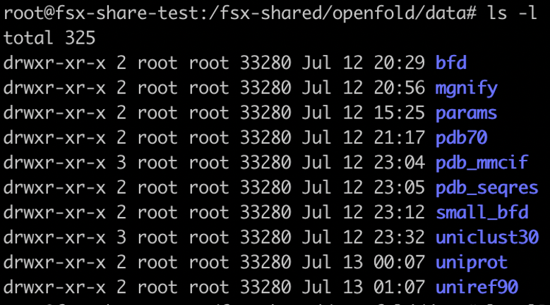
In this example, our shared FSx for Lustre folder is /fsx-shared, which got created after FSx for Lustre volume was mounted on the EKS cluster. When the job is complete, you should see the following folders in the fsx-shared folder.

Clone the OpenFold model files and download them into an S3 bucket and from there into an FSx for Lustre file system using the preceding steps. The following screenshot shows the seven files that should be in your FSX file system after you complete the download.

Create an OpenFold Docker file and .yaml manifest file

We have provided an OpenFold Docker file that you can use to build a base container that contains all the necessary dependencies to run OpenFold. To run OpenFold inference with pre-trained OpenFold models, you need to run the following code:

./run-openfold-inference/build.sh
./run-openfold-inference/push.sh
kubectl apply -f run-openfold-inference.yaml

The run_pretrained_openfold.py code provided in the OpenFold GitHub repo is an end-to-end inference code that takes in user inputs and computes alignments if needed using jackhmmer and hhsuite  binaries, loads the OpenFold model, and runs inference. It also includes other functionalities, including protein relaxation, model tracing, and multi-model, to name a few. Run the run_pretrained_openfold.py code in a Kubernetes pod using the .yaml file as follows:

apiVersion: v1
kind: Pod
metadata:
  name: openfold-inference-pod
spec:
  containers:
    - name: openfold-inference-worker
      image: <Path-to-ECR>
      imagePullPolicy: Always

      args:
        - "/fsx-shared/openfold/fasta_dir"
        - "/fsx-shared/openfold/data/pdb_mmcif/mmcif_files/"
        - "--config_preset=model_1_ptm"
        - "--uniref90_database_path=/fsx-shared/openfold/data/uniref90/uniref90.fasta"
        - "--mgnify_database_path=/fsx-shared/openfold/data/mgnify/mgy_clusters_2018_12.fa"
        - "--pdb70_database_path=/fsx-shared/openfold/data/pdb70/pdb70"
        - "--uniclust30_database_path=/fsx-shared/openfold/data/uniclust30/uniclust30_2018_08/uniclust30_2018_08"
        - "--output_dir=/fsx-shared/openfold/output_dir/"
        - "--bfd_database_path=/fsx-shared/openfold/data/bfd/bfd_metaclust_clu_complete_id30_c90_final_seq.sorted_opt"
        - "--model_device=cuda:0"
        - "--jackhmmer_binary_path=/opt/conda/envs/openfold_venv/bin/jackhmmer"
        - "--hhblits_binary_path=/opt/conda/envs/openfold_venv/bin/hhblits"
        - "--hhsearch_binary_path=/opt/conda/envs/openfold_venv/bin/hhsearch"
        - "--kalign_binary_path=/opt/conda/envs/openfold_venv/bin/kalign"
        - "--openfold_checkpoint_path=/fsx-shared/openfold/openfold_params/finetuning_ptm_2.pt"
      volumeMounts:
        - name: fsx-pv
          mountPath: /fsx-shared
        # The following enables the worker pods to use increased shared memory
        # which is required when specifying more than 0 data loader workers
        - name: dshm
          mountPath: /dev/shm
  volumes:
    - name: fsx-pv
      persistentVolumeClaim:
        claimName: fsx-pvc
    - name: dshm
      emptyDir:
        medium: Memory

Deploy OpenFold models as services and test the solution

To deploy OpenFold model servers as APIs, you need to complete the following steps:

1. Update inference_config.properties with information such as OpenFold model name, path to alignment directory, number of models to be deployed per server, model server instance type, number of servers, and server port.
2. Build the Docker image with build.sh.
3. Push the Docker image with push.sh.
4. Deploy the models with deploy.sh.

If you need to customize the OpenFold APIs, use the fastapi-server.py file, which has all the critical functionality needed to load OpenFold models, compute MSAs, and run inference.

Initialize the model_config, template_featurizer, data_processor, and feature_processor pipelines in fastapi-server.py by calling their respective classes. The precompute_alignment API takes in a protein tag and sequence as optional parameters and generates an alignment if one doesn’t already exist. The alignment_dir variable specifies the location where all the alignments are saved. The precompute_alignment API creates local alignment directories using the tags of each protein sequence. For this reason, make sure tags of each protein are unique. When the API is done running, the bfd_uniclust_hits.a3m, mgnify_hits.a3m, pdb70_hits.hhr, and uniref90_hits.a3m files are created in the local alignment directory.

Call the openfold_predictions inference API, which takes in a protein tag, sequence, and model ID. After the local alignment directory is identified, a processed feature dictionary is created, which gives an input batch. Next, a forward inference call is run with the model to give the output, which must be postprocessed with the prep_output function to yield an unrelaxed protein.

When the fastapi-server.py code is run, it loads multiple OpenFold models on each GPU across multiple instances. To keep track of which model is being loaded on each GPU, we need a global model dictionary that stores the model IDs of each model. You need to specify which checkpoint file you want to use and the number of models to be loaded per GPU, and those models are loaded when the container is run, as shown in the following code:

conda run --no-capture-output -n openfold_venv hypercorn fastapi-server:app -b 0.0.0.0:8080

The inference_config.properties file has inputs that you need to fill, including which checkpoint file to use, instance type for inference, number of model servers, and number of models to be loaded per server. In addition, it includes other inputs corresponding to input arguments in the run_pretrained_openfold.py code, such as number of CPUs, config_preset, and more. If you need to add additional functionality, such as addition protein relaxation, you can add relevant parameters in the inference_config.properties and make relevant changes in the fastapi-server.py code. If you specify models to be run on GPUs and, for example, two model servers with two models to be deployed per server, four Kubernetes applications are deployed (see below).

It’s important to specify the default namespace, otherwise there might be complications accessing FSx for Lustre shared volumes from compute resources in a custom namespace environment.

The deploy folder provides the template .yaml manifest file to deploy the OpenFold model as a service and a generate-yaml.sh shell script that creates a .yaml file for each service in a specific folder. For example, if you specify two model servers and p3.2xlarge instance type, openfold-gpu-0.yaml and openfold-gpu-1.yaml files are created in the app-openfold-gpu-p3.2xlarge folder. Then you can deploy the model services as follows:

kubectl apply -f app-openfold-gpu-p3.2xlarge

After the services are deployed, you can view the deployed services, as shown in the following screenshot.

Run alignment computation

Exposing alignment computation functionality as an API might have some specific use cases, but we need to be able to optimally use the EKS cluster so that alignment computation can be done in a parallel manner. We don’t need expensive GPU-based instances for alignment computation, so we need to add memory- or compute-intensive instances with a large number of CPUs. After we create an EKS cluster, we can create a new node group by running the eks-nodegroup-create.sh script, and we can scale the instances from the auto scaling group on the Amazon EC2 console after we make sure that the instances are in the same Availability Zone as FSx for Lustre. Because alignment computation is more memory intensive, we added r6 instances in the EKS cluster.

The cameo folder contains all the relevant scripts (Docker file; Python code; build, push, and shell scripts; and .yaml manifest file) that showcase how to run compute alignment on a FASTA file of protein sequences. To run alignment computation on your custom FASTA dataset, complete the following steps:

1. Save the FASTA file in the FSx folder.
2. Create one temporary FASTA file for each protein sequence and save it in the FSx folder.For the Cameo dataset, this is done by running kubectl apply -f temp-fasta.yaml in the cameo-fastas folder.
3. Update the alignment_dir path in the precompute_alignments.py code, which specifies the destination folder to save the alignments.
4. Build and push the Docker image to Amazon Elastic Container Registry (Amazon ECR).
5. Update the run-cameo.yaml file with the instance type and path to the Docker image in Amazon ECR and the number of CPUs if needed.
6. Update run-grid.py with the paths from steps 1 and 2. This code takes in the run-cameo.yaml file as a template, creates one .yaml file for each alignment computation job, and saves them in the cameo-yamls folder.
7. Finally, submit all the jobs by running kubectl apply -f cameo-yamls.

The precompute_alignments.py code loads a FASTA file of protein sequences. The run-cameo.yaml file shown in the following code just needs to specify the instance type, shared volume mount specification, and arguments such as number of CPUs for alignment computation:

kind: Pod
apiVersion: v1
metadata:
  name: cameo-pod

spec:
  nodeSelector:
    beta.kubernetes.io/instance-type: "r6i.xlarge"
  containers:
  - name: main
    image: <Path-to-ECR>
    imagePullPolicy: Always
    resources:
      requests:
        memory: "16Gi"
      limits:
        memory: "32Gi"
    args:
        - "--cpus=4"
        - "--one_file_path="
    volumeMounts:
    - name: fsx-pv
      mountPath: /fsx-shared
    - name: dshm
      mountPath: /dev/shm
  volumes:
  - name: fsx-pv
    persistentVolumeClaim:
      claimName: fsx-pvc
  - name: dshm
    emptyDir:
      medium: Memory

Depending on the availability of the compute nodes in the cluster, you could submit multiple Kubernetes jobs in parallel. Depending on your needs, you could have one or more dedicated CPU-based instances. After you create a CPU instance type node group, you can easily scale it up or down manually from the Amazon EC2 console. If the need arises for automatic cluster scaling, that could also be possible with the aws-do-eks framework, but would be included in a later iteration of this solution.

Performance tests

We have tested the performance of our architecture on the open-source Cameo dataset. This dataset has a total of 92 proteins of varying lengths. The following plot shows a histogram of the sequence lengths, which has a median sequence length of 236 and four sequences greater than 600.

We generated this plot with the following code:

import re
import matplotlib.pyplot as plt
import numpy as np

def parse_fasta(data):
    data = re.sub('>$', '', data, flags=re.M)
    lines = [
        l.replace('n', '')
        for prot in data.split('>') for l in prot.strip().split('n', 1)
    ][1:]
    tags, seqs = lines[::2], lines[1::2]

    tags = [t.split()[0]+'_'+t.split()[6] for t in tags]

    return tags, seqs

test_squences_path = './Cameo/cameo_protein_targets.fasta'

# Gather input sequences
with open(test_squences_path, "r") as fp:
    data = fp.read()

tags, seqs = parse_fasta(data)

all_lens = []
for (tag,seq) in zip(tags,seqs):
    all_lens.append(len(seq))

plt.hist(all_lens, density=True, bins=50)  # density=False would make counts
plt.ylabel('Probability')
plt.xlabel('Sequence Length');

The alignment computation is memory intensive and not compute intensive, which means that using memory optimized instances will be more cost performant than compute optimized instances. For our tests, we selected the r6i.xlarge instances, which have 4 vCPUs and a 32 GB of memory, and one pod was spun off for one alignment computation job for each protein sequence.

The following table shows the results for the alignment computation jobs. We see that with 92 r6i.xlarge instances, we could complete alignment computation for 92 proteins for under $60. For reference, we compared 1 c6i.12xlarge instance with just one pod that took over 2 days to finish computation.

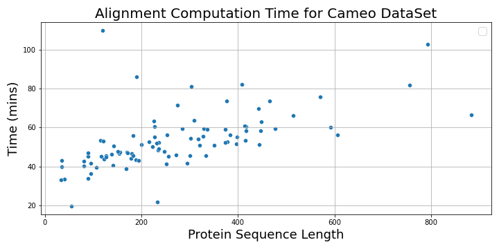
The following plot shows the alignment computation time vs. protein sequence lengths.

The following plots show max CPU utilization of the 92×4 = 368 vCPUs in the r6i.xlarge auto-scaling group. The bottom plot is just a continuation of the top one. We see that the CPUs were utilized for their maximum capacity and gradually go down to 0 when all jobs finish.

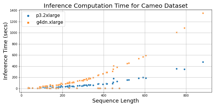
Finally, after the MSAs are computed, we can run the inference by calling the model server APIs. The following table shows the total inference times on the Cameo dataset for p3.2xlarge vs g4dn.xlarge instances. With p3.2xlarge machine, MSA computation over 92 proteins of the Cameo dataset can be done three times faster than g4dn.xlarge machine.

The following plot shows the total time taken to load the MSA files and perform inference on a p3.2xlarge instance and a g4dn.xlarge instance as a function of protein sequence length. For sequences longer than 200, the inference time with p3.2xlarge instance is three times faster than g4dn.xlarge instance, whereas for shorter sequences, it’s 1–2 times faster.

Clean up

It’s important to spin down resources after model training in order to avoid costs associated with running idle instances. With each script that creates resources, the GitHub repo provides a matching script to delete them. To clean up our setup, we must delete the FSx file system before deleting the cluster, because it’s associated with a subnet in the cluster’s VPC. To delete the FSx file system, run the following command from inside the fsx folder:

kubectl delete -f fsx-pvc-dynamic.yaml
./delete.sh

Note that this will not only delete the persistent volume, it will also delete the FSx file system, and all the data on the file system will be lost.

When this step is complete, we can delete the cluster by using the following script in the eks folder:

./eks-delete.sh

This will delete all the existing pods, remove the cluster, and delete the VPC created in the beginning.

Conclusion

In this post, we showed how to use an EKS cluster to run inference with OpenFold models. We have published the instructions on the AWS EKS Architecture For OpenFold Inference GitHub repo, where you can find step-by-step instructions on how to create an EKS cluster, mount a shared file system to it, download OpenFold data, perform MSA computation, and deploy OpenFold models as APIs. For more information on OpenFold, visit the OpenFold GitHub repo.

About the authors

Shubha Kumbadakone is a Sr. GTM Specialist for self-managed machine learning with a focus on open-source software and tools. She has more than 17 years of experience in cloud infrastructure and machine learning and is helping customers build their distributed training and inference at scale for their ML models on AWS. She also holds a patent on a caching algorithm for rapid resume from hibernation for mobile systems.

Ankur Srivastava is a Sr. Solutions Architect in the ML Frameworks Team. He focuses on helping customers with self-managed distributed training and inference at scale on AWS. His experience includes industrial predictive maintenance, digital twins, probabilistic design optimization and has completed his doctoral studies from Mechanical Engineering at Rice University and post-doctoral research from Massachusetts Institute of Technology.

Sachin Kadyan is a leading developer of OpenFold.

Read More

This post walks you through a few new features that make it simple to design a conversational flow entirely within Amazon Lex that adheres to best practices for IVR design related to retry prompting. We also cover how to configure a DTMF-only prompt as well as other attributes like timeouts and barge-in.

When designing an IVR solution, it’s best practice to provide an initial prompt that is short and to the point in order to allow a customer to get through the voice interaction quickly. If the system doesn’t understand, it needs to provide a more detailed prompt to guide the user to provide the required information. Should that fail, it’s best practice to fall back to DTMF, and ask the caller to enter the information using their dial pad.

Sometimes, we may also want to define a slot value as voice or DTMF only in order to provide more control over how the system accepts input.

Amazon Lex now lets you set session attributes to control voice and DTMF input modes. You can control voice and DTMF configuration for each slot separately for the initial prompt and each retry prompt using the new advance retry settings. There is also a new setting: Play the messages in order. This sets the message variations for a slot to play in the order they have been entered instead of randomly.

Solution overview

The following short video provides an overview of the concepts covered in this post.

To demonstrate these new features, we deploy a new Amazon Lex bot starting with the BookTrip example bot. We modify the configurations for capturing the CheckinDate slot value. We then integrate the bot into an Amazon Connect contact flow for testing.

Prerequisites

To implement this solution, you need the following prerequisites:

• An AWS account with permission to create Amazon Lex bots
• An Amazon Connect instance and permissions to create new contact flows and add new Amazon Lex bots

Create an Amazon Lex bot

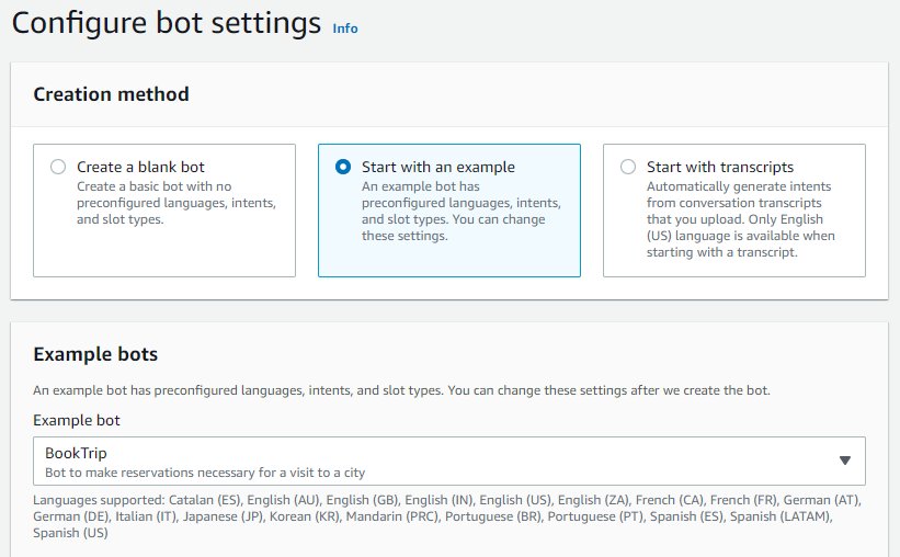
To start building your bot, complete the following steps:

1. On the Amazon Lex console, choose Bots in the navigation pane.
2. Choose Create bot.
3. For Creation method, select Start with an example.
4. For Example bot, choose BookTrip.
   
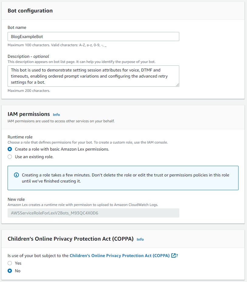
5. For Bot name, enter a name.
6. For Description, enter an optional description.
7. For IAM permissions¸ select Create a role with basic Amazon Lex permissions.
8. For Children’s Online Privacy Protection Act, select No.
   
9. Choose Next.
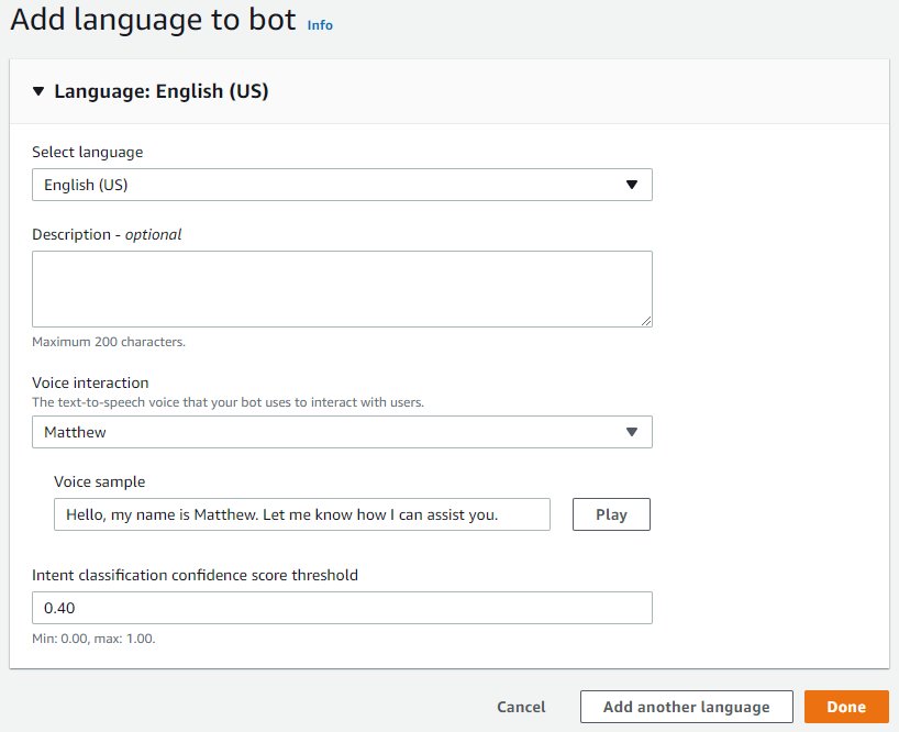
10. For Voice interaction, choose a voice (for this post, we choose Matthew).
11. Choose Done to create the bot.
    
    You can now see the page with the details for the BookHotel intent.
    
12. Choose Save intent and then choose Visual builder to get a better overview of the conversational design of this intent.You’re presented with a drag and drop editor where you can easily see the progression of the conversation as slots are collected to fulfill the BookHotel intent.
    
13. Choose the edit icon for the CheckInDate block.
    
14. Choose the gear icon next to Slot prompt.
    
    This opens up additional options for your slot prompts.
15. Select Play the messages in order.
    This sets the prompt variations we’re about to configure to be played in the order they have been defined. This is very useful because it allows us to specify different prompts for the initial utterance and our first and second retry.
    
    Now you can specify the prompts to use when eliciting this slot.
16. Add two more variations to be used as the first and second retry prompt:
    1. “What day do you want to check in? You can say things like tomorrow, Next Sunday, or November 13th.”
    2. “Please enter the day you want to check in using four-digit year, two-digit-month, and two-digit day.”
       
17. Choose Configure advanced retry settings.
    Here you can configure the number of retries, if audio or DTMF should be enabled for each retry, as well as configurations for timeouts and the characters to use for Deletion and End when using DTMF.
18. Leave these settings unchanged and choose Confirm.
    
19. Choose Save intent and then choose Build to build the bot.

Integrate the bot with an Amazon Connect contact flow

You can use an existing Amazon Connect instance, or create a new instance. To integrate the Amazon Lex bot, complete the following steps:

1. Add the bot to your Amazon Connect instance to allow you to use it in contact flows.
2. Create a new contact flow.
3. Add a Get customer input block.
   The Play prompt block is optional.
   
4. Add a greeting prompt to be played using text-to-speech. For example, “Welcome to Octank travel and hospitality. How can we help you today?”
5. Select the Amazon Lex bot that we created earlier.
6. For Alias, choose TestBotAlias.
   You should only use the TestBotAlias alias for testing; Amazon Lex V2 limits the number of runtime requests that you can make to the alias.If the bot doesn’t appear on the drop-down menu, you haven’t added it properly to your instance of Amazon Connect. Go back and review that step in the instructions.
   
7. Claim a new phone number or use an existing one and point it to the new contact flow.
8. Call in and test the bot:

Welcome to Octank travel and hospitality. How can we help you today?
I want to book a hotel.

What city will you be staying in?
New York

What day do you want to check in?
Hedgehog. (You can say anything here that is not interpreted as a date.)

What day do you want to check in? You can say things like tomorrow, Next Sunday, or November 13th.
Hedgehog.

Please enter the day you want to check in using four-digit year, two-digit-month, and two-digit day.
Sunday. (This will be transformed to the corresponding date. Even though the prompt asked for DTMF, voice is still enabled. If you want to disable voice for this specific retry attempt, this can be done in the advanced retry settings of the bot.)

How many nights will you be staying?
Four.

What type of room would you like, queen, king, or deluxe?
King.

Okay, I have you down for a four-night stay in New York starting {CheckInDate}. Shall I book the reservation?
Yes

Notice how the three slot prompts were played in order.

Add session attributes

You can now add session attributes that are sent to the Amazon Lex bot.

1. Add the Get customer input block and add the following attribute under Session attributes.
2. Set x-amz-lex:allow-audio-input:BookHotel:CheckInDate to False.
   
3. Save and publish the contact flow and call in again.Notice how you can’t speak a date when asked for a check-in date. Entering the date using DTMF (2022 11 22) will still work.
4. Set x-amz-lex:allow-audio-input:BookHotel:CheckInDate to True (or just remove it, since the bot is configured to allow voice per default) and set x-amz-lex:allow-interrupt:*:* to False.
   
5. Save and publish the contact flow.

You’re now able to speak the date, but you can’t interrupt the prompt that is asking for the date.

For a list of these and other attributes that you can use to disable DTMF input or modify the timeouts for voice and DTMF, refer to Configuring timeouts for capturing user input.

You can also set session attributes in the Get customer input block using external or user-defined attributes. This makes it possible to store the configuration for your Amazon Lex bots externally, and fetch them using an AWS Lambda function. You can also update these attributes based on business rules. This would, for example, allow you to let a customer opt-in to setting all interactions to DTMF only if they’re calling from a noisy environment.

Clean up

When you’re done using this solution, delete the Amazon Lex bot and release the phone number if you claimed a new one.

Conclusion

These recently released features make it easier to design a conversational flow entirely within Amazon Lex that adheres to best practices for IVR design related to retry prompts. These new attributes also make it possible to define the behavior of an Amazon Lex bot through configuration, allowing changes to be made without updating and redeploying contact flows.

Try out these new features to see how they can provide a better customer experience in your contact center!

About the author

Thomas Rindfuss is a Sr. Solutions Architect on the Amazon Lex team. He invents, develops, prototypes, and evangelizes new technical features and solutions for Language AI services that improves the customer experience and eases adoption.

Read More

As AI adoption is accelerating across the industry, customers are building sophisticated models that take advantage of new scientific breakthroughs in deep learning. These next-generation models allow you to achieve state-of-the-art, human-like performance in the fields of natural language processing (NLP), computer vision, speech recognition, medical research, cybersecurity, protein structure prediction, and many others. For instance, large language models like GPT-3, OPT, and BLOOM can translate, summarize, and write text with human-like nuances. In the computer vision space, text-to-image diffusion models like DALL-E and Imagen can create photorealistic images from natural language with a higher level of visual and language understanding from the world around us. These multi-modal models provide richer features for various downstream tasks and the ability to fine-tune them for specific domains, and they bring powerful business opportunities to our customers.

These deep learning models keep growing in terms of size, and typically contain billions of model parameters to scale model performance for a wide variety of tasks, such as image generation, text summarization, language translation, and more. There is also a need to customize these models to deliver a hyper-personalized experience to individuals. As a result, a greater number of models are being developed by fine-tuning these models for various downstream tasks. To meet the latency and throughput goals of AI applications, GPU instances are preferred over CPU instances (given the computational power GPUs offer). However, GPU instances are expensive and costs can add up if you’re deploying more than 10 models. Although these models can potentially bring impactful AI applications, it may be challenging to scale these deep learning models in cost-effective ways due to their size and number of models.

Amazon SageMaker multi-model endpoints (MMEs) provide a scalable and cost-effective way to deploy a large number of deep learning models. MMEs are a popular hosting choice to host hundreds of CPU-based models among customers like Zendesk, Veeva, and AT&T. Previously, you had limited options to deploy hundreds of deep learning models that needed accelerated compute with GPUs. Today, we announce MME support for GPU. Now you can deploy thousands of deep learning models behind one SageMaker endpoint. MMEs can now run multiple models on a GPU core, share GPU instances behind an endpoint across multiple models, and dynamically load and unload models based on the incoming traffic. With this, you can significantly save cost and achieve the best price performance.

In this post, we show how to run multiple deep learning models on GPU with SageMaker MMEs.

SageMaker MMEs

SageMaker MMEs enable you to deploy multiple models behind a single inference endpoint that may contain one or more instances. With MMEs, each instance is managed to load and serve multiple models. MMEs enable you to break the linearly increasing cost of hosting multiple models and reuse infrastructure across all the models.

The following diagram illustrates the architecture of a SageMaker MME.

The SageMaker MME dynamically downloads models from Amazon Simple Storage Service (Amazon S3) when invoked, instead of downloading all the models when the endpoint is first created. As a result, an initial invocation to a model might see higher inference latency than the subsequent inferences, which are completed with low latency. If the model is already loaded on the container when invoked, then the download and load step is skipped and the model returns the inferences with low latency. For example, assume you have a model that is only used a few times a day. It is automatically loaded on demand, whereas frequently accessed models are retained in memory and invoked with consistently low latency.

SageMaker MMEs with GPU support

SageMaker MMEs with GPU work using NVIDIA Triton Inference Server. NVIDIA Triton Inference Server is an open-source inference serving software that simplifies the inference serving process and provides high inference performance. Triton supports all major training and inference frameworks, such as TensorFlow, NVIDIA® TensorRT, PyTorch, MXNet, Python, ONNX, XGBoost, Scikit-learn, RandomForest, OpenVINO, custom C++, and more. It offers dynamic batching, concurrent runs, post-training quantization, and optimal model configuration to achieve high-performance inference. Additionally, NVIDIA Triton Inference Server has been extended to implement MME API contract, to integrate with MME.

The following diagram illustrates an MME workflow.

The workflow steps are as follows:

1. The SageMaker MME receives an HTTP invocation request for a particular model using TargetModel in the request along with the payload.
2. SageMaker routes traffic to the right instance behind the endpoint where the target model is loaded. SageMaker understands the traffic pattern across all the models behind the MME and smartly routes requests.
3. SageMaker takes care of model management behind the endpoint, dynamically loads the model to the container’s memory, and unloads the model based from the shared fleet of GPU instances to give the best price performance.
4. SageMaker dynamically downloads models from Amazon S3 to the instance’s storage volume. If the invoked model isn’t available on the instance storage volume, the model is downloaded onto the instance storage volume. If the instance storage volume reaches capacity, SageMaker deletes any unused models from the storage volume.
5. SageMaker loads the model to the NVIDIA Triton container’s memory on a GPU accelerated instance and serve the inference request. The GPU core is shared by all the models in an instance. If the model is already loaded in the container memory, the subsequent requests are served faster because SageMaker doesn’t need to download and load it again.
6. SageMaker takes care of traffic shaping to the MME endpoint and maintains optimal model copies on GPU instances for best price performance. It continues to route traffic to the instance where the model is loaded. If the instance resources reach capacity due to high utilization, SageMaker unloads the least-used models from the container to free up resources to load more frequently used models.

SageMaker MMEs can horizontally scale using an auto scaling policy, and provision additional GPU compute instances based on metrics such as invocations per instance and GPU utilization to serve any traffic surge to MME endpoints.

Solution overview

In this post, we show you how to use the new features of SageMaker MMEs with GPU with a computer vision use case. For demonstration purposes, we use a ResNet-50 convolutional neural network pre-trained model that can classify images into 1,000 categories. We discuss how to do the following:

• Use an NVIDIA Triton inference container on SageMaker MMEs, using different Triton model framework backends such and PyTorch and TensorRT
• Convert ResNet-50 models to optimized TensorRT engine format and deploy it with a SageMaker MME
• Set up auto scaling policies for the MME
• Get insights into instance and invocation metrics using Amazon CloudWatch

Create model artifacts

This section walks through the steps to prepare a ResNet-50 pre-trained model to be deployed on an SageMaker MME using Triton Inference Server model configurations. You can reproduce all the steps using the step-by-step notebook on GitHub.

For this post, we demonstrate deployment with two models. However, you can prepare and deploy hundreds of models. The models may or may not share the same framework.

Prepare a PyTorch model

First, we load a pre-trained ResNet50 model using the torchvision models package. We save the model as a model.pt file in TorchScript optimized and serialized format. TorchScript compiles a forward pass of the ResNet50 model in eager mode with example inputs, so we pass one instance of an RGB image with three color channels of dimension 224 x 224.

Then we need to prepare the models for Triton Inference Server. The following code shows the model repository for the PyTorch framework backend. Triton uses the model.pt file placed in the model repository to serve predictions.

resnet
├── 1
│   └── model.pt
└── config.pbtxt

The model configuration file config.pbtxt must specify the name of the model (resnet), the platform and backend properties (pytorch_libtorch), max_batch_size (128), and the input and output tensors along with the data type (TYPE_FP32) information. Additionally, you can specify instance_group and dynamic_batching properties to achieve high performance inference. See the following code:

name: "resnet"
platform: "pytorch_libtorch"
max_batch_size: 128
input {
  name: "INPUT__0"
  data_type: TYPE_FP32
  dims: 3
  dims: 224
  dims: 224
}
output {
  name: "OUTPUT__0"
  data_type: TYPE_FP32
  dims: 1000
}

Prepare the TensorRT model

NVIDIA TensorRT is an SDK for high-performance deep learning inference, and includes a deep learning inference optimizer and runtime that delivers low latency and high throughput for inference applications. We use the command line tool trtexec to generate a TensorRT serialized engine from an ONNX model format. Complete the following steps to convert a ResNet-50 pre-trained model to NVIDIA TensorRT:

1. Export the pre-trained ResNet-50 model into an ONNX format using torch.onnx.This step runs the model one time to trace its run with a sample input and then exports the traced model to the specified file model.onnx.
2. Use trtexec to create a TensorRT engine plan from the model.onnx file. You can optionally reduce the precision of floating-point computations, either by simply running them in 16-bit floating point, or by quantizing floating point values so that calculations can be performed using 8-bit integers.

The following code shows the model repository structure for the TensorRT model:

resnet
├── 1
│   └── model.plan
└── config.pbtxt

For the TensorRT model, we specify tensorrt_plan as the platform and input the Tensor specifications of the image of dimension 224 x 224, which has the color channels. The output Tensor with 1,000 dimensions is of type TYPE_FP32, corresponding to the different object categories. See the following code:

name: "resnet"
platform: "tensorrt_plan"
max_batch_size: 128
input {
  name: "input"
  data_type: TYPE_FP32
  dims: 3
  dims: 224
  dims: 224
}
output {
  name: "output"
  data_type: TYPE_FP32
  dims: 1000
}
model_warmup {
    name: "bs128 Warmup"
    batch_size: 128
    inputs: {
        key: "input"
        value: {
            data_type: TYPE_FP32
            dims: 3
            dims: 224
            dims: 224
            zero_data: false
        }
    }
}

Store model artifacts in Amazon S3

SageMaker expects the model artifacts in .tar.gz format. They should also satisfy Triton container requirements such as model name, version, config.pbtxt files, and more. tar the folder containing the model file as .tar.gz and upload it to Amazon S3:

!mkdir -p triton-serve-pt/resnet/1/
!mv -f workspace/model.pt triton-serve-pt/resnet/1/
!tar -C triton-serve-pt/ -czf resnet_pt_v0.tar.gz resnet
model_uri_pt = sagemaker_session.upload_data(path="resnet_pt_v0.tar.gz", key_prefix="resnet-mme-gpu")
!mkdir -p triton-serve-trt/resnet/1/
!mv -f workspace/model.plan triton-serve-trt/resnet/1/
!tar -C triton-serve-trt/ -czf resnet_trt_v0.tar.gz resnet
model_uri_trt = sagemaker_session.upload_data(path="resnet_trt_v0.tar.gz", key_prefix="resnet-mme-gpu")

Now that we have uploaded the model artifacts to Amazon S3, we can create a SageMaker MME.

Deploy models with an MME

We now deploy a ResNet-50 model with two different framework backends (PyTorch and TensorRT) to a SageMaker MME.

Note that you can deploy hundreds of models, and the models can use the same framework. They can also use different frameworks, as shown in this post.

We use the AWS SDK for Python (Boto3) APIs create_model, create_endpoint_config, and create_endpoint to create an MME.

Define the serving container

In the container definition, define the model_data_url to specify the S3 directory that contains all the models that the SageMaker MME uses to load and serve predictions. Set Mode to MultiModel to indicate that SageMaker creates the endpoint with MME container specifications. We set the container with an image that supports deploying MMEs with GPU. See the following code:

container = {
"Image": <IMAGE>,
"ModelDataUrl": <MODEL_DATA_URL>,
"Mode": "MultiModel"
}

Create a multi-model object

Use the SageMaker Boto3 client to create the model using the create_model API. We pass the container definition to the create model API along with ModelName and ExecutionRoleArn:

create_model_response = sm_client.create_model(
    ModelName=<MODEL_NAME>, ExecutionRoleArn=role, PrimaryContainer=container
)

Define MME configurations

Create MME configurations using the create_endpoint_config Boto3 API. Specify an accelerated GPU computing instance in InstanceType (we use the g4dn.4xlarge instance type). We recommend configuring your endpoints with at least two instances. This allows SageMaker to provide a highly available set of predictions across multiple Availability Zones for the models.

Based on our findings, you can get better price performance on ML-optimized instances with a single GPU core. Therefore, MME support for GPU feature is only enabled for single-GPU core instances. For a full list of instances supported, refer to Supported GPU Instance types.

create_endpoint_config_response = sm_client.create_endpoint_config(
    EndpointConfigName=<ENDPOINT_CONFIG_NAME>,
    ProductionVariants=[
        {
            "InstanceType": "ml.g4dn.4xlarge",
            "InitialVariantWeight": 1,
            "InitialInstanceCount": 2,
            "ModelName": <MODEL_NAME>,
            "VariantName": "AllTraffic",
        }
    ],
)

Create an MME

With the preceding endpoint configuration, we create a SageMaker MME using the create_endpoint API. SageMaker creates the MME, launches the ML compute instance g4dn.4xlarge, and deploys the PyTorch and TensorRT ResNet-50 models on them. See the following code:

create_endpoint_response = sm_client.create_endpoint(
    EndpointName=<ENDPOINT_NAME>, EndpointConfigName=<ENDPOINT_CONFIG_NAME>
)

Invoke the target model on the MME

After we create the endpoint, we can send an inference request to the MME using the invoke_enpoint API. We specify the TargetModel in the invocation call and pass in the payload for each model type. The following code is a sample invocation for the PyTorch model and TensorRT model:

runtime_sm_client.invoke_endpoint(
    EndpointName=<ENDPOINT_NAME>,
    ContentType="application/octet-stream",
    Body=json.dumps(pt_payload),
    TargetModel='resnet_pt_v0.tar.gz', #PyTorch Model
)
runtime_sm_client.invoke_endpoint(
    EndpointName=<ENDPOINT_NAME>, 
    ContentType="application/octet-stream", 
    Body=json.dumps(trt_payload),
    TargetModel='resnet_trt_v0.tar.gz' #TensorRT Model
)

Set up auto scaling policies for the GPU MME

SageMaker MMEs support automatic scaling for your hosted models. Auto scaling dynamically adjusts the number of instances provisioned for a model in response to changes in your workload. When the workload increases, auto scaling brings more instances online. When the workload decreases, auto scaling removes unnecessary instances so that you don’t pay for provisioned instances that you aren’t using.

In the following scaling policy, we use the custom metric GPUUtilization in the TargetTrackingScalingPolicyConfiguration configuration and set a TargetValue of 60.0 for the target value of that metric. This autoscaling policy provisions additional instances up to MaxCapacity when GPU utilization is more than 60%.

auto_scaling_client = boto3.client('application-autoscaling')

resource_id='endpoint/' + <ENDPOINT_NAME> + '/variant/' + 'AllTraffic' 
response = auto_scaling_client.register_scalable_target(
    ServiceNamespace='sagemaker',
    ResourceId=resource_id,
    ScalableDimension='sagemaker:variant:DesiredInstanceCount',
    MinCapacity=1,
    MaxCapacity=5
)

response = auto_scaling_client.put_scaling_policy(
    PolicyName='GPUUtil-ScalingPolicy',
    ServiceNamespace='sagemaker',
    ResourceId=resource_id,
    ScalableDimension='sagemaker:variant:DesiredInstanceCount', 
    PolicyType='TargetTrackingScaling',
    TargetTrackingScalingPolicyConfiguration={
        'TargetValue': 60.0, 
        'CustomizedMetricSpecification':
        {
            'MetricName': 'GPUUtilization',
            'Namespace': '/aws/sagemaker/Endpoints',
            'Dimensions': [
                {'Name': 'EndpointName', 'Value': <ENDPOINT_NAME> },
                {'Name': 'VariantName','Value': 'AllTraffic'}
            ],
            'Statistic': 'Average',
            'Unit': 'Percent'
        },
        'ScaleInCooldown': 600,
        'ScaleOutCooldown': 200 
    }
)

We recommend using GPUUtilization or InvocationsPerInstance to configure auto scaling policies for your MME. For more details, see Set Autoscaling Policies for Multi-Model Endpoint Deployments

CloudWatch metrics for GPU MMEs

SageMaker MMEs provide the following instance-level metrics to monitor:

• LoadedModelCount – Number of models loaded in the containers
• GPUUtilization – Percentage of GPU units that are used by the containers
• GPUMemoryUtilization – Percentage of GPU memory used by the containers
• DiskUtilization – Percentage of disk space used by the containers

These metrics allow you to plan for effective utilization of GPU instance resources. In the following graph, we see GPUMemoryUtilization was 38.3% when more than 16 ResNet-50 models were loaded in the container. The sum of each individual CPU core’s utilization (CPUUtilization) was 60.9%, and percentage of memory used by the containers (MemoryUtilization) was 9.36%.

SageMaker MMEs also provide model loading metrics to get model invocation-level insights:

• ModelLoadingWaitTime – Time interval for the model to be downloaded or loaded
• ModelUnloadingTime – Time interval to unload the model from the container
• ModelDownloadingTime – Time to download the model from Amazon S3
• ModelCacheHit – Number of invocations to the model that are already loaded onto the container

In the following graph, we can observe that it took 8.22 seconds for a model to respond to an inference request (ModelLatency), and 24.1 milliseconds was added to end-to-end latency due to SageMaker overheads (OverheadLatency). We can also see any errors metrics from calls to invoke an endpoint API call, such as Invocation4XXErrors and Invocation5XXErrors.

For more information about MME CloudWatch metrics, refer to CloudWatch Metrics for Multi-Model Endpoint Deployments.

Summary

In this post, you learned about the new SageMaker multi-model support for GPU, which enables you to cost-effectively host hundreds of deep learning models on accelerated compute hardware. You learned how to use the NVIDIA Triton Inference Server, which creates a model repository configuration for different framework backends, and how to deploy an MME with auto scaling. This feature will allow you to scale hundreds of hyper-personalized models that are fine-tuned to cater to unique end-user experiences in AI applications. You can also leverage this feature to achieve needful price performance for your inference application using fractional GPUs.

To get started with MME support for GPU, see Multi-model endpoint support for GPU.

About the authors

Dhawal Patel is a Principal Machine Learning Architect at AWS. He has worked with organizations ranging from large enterprises to mid-sized startups on problems related to distributed computing and artificial intelligence. He focuses on deep learning, including NLP and computer vision domains. He helps customers achieve high-performance model inference on Amazon SageMaker.

Vikram Elango is a Senior AI/ML Specialist Solutions Architect at Amazon Web Services, based in Virginia, US. Vikram helps global financial and insurance industry customers with design, implementation and thought leadership to build and deploy machine learning applications at scale. He is currently focused on natural language processing, responsible AI, inference optimization, and scaling ML across the enterprise. In his spare time, he enjoys traveling, hiking, cooking, and camping with his family.

Saurabh Trikande is a Senior Product Manager for Amazon SageMaker Inference. He is passionate about working with customers and is motivated by the goal of democratizing machine learning. He focuses on core challenges related to deploying complex ML applications, multi-tenant ML models, cost optimizations, and making deployment of deep learning models more accessible. In his spare time, Saurabh enjoys hiking, learning about innovative technologies, following TechCrunch, and spending time with his family.

Deepti Ragha is a Software Development Engineer in the Amazon SageMaker team. Her current work focuses on building features to host machine learning models efficiently. In her spare time, she enjoys traveling, hiking and growing plants.

Nikhil Kulkarni is a software developer with AWS Machine Learning, focusing on making machine learning workloads more performant on the cloud and is a co-creator of AWS Deep Learning Containers for training and inference. He’s passionate about distributed Deep Learning Systems. Outside of work, he enjoys reading books, fiddling with the guitar, and making pizza.

Jiahong Liu is a Solution Architect on the Cloud Service Provider team at NVIDIA. He assists clients in adopting machine learning and AI solutions that leverage NVIDIA accelerated computing to address their training and inference challenges. In his leisure time, he enjoys origami, DIY projects, and playing basketball.

Eliuth Triana is a Developer Relations Manager on the NVIDIA-AWS team. He connects Amazon and AWS product leaders, developers, and scientists with NVIDIA technologists and product leaders to accelerate Amazon ML/DL workloads, EC2 products, and AWS AI services. In addition, Eliuth is a passionate mountain biker, skier, and poker player.

Read More