Vice president of ML and AI Services says more than 100,000 customers are doing machine learning on AWS.Read More
Amazon SageMaker’s fifth birthday: Looking back, looking forward
Vice president Bratin Saha reflects on the past and future of Amazon Web Services’ machine learning tools and AI services.Read More
Women in Machine Learning Symposium 2022 – Event Recap

Posted by Joana Carrasqueira, Developer Relations Program Manager
Thank you to everyone who joined us at the second Women in Machine Learning Symposium!
Last year we founded the Women in Machine Learning program, with the goal of building an inclusive space for all intersections of diversity and to give a voice and platform to women passionate about ML. Hundreds joined to share tips and insights for careers in ML, learned how to get involved in the community, contributed to open source, and much more.
This year, thousands of ML practitioners joined from all over the world. Everyone came together to learn the latest Machine Learning tools and techniques, get the scoop on the newest ML products from Google, and learn directly from several amazing women in the field.
During the keynote we announced:
- Simple ML for Sheets – Simple ML is an add-on, in beta, for Google Sheets from the TensorFlow team that helps make machine learning accessible to all. Anyone, even people without programming or ML expertise, can experiment and apply some of the power of machine learning to their data in Google Sheets with just a few clicks. Watch the demo here.
- MediaPipe Previews – We invited developers to preview low-code APIs that provide solutions to common on-device ML challenges across vision, natural language and audio. We also opened MediaPipe Studio, a web-based interface that provides a new way to prototype and benchmark ML solutions.
- TensorFlow Recommendation Systems Hub – We published a new dedicated page on TensorFlow.org where developers can find tools and guidance for building world-class recommendation systems with the TensorFlow ecosystem.
- Upcoming Sign Language AI Kaggle Competition – Our first Sign Language AI Competition to help the partners of deaf children learn to sign launches soon. Sign up to get notified when it launches.
Following is a quick recap, and workshops from the event. Thanks again.
Workshops:
Introduction to Machine Learning
TensorFlow Lite in Android with Google Play Services
Advanced On-Device ML Made Easy with MediaPipe
Generative Adversarial Networks (GANs) and Stable Diffusion
What’s Next?
Subscribe to the TensorFlow channel on YouTube and check out the Women in Machine Learning Symposium 2022 playlist at your convenience!
Economics students in Africa build computational skills
Amazon provided funding for two-week workshop led by Nobel Prize winner Thomas Sargent.Read More
How Amazon Robotics is working to eliminate the need for barcodes
Why multimodal identification is a crucial step in automating item identification at Amazon scale.Read More
Efficient Multi-Objective Neural Architecture Search with Ax
Multi-Objective Optimization in Ax enables efficient exploration of tradeoffs (e.g. between model performance and model size or latency) in Neural Architecture Search.Read More
Prepare data from Amazon EMR for machine learning using Amazon SageMaker Data Wrangler
Data preparation is a principal component of machine learning (ML) pipelines. In fact, it is estimated that data professionals spend about 80 percent of their time on data preparation. In this intensive competitive market, teams want to analyze data and extract more meaningful insights quickly. Customers are adopting more efficient and visual ways to build data processing systems.
Amazon SageMaker Data Wrangler simplifies the data preparation and feature engineering process, reducing the time it takes from weeks to minutes by providing a single visual interface for data scientists to select, clean data, create features, and automate data preparation in ML workflows without writing any code. You can import data from multiple data sources, such as Amazon Simple Storage Service (Amazon S3), Amazon Athena, Amazon Redshift, and Snowflake. You can now also use Amazon EMR as a data source in Data Wrangler to easily prepare data for ML.
Analyzing, transforming, and preparing large amounts of data is a foundational step of any data science and ML workflow. Data professionals such as data scientists want to leverage the power of Apache Spark, Hive, and Presto running on Amazon EMR for fast data preparation, but the learning curve is steep. Our customers wanted the ability to connect to Amazon EMR to run ad hoc SQL queries on Hive or Presto to query data in the internal metastore or external metastore (e.g., AWS Glue Data Catalog), and prepare data within a few clicks.
This blog article will discuss how customers can now find and connect to existing Amazon EMR clusters using a visual experience in SageMaker Data Wrangler. They can visually inspect the database, tables, schema, and Presto queries to prepare for modeling or reporting. They can then quickly profile data using a visual interface to assess data quality, identify abnormalities or missing or erroneous data, and receive information and recommendations on how to address these issues. Additionally, they can analyze, clean, and engineer features with the aid of more than a dozen additional built-in analyses and 300+ extra built-in transformations backed by Spark without writing a single line of code.
Solution overview
Data professionals can quickly find and connect to existing EMR clusters using SageMaker Studio configurations. Additionally, data professionals can terminate EMR clusters with only a few clicks from SageMaker Studio using predefined templates and on-demand creation of EMR clusters. With the help of these tools, customers may jump right into the SageMaker Studio universal notebook and write code in Apache Spark, Hive, Presto, or PySpark to perform data preparation at scale. Due to a steep learning curve for creating Spark code to prepare data, not all data professionals are comfortable with this procedure. With Amazon EMR as a data source for Amazon SageMaker Data Wrangler, you can now quickly and easily connect to Amazon EMR without writing a single line of code.
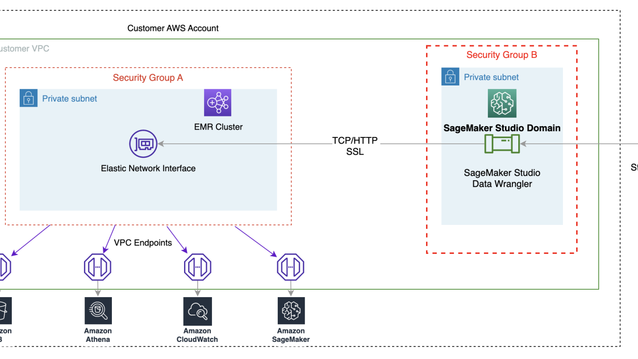
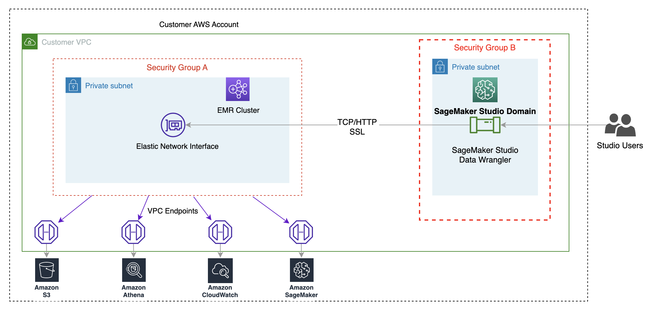
The following diagram represents the different components used in this solution.
We demonstrate two authentication options that can be used to establish a connection to the EMR cluster. For each option, we deploy a unique stack of AWS CloudFormation templates.
The CloudFormation template performs the following actions when each option is selected:
- Creates a Studio Domain in VPC-only mode, along with a user profile named
studio-user. - Creates building blocks, including the VPC, endpoints, subnets, security groups, EMR cluster, and other required resources to successfully run the examples.
- For the EMR cluster, connects the AWS Glue Data Catalog as metastore for EMR Hive and Presto, creates a Hive table in EMR, and fills it with data from a US airport dataset.
- For the LDAP CloudFormation template, creates an Amazon Elastic Compute Cloud (Amazon EC2) instance to host the LDAP server to authenticate the Hive and Presto LDAP user.
Option 1: Lightweight Access Directory Protocol
For the LDAP authentication CloudFormation template, we provision an Amazon EC2 instance with an LDAP server and configure the EMR cluster to use this server for authentication. This is TLS Enabled.
Option 2: No-Auth
In the No-Auth authentication CloudFormation template, we use a standard EMR cluster with no authentication enabled.
Deploy the resources with AWS CloudFormation
Complete the following steps to deploy the environment:
- Sign in to the AWS Management Console as an AWS Identity and Access Management (IAM) user, preferably an admin user.
- Choose Launch Stack to launch the CloudFormation template for the appropriate authentication scenario. Make sure the Region used to deploy the CloudFormation stack has no existing Studio Domain. If you already have a Studio Domain in a Region, you may choose a different Region.
- Choose Next.
- For Stack name, enter a name for the stack (for example,
dw-emr-blog). - Leave the other values as default.
- To continue, choose Next from the stack details page and stack options. The LDAP stack uses the following credentials:
- username:
david - password:
welcome123
- username:
- On the review page, select the check box to confirm that AWS CloudFormation might create resources.
- Choose Create stack. Wait until the status of the stack changes from
CREATE_IN_PROGRESStoCREATE_COMPLETE. The process usually takes 10–15 minutes.
Note: If you would like to try multiple stacks, please follow the steps in the Clean up section. Remember that you must delete the SageMaker Studio Domain before the next stack can be successfully launched.
Set up the Amazon EMR as a data source in Data Wrangler
In this section, we cover connecting to the existing Amazon EMR cluster created through the CloudFormation template as a data source in Data Wrangler.
Create a new data flow
To create your data flow, complete the following steps:
- On the SageMaker console, choose Amazon SageMaker Studio in the navigation pane.
- Choose Open studio.
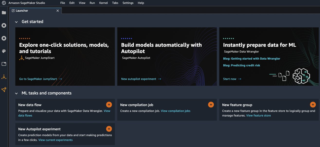
- In the Launcher, choose New data flow. Alternatively, on the File drop-down, choose New, then choose Data Wrangler flow.
- Creating a new flow can take a few minutes. After the flow has been created, you see the Import data page.
Add Amazon EMR as a data source in Data Wrangler
On the Add data source menu, choose Amazon EMR.
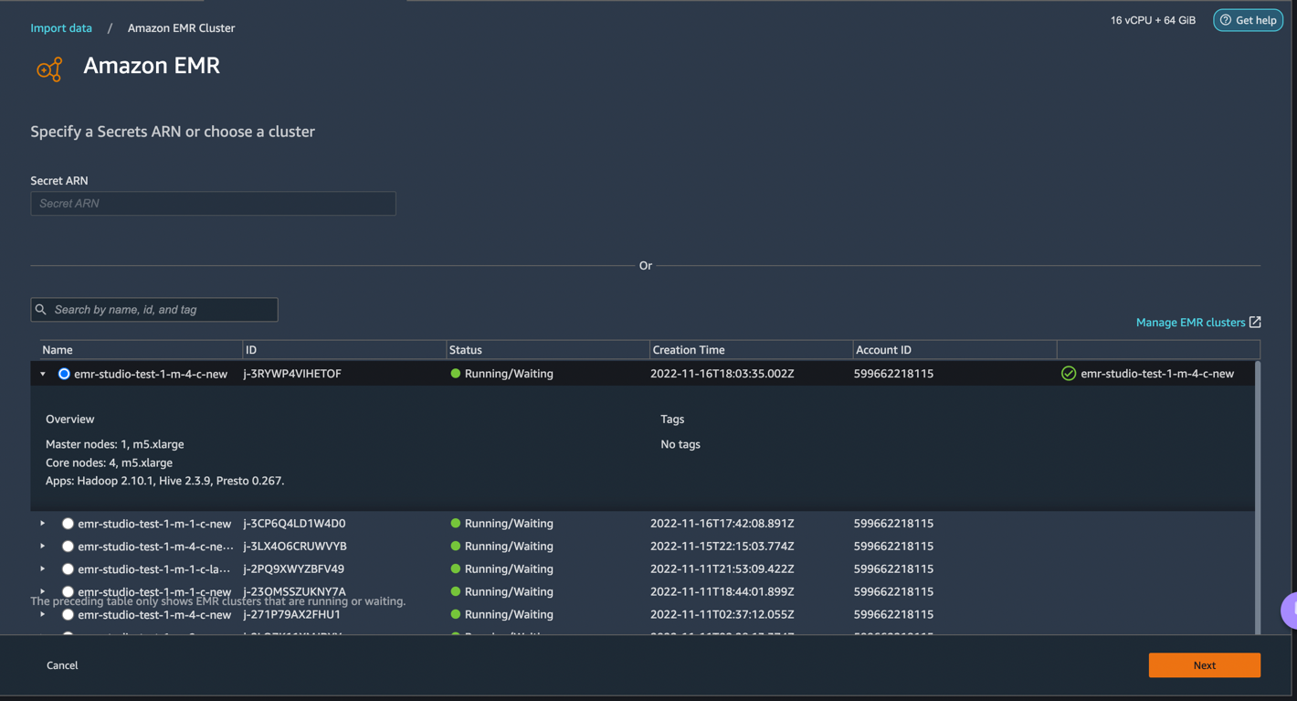
You can browse all the EMR clusters that your Studio execution role has permissions to see. You have two options to connect to a cluster; one is through interactive UI, and the other is to first create a secret using AWS Secrets Manager with JDBC URL, including EMR cluster information, and then provide the stored AWS secret ARN in the UI to connect to Presto. In this blog, we follow the first option. Select one of the following clusters that you want to use. Click on Next, and select endpoints.
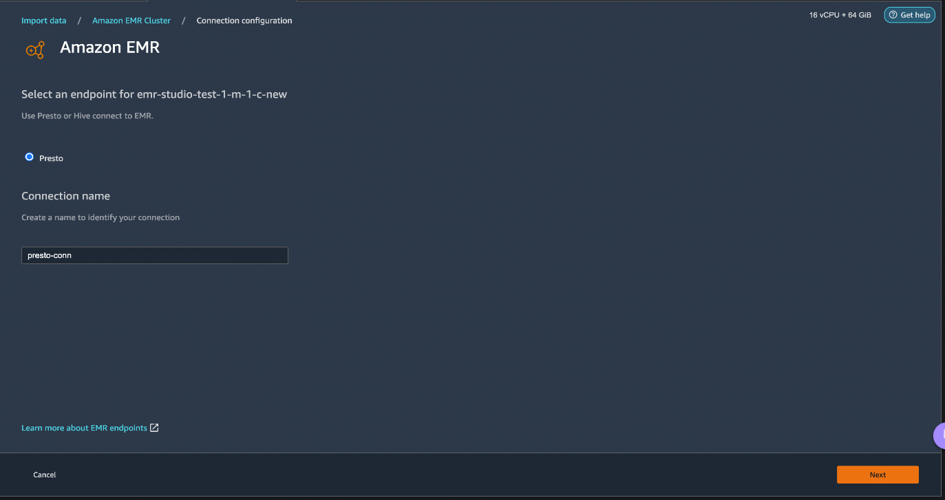
Select Presto, connect to Amazon EMR, create a name to identify your connection, and click Next.
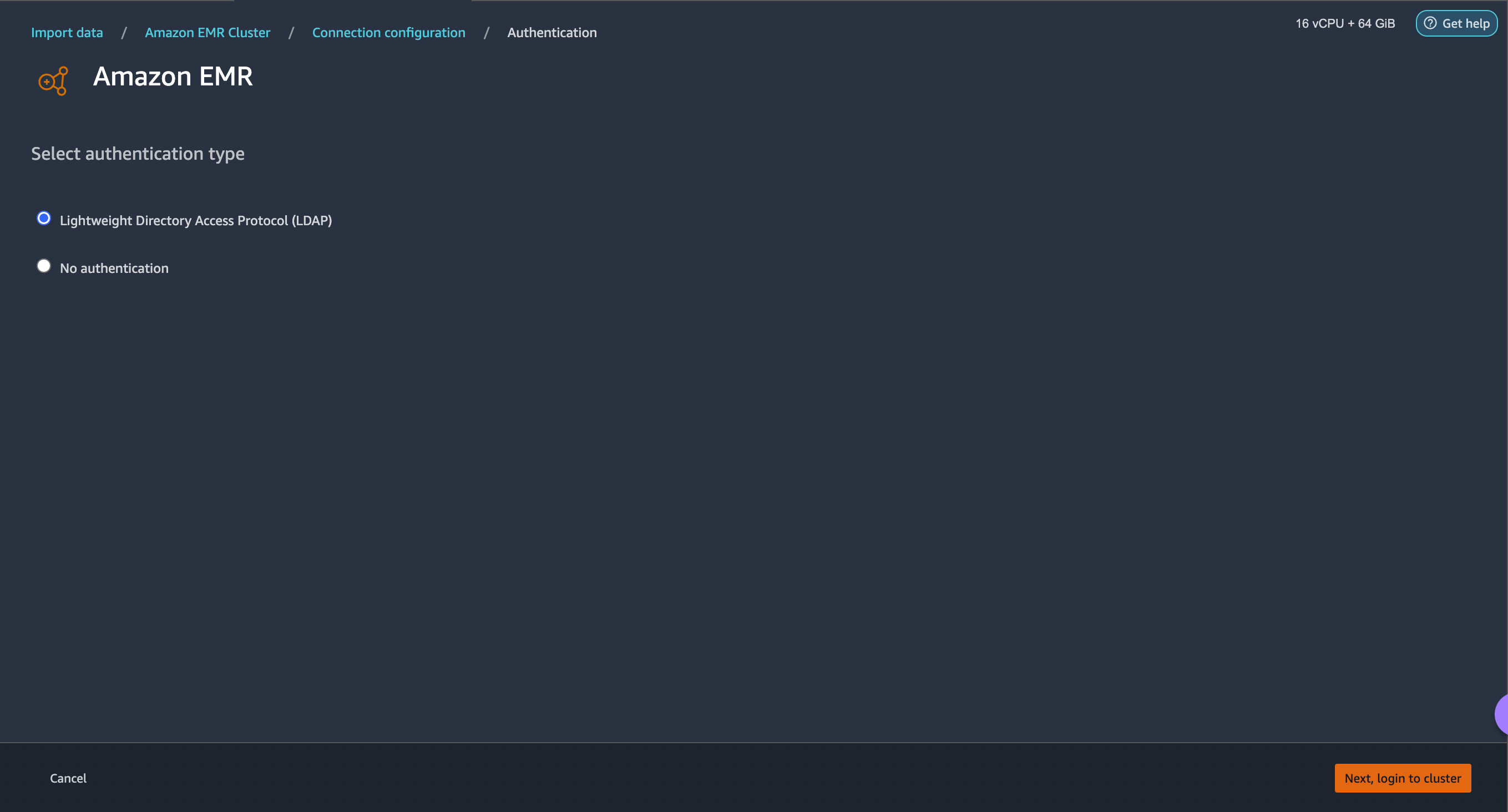
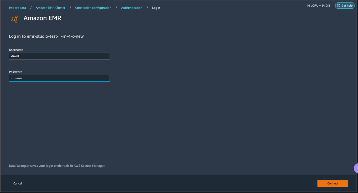
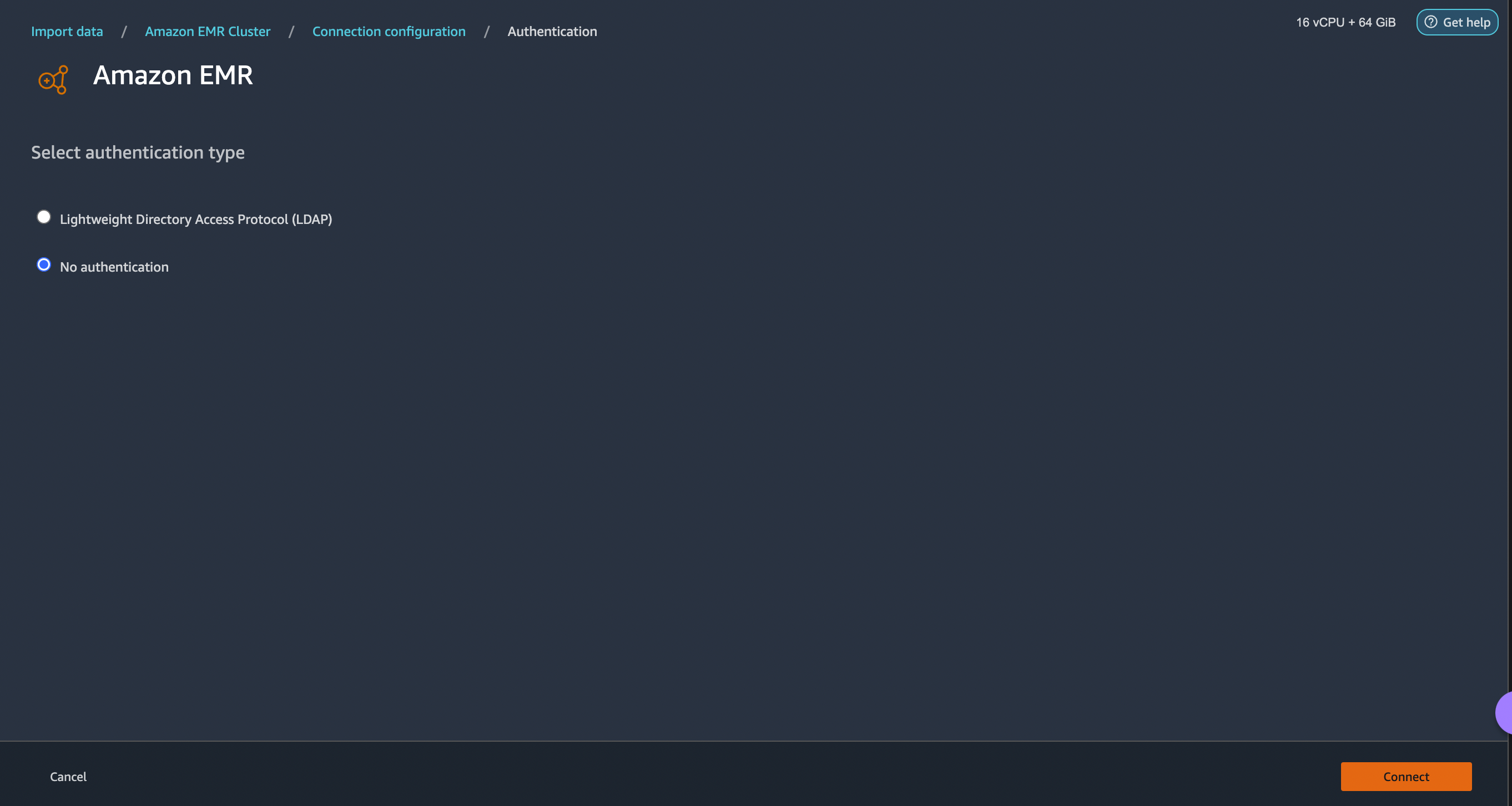
Select Authentication type, either LDAP or No Authentication, and click Connect.
- For Lightweight Directory Access Protocol (LDAP), provide username and password to be authenticated.
- For No Authentication, you will be connected to EMR Presto without providing user credentials within VPC. Enter Data Wrangler’s SQL explorer page for EMR.
Once connected, you can interactively view a database tree and table preview or schema. You can also query, explore, and visualize data from EMR. For preview, you would see a limit of 100 records by default. For customized query, you can provide SQL statements in the query editor box and once you click the Run button, the query will be executed on EMR’s Presto engine.
The Cancel query button allows ongoing queries to be canceled if they are taking an unusually long time.
The last step is to import. Once you are ready with the queried data, you have options to update the sampling settings for the data selection according to the sampling type (FirstK, Random, or Stratified) and sampling size for importing data into Data Wrangler.
Click Import. The prepare page will be loaded, allowing you to add various transformations and essential analysis to the dataset.
Navigate to DataFlow from the top screen and add more steps to the flow as needed for transformations and analysis. You can run a data insight report to identify data quality issues and get recommendations to fix those issues. Let’s look at some example transforms.
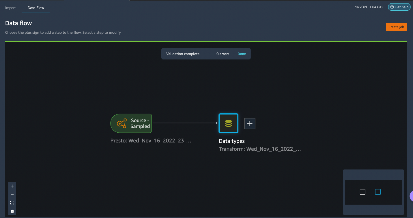
Go to your dataflow, and this is the screen that you should see. It shows us that we are using EMR as a data source using the Presto connector.
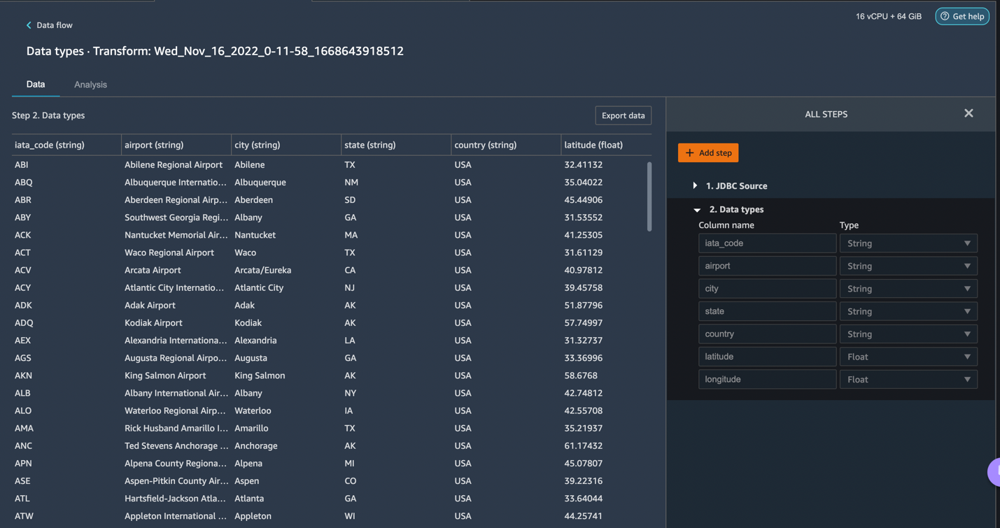
Let’s click on the + button to the right of Data types and select Add transform. When you do that, the following screen should pop up:
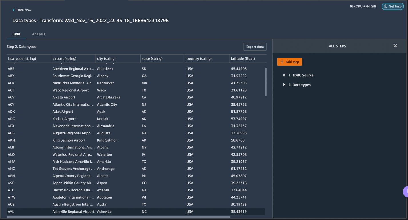
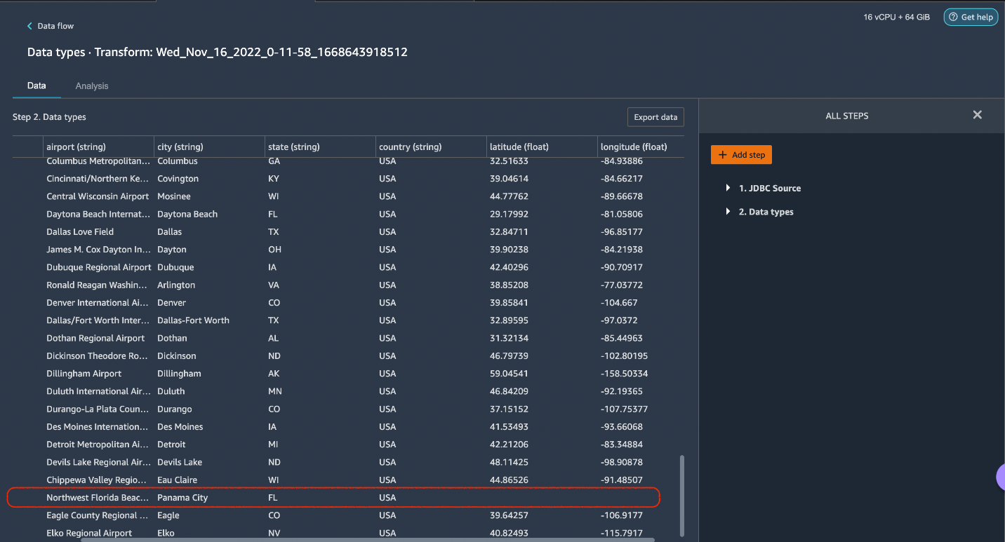
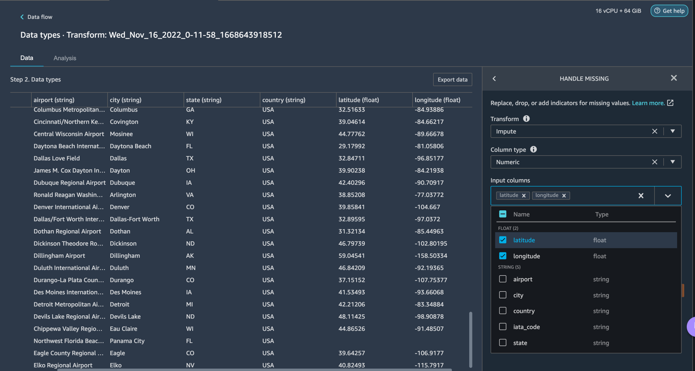
Let’s explore the data. We see that it has multiple features such as iata_code, airport, city, state, country, latitude, and longitude. We can see that the entire dataset is based in one country, which is the US, and there are missing values in Latitude and Longitude. Missing data can cause bias in the estimation of parameters, and it can reduce the representativeness of the samples, so we need to perform some imputation and handle missing values in our dataset.
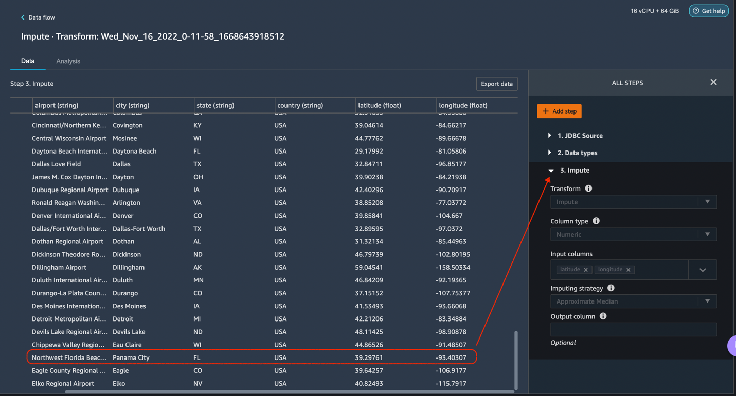
Let’s click on the Add Step button on the navigation bar to the right. Select Handle missing. The configurations can be seen in the following screenshots. Under Transform, select Impute. Select the column type as Numeric and column names Latitude and Longitude. We will be imputing the missing values using an approximate median value. Preview and add the transform.
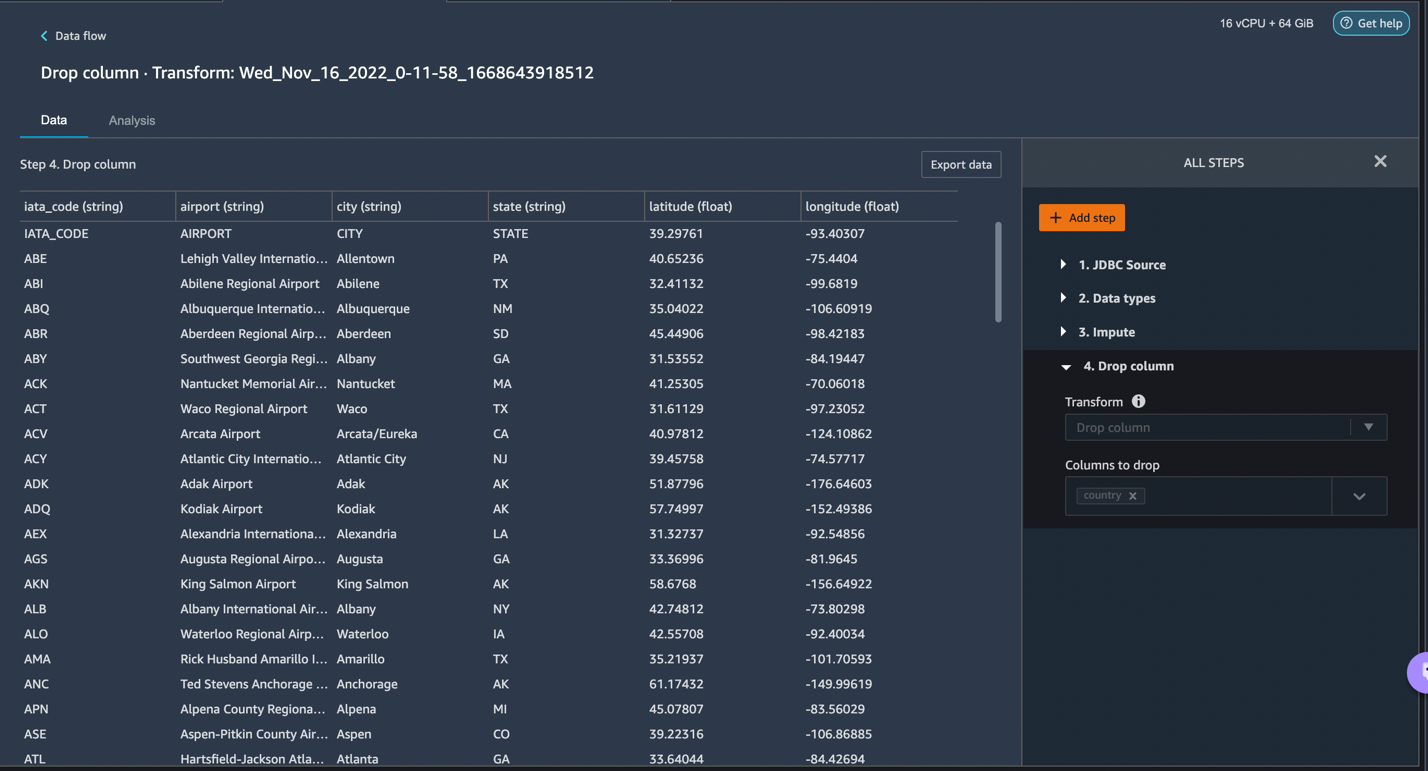
Let us now look at another example transform. When building a machine learning model, columns are removed if they are redundant or don’t help your model. The most common way to remove a column is to drop it. In our dataset, the feature country can be dropped since the dataset is specifically for US airport data. Let’s see how we can manage columns. Let’s click on the Add step button on the navigation bar to the right. Select Manage columns. The configurations can be seen in the following screenshots. Under Transform, select Drop column, and under Columns to drop, select Country.
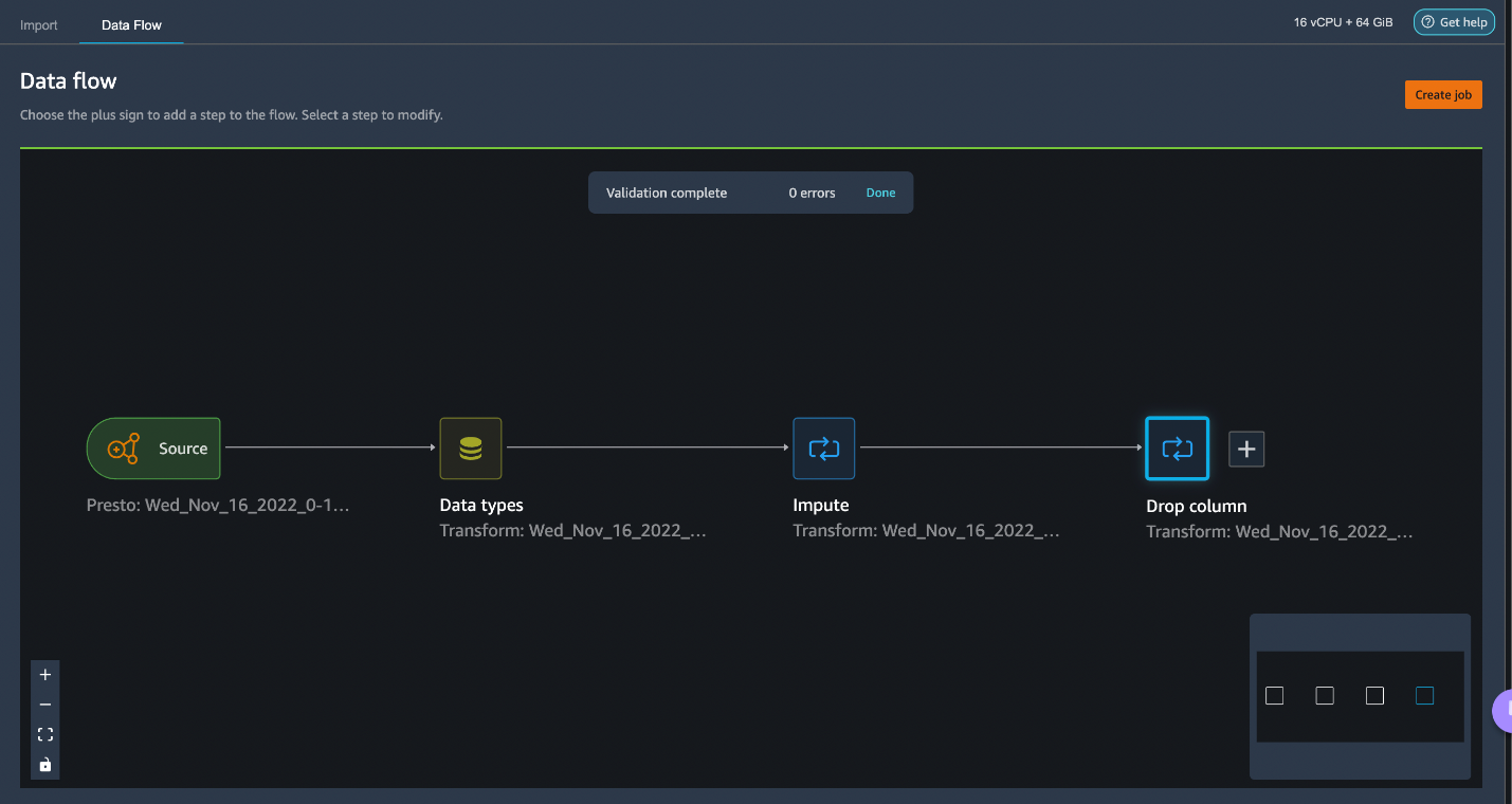
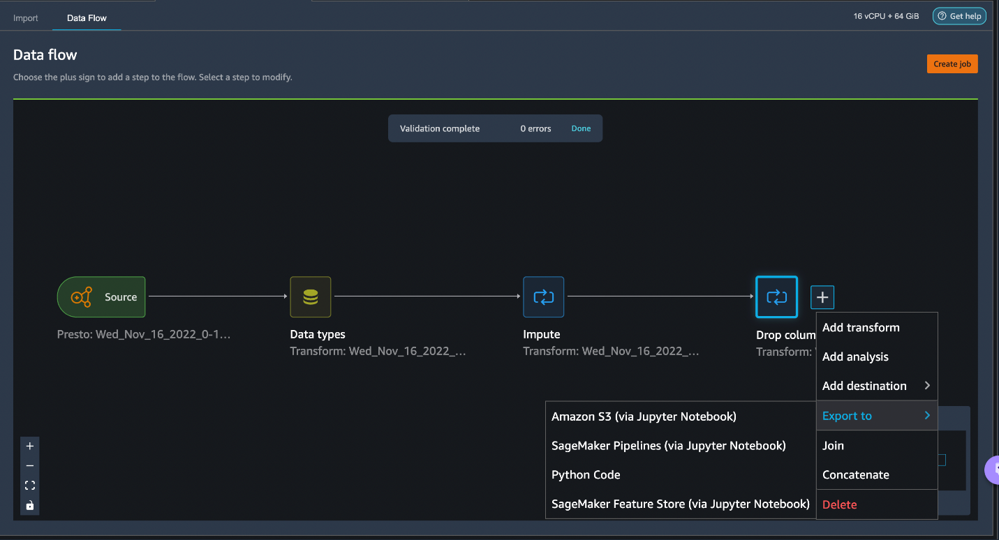
You can continue adding steps based on the different transformations required for your dataset. Let us go back to our data flow. You will now see two more blocks showing the transforms that we performed. In our scenario, you can see Impute and Drop column.
ML practitioners spend a lot of time crafting feature engineering code, applying it to their initial datasets, training models on the engineered datasets, and evaluating model accuracy. Given the experimental nature of this work, even the smallest project will lead to multiple iterations. The same feature engineering code is often run again and again, wasting time and compute resources on repeating the same operations. In large organizations, this can cause an even greater loss of productivity because different teams often run identical jobs or even write duplicate feature engineering code because they have no knowledge of prior work. To avoid the reprocessing of features, we will now export our transformed features to Amazon Feature Store. Let’s click on the + button to the right of Drop column. Select Export to and choose Sagemaker Feature Store (via Jupyter notebook).
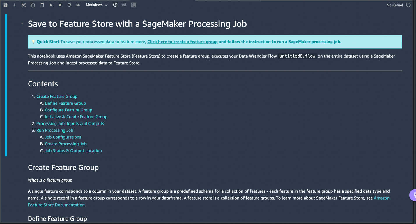
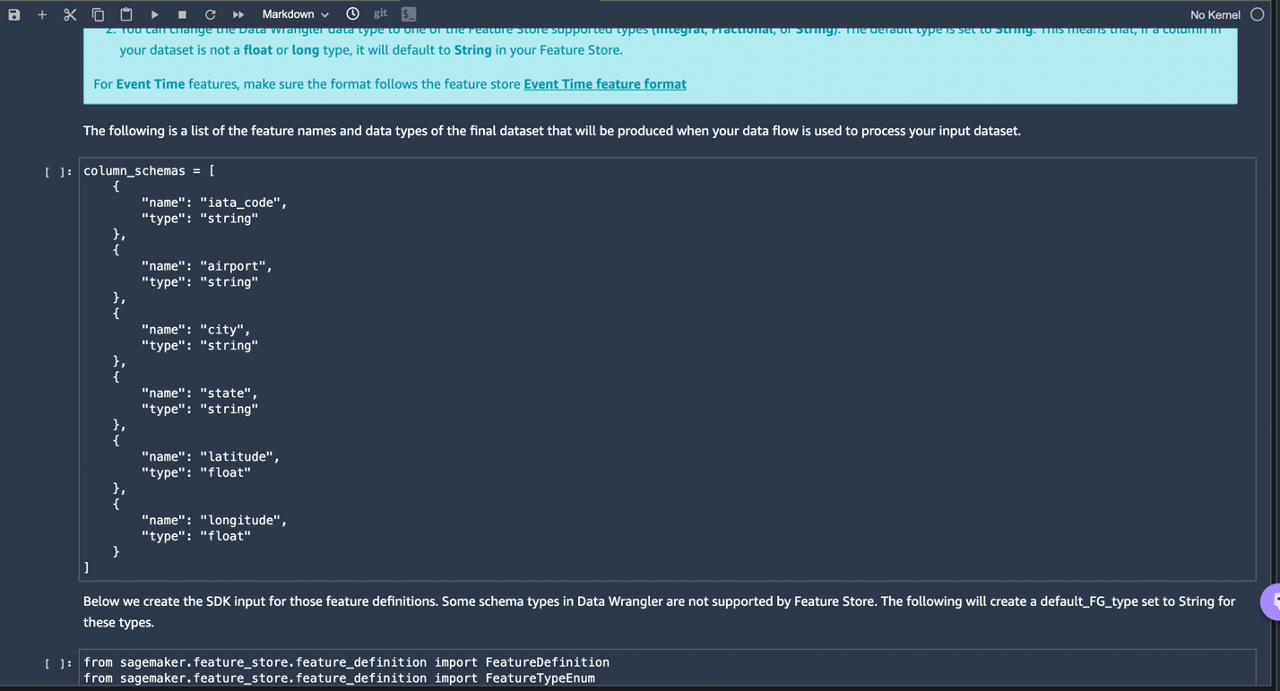
You can easily export your generated features to SageMaker Feature Store by selecting it as the destination. You can save the features into an existing feature group or create a new one.
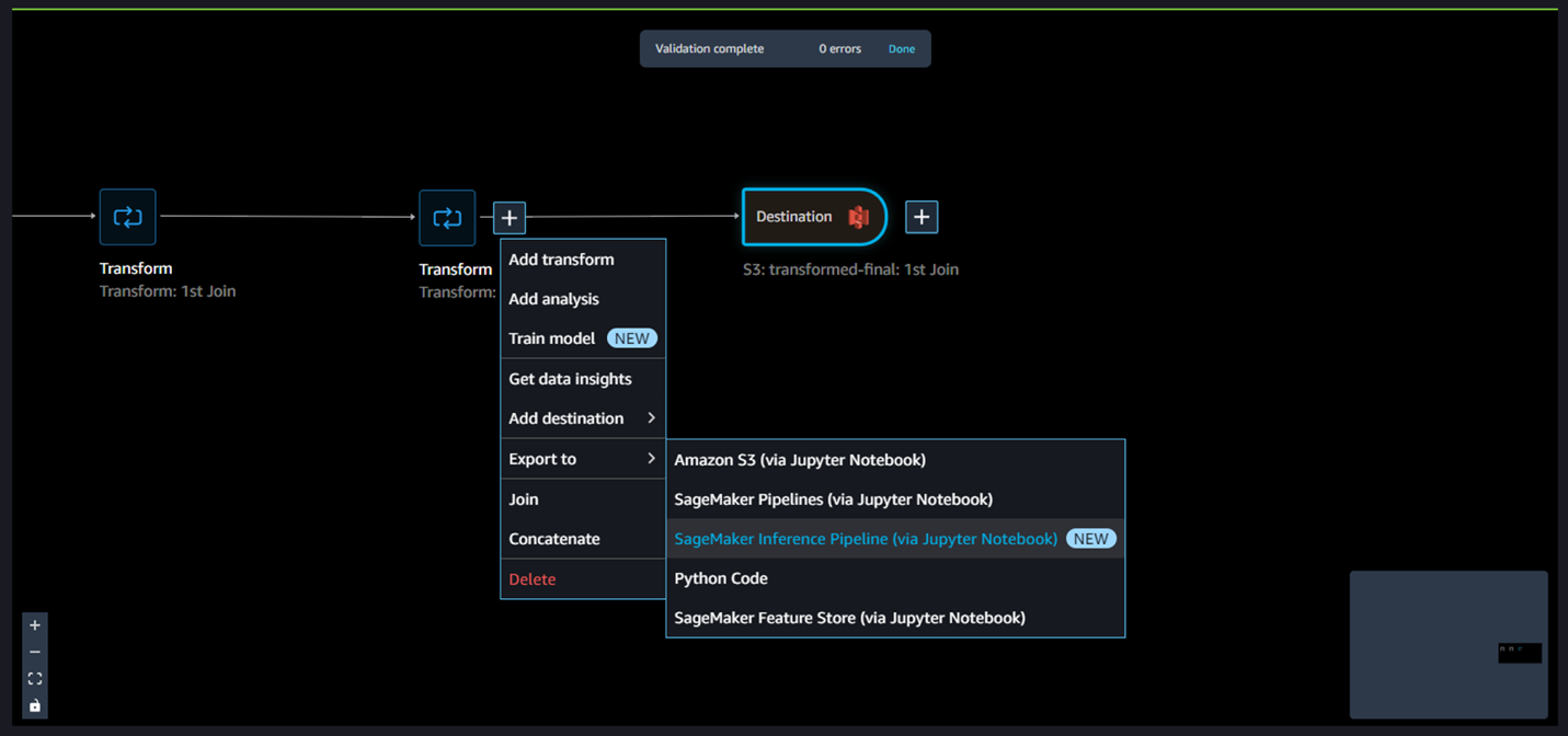
We have now created features with Data Wrangler and easily stored those features in Feature Store. We showed an example workflow for feature engineering in the Data Wrangler UI. Then we saved those features into Feature Store directly from Data Wrangler by creating a new feature group. Finally, we ran a processing job to ingest those features into Feature Store. Data Wrangler and Feature Store together helped us build automatic and repeatable processes to streamline our data preparation tasks with minimum coding required. Data Wrangler also provides us flexibility to automate the same data preparation flow using scheduled jobs. We can also automate training or feature engineering with SageMaker Pipelines (via Jupyter Notebook) and deploy to the Inference endpoint with SageMaker inference pipeline (via Jupyter Notebook).
Clean up
If your work with Data Wrangler is complete, select the stack created from the CloudFormation page and delete it to avoid incurring additional fees.
Conclusion
In this post, we went over how to set up Amazon EMR as a data source in Data Wrangler, how to transform and analyze a dataset, and how to export the results to a data flow for use in a Jupyter notebook. After visualizing our dataset using Data Wrangler’s built-in analytical features, we further enhanced our data flow. The fact that we created a data preparation pipeline without writing a single line of code is significant.
To get started with Data Wrangler, see Prepare ML Data with Amazon SageMaker Data Wrangler, and see the latest information on the Data Wrangler product page.
About the authors
 Ajjay Govindaram is a Senior Solutions Architect at AWS. He works with strategic customers who are using AI/ML to solve complex business problems. His experience lies in providing technical direction as well as design assistance for modest to large-scale AI/ML application deployments. His knowledge ranges from application architecture to big data, analytics, and machine learning. He enjoys listening to music while resting, experiencing the outdoors, and spending time with his loved ones.
 Isha Dua is a Senior Solutions Architect based in the San Francisco Bay Area. She helps AWS enterprise customers grow by understanding their goals and challenges, and guides them on how they can architect their applications in a cloud-native manner while making sure they are resilient and scalable. She’s passionate about machine learning technologies and environmental sustainability.
 Rui Jiang is a Software Development Engineer at AWS based in the New York City area. She is a member of the SageMaker Data Wrangler team helping develop engineering solutions for AWS enterprise customers to achieve their business needs. Outside of work, she enjoys exploring new foods, life fitness, outdoor activities, and traveling.
Exafunction supports AWS Inferentia to unlock best price performance for machine learning inference
Across all industries, machine learning (ML) models are getting deeper, workflows are getting more complex, and workloads are operating at larger scales. Significant effort and resources are put into making these models more accurate since this investment directly results in better products and experiences. On the other hand, making these models run efficiently in production is a non-trivial undertaking that’s often overlooked, despite being key to achieving performance and budget goals. In this post we cover how Exafunction and AWS Inferentia work together to unlock easy and cost-efficient deployment for ML models in production.
Exafunction is a start-up focused on enabling companies to perform ML at scale as efficiently as possible. One of their products is ExaDeploy, an easy-to-use SaaS solution to serve ML workloads at scale. ExaDeploy efficiently orchestrates your ML workloads across mixed resources (CPU and hardware accelerators) to maximize resource utilization. It also takes care of auto scaling, compute colocation, network issues, fault tolerance, and more, to ensure efficient and reliable deployment. AWS Inferentia-based Amazon EC2 Inf1 instances are purpose built to deliver the lowest cost-per-inference in the cloud. ExaDeploy now supports Inf1 instances, which allows users to get both the hardware-based savings of accelerators and the software-based savings of optimized resource virtualization and orchestration at scale.
Solution overview
How ExaDeploy solves for deployment efficiency
To ensure efficient utilization of compute resources, you need to consider proper resource allocation, auto scaling, compute co-location, network cost and latency management, fault tolerance, versioning and reproducibility, and more. At scale, any inefficiencies materially affect costs and latency, and many large companies have addressed these inefficiencies by building internal teams and expertise. However, it’s not practical for most companies to assume this financial and organizational overhead of building generalizable software that isn’t the company’s desired core competency.
ExaDeploy is designed to solve these deployment efficiency pain points, including those seen in some of the most complex workloads such as those in Autonomous Vehicle and natural language processing (NLP) applications. On some large batch ML workloads, ExaDeploy has reduced costs by over 85% without sacrificing on latency or accuracy, with integration time as low as one engineer-day. ExaDeploy has been proven to auto scale and manage thousands of simultaneous hardware accelerator resource instances without any system degradation.
Key features of ExaDeploy include:
- Runs in your cloud: None of your models, inputs, or outputs ever leave your private network. Continue to use your cloud provider discounts.
- Shared accelerator resources: ExaDeploy optimizes the accelerators used by enabling multiple models or workloads to share accelerator resources. It can also identify if multiple workloads are deploying the same model, and then share the model across those workloads, thereby optimizing the accelerator used. Its automatic rebalancing and node draining capabilities maximize utilization and minimize costs.
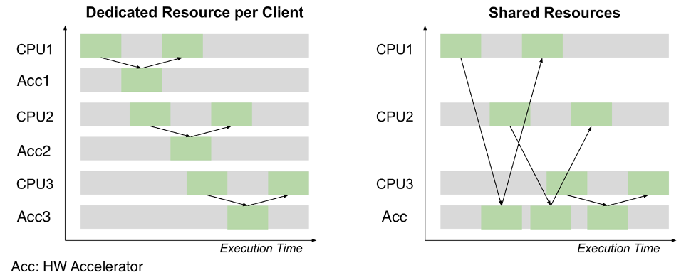
- Scalable serverless deployment model: ExaDeploy auto scales based on accelerator resource saturation. Dynamically scale down to 0 or up to thousands of resources.
- Support for a variety of computation types: You can offload deep learning models from all major ML frameworks as well as arbitrary C++ code, CUDA kernels, custom ops, and Python functions.
- Dynamic model registration and versioning: New models or model versions can be registered and run without having to rebuild or redeploy the system.
- Point-to-point execution: Clients connect directly to remote accelerator resources, which enables low latency and high throughput. They can even store the state remotely.
- Asynchronous execution: ExaDeploy supports asynchronous execution of models, which allows clients to parallelize local computation with remote accelerator resource work.
- Fault-tolerant remote pipelines: ExaDeploy allows clients to dynamically compose remote computations (models, preprocessing, etc.) into pipelines with fault tolerance guarantee. The ExaDeploy system handles pod or node failures with automatic recovery and replay, so that the developers never have to think about ensuring fault tolerance.
- Out-of-the-box monitoring: ExaDeploy provides Prometheus metrics and Grafana dashboards to visualize accelerator resource usage and other system metrics.
ExaDeploy supports AWS Inferentia
AWS Inferentia-based Amazon EC2 Inf1 instances are designed for deep learning specific inference workloads. These instances provide up to 2.3x throughput and up to 70% cost saving compared to the current generation of GPU inference instances.
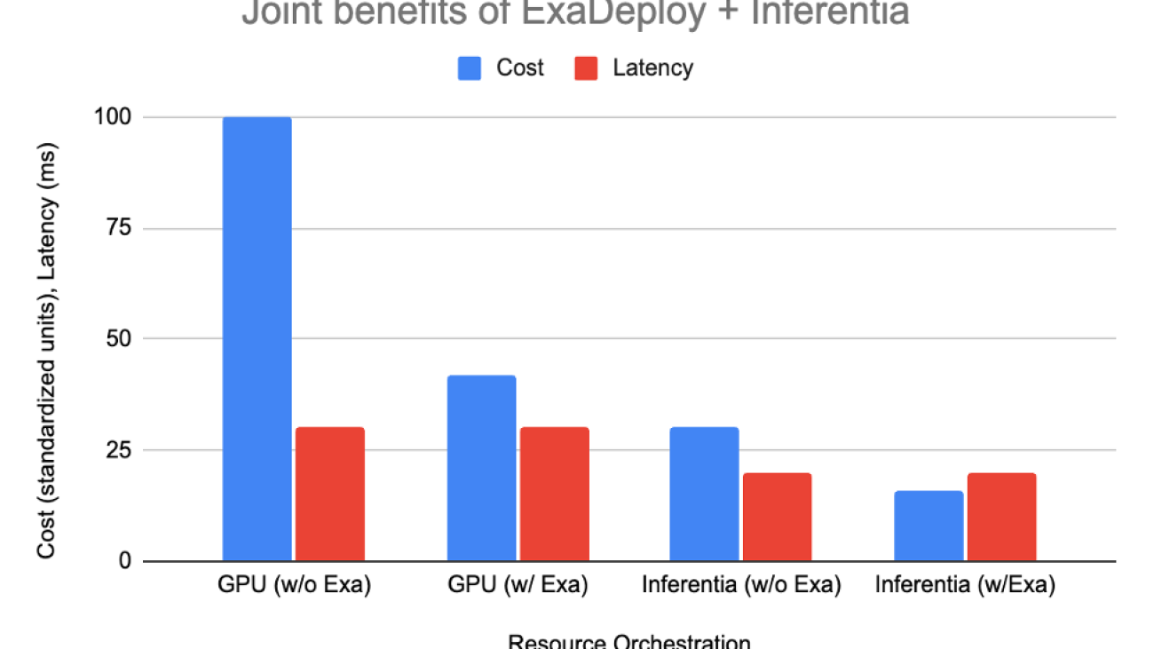
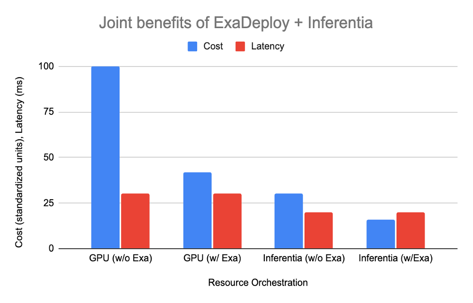
ExaDeploy now supports AWS Inferentia, and together they unlock the increased performance and cost-savings achieved through purpose-built hardware-acceleration and optimized resource orchestration at scale. Let’s look at the combined benefits of ExaDeploy and AWS Inferentia by considering a very common modern ML workload: batched, mixed-compute workloads.
Hypothetical workload characteristics:
- 15 ms of CPU-only pre-process/post-process
- Model inference (15 ms on GPU, 5 ms on AWS Inferentia)
- 10 clients, each make request every 20 ms
- Approximate relative cost of CPU:Inferentia:GPU is 1:2:4 (Based on Amazon EC2 On-Demand pricing for c5.xlarge, inf1.xlarge, and g4dn.xlarge)
The table below shows how each of the options shape up:
| Setup | Resources needed | Cost | Latency |
| GPU without ExaDeploy | 2 CPU, 2 GPU per client (total 20 CPU, 20 GPU) | 100 | 30 ms |
| GPU with ExaDeploy | 8 GPUs shared across 10 clients, 1 CPU per client | 42 | 30 ms |
| AWS Inferentia without ExaDeploy | 1 CPU, 1 AWS Inferentia per client (total 10 CPU, 10 Inferentia) | 30 | 20 ms |
| AWS Inferentia with ExaDeploy | 3 AWS Inferentia shared across 10 clients, 1 CPU per client | 16 | 20 ms |
ExaDeploy on AWS Inferentia example
In this section, we go over the steps to configure ExaDeploy through an example with inf1 nodes on a BERT PyTorch model. We saw an average throughput of 1140 samples/sec for the bert-base model, which demonstrates that little to no overhead was introduced by ExaDeploy for this single model, single workload scenario.
Step 1: Set up an Amazon Elastic Kubernetes Service (Amazon EKS) cluster
An Amazon EKS cluster can be brought up with our Terraform AWS module. For our example, we used an inf1.xlarge for AWS Inferentia.
Step 2: Set up ExaDepoy
The second step is to set up ExaDeploy. In general, the deployment of ExaDeploy on inf1 instances is straightforward. Setup mostly follows the same procedure as it does on graphics processing unit (GPU) instances. The primary difference is to change the model tag from GPU to AWS Inferentia and recompile the model. For example, moving from g4dn to inf1 instances using ExaDeploy’s application programming interfaces (APIs) required only approximately 10 lines of code to be changed.
- One simple method is to use Exafunction’s Terraform AWS Kubernetes module or Helm chart. These deploy the core ExaDeploy components to run in the Amazon EKS cluster.
- Compile model into a serialized format (e.g., TorchScript, TF saved models, ONNX, etc).. For AWS Inferentia, we followed this tutorial.
- Register the compiled model in ExaDeploy’s module repository.
- Prepare the data for the model (i.e., not
ExaDeploy-specific).
- Run the model remotely from the client.
ExaDeploy and AWS Inferentia: Better together
AWS Inferentia is pushing the boundaries of throughput for model inference and delivering lowest cost-per-inference in the cloud. That being said, companies need the proper orchestration to enjoy the price-performance benefits of Inf1 at scale. ML serving is a complex problem that, if addressed in-house, requires expertise that’s removed from company goals and often delays product timelines. ExaDeploy, which is Exafunction’s ML deployment software solution, has emerged as the industry leader. It serves even the most complex ML workloads, while providing smooth integration experiences and support from a world-class team. Together, ExaDeploy and AWS Inferentia unlock increased performance and cost-savings for inference workloads at scale.
Conclusion
In this post, we showed you how Exafunction supports AWS Inferentia for performance ML. For more information on building applications with Exafunction, visit Exafunction. For best practices on building deep learning workloads on Inf1, visit Amazon EC2 Inf1 instances.
About the Authors
Nicholas Jiang, Software Engineer, Exafunction
Jonathan Ma, Software Engineer, Exafunction
Prem Nair, Software Engineer, Exafunction
Anshul Ramachandran, Software Engineer, Exafunction
Shruti Koparkar, Sr. Product Marketing Manager, AWS
Formation of Robust Bound States of Interacting Photons
When quantum computers were first proposed, they were hoped to be a way to better understand the quantum world. With a so-called “quantum simulator,” one could engineer a quantum computer to investigate how various quantum phenomena arise, including those that are intractable to simulate with a classical computer.
But making a useful quantum simulator has been a challenge. Until now, quantum simulations with superconducting qubits have predominantly been used to verify pre-existing theoretical predictions and have rarely explored or discovered new phenomena. Only a few experiments with trapped ions or cold atoms have revealed new insights. Superconducting qubits, even though they are one of the main candidates for universal quantum computing and have demonstrated computational capabilities beyond classical reach, have so far not delivered on their potential for discovery.
In “Formation of Robust Bound States of Interacting Photons”, published in Nature, we describe a previously unpredicted phenomenon first discovered through experimental investigation. First, we present the experimental confirmation of the theoretical prediction of the existence of a composite particle of interacting photons, or a bound state, using the Google Sycamore quantum processor. Second, while studying this system, we discovered that even though one might guess the bound states to be fragile, they remain robust to perturbations that we expected to have otherwise destroyed them. Not only does this open the possibility of designing systems that leverage interactions between photons, it also marks a step forward in the use of superconducting quantum processors to make new scientific discoveries by simulating non-equilibrium quantum dynamics.
Overview
Photons, or quanta of electromagnetic radiation like light and microwaves, typically don’t interact. For example, two intersecting flashlight beams will pass through one another undisturbed. In many applications, like telecommunications, the weak interactions of photons is a valuable feature. For other applications, such as computers based on light, the lack of interactions between photons is a shortcoming.
In a quantum processor, the qubits host microwave photons, which can be made to interact through two-qubit operations. This allows us to simulate the XXZ model, which describes the behavior of interacting photons. Importantly, this is one of the few examples of integrable models, i.e., one with a high degree of symmetry, which greatly reduces its complexity. When we implement the XXZ model on the Sycamore processor, we observe something striking: the interactions force the photons into bundles known as bound states.
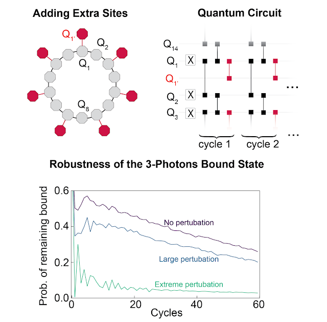
Using this well-understood model as a starting point, we then push the study into a less-understood regime. We break the high level of symmetries displayed in the XXZ model by adding extra sites that can be occupied by the photons, making the system no longer integrable. While this nonintegrable regime is expected to exhibit chaotic behavior where bound states dissolve into their usual, solitary selves, we instead find that they survive!
Bound Photons
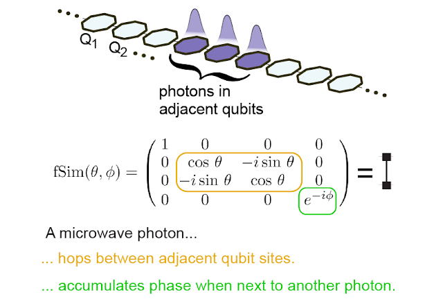
To engineer a system that can support the formation of bound states, we study a ring of superconducting qubits that host microwave photons. If a photon is present, the value of the qubit is “1”, and if not, the value is “0”. Through the so-called “fSim” quantum gate, we connect neighboring sites, allowing the photons to hop around and interact with other photons on the nearest-neighboring sites.
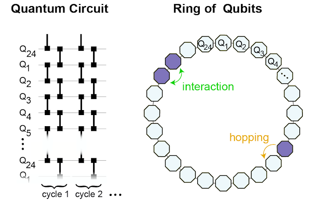 |
| We implement the fSim gate between neighboring qubits (left) to effectively form a ring of 24 interconnected qubits on which we simulate the behavior of the interacting photons (right). |
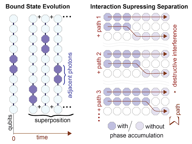
The interactions between the photons affect their so-called “phase.” This phase keeps track of the oscillation of the photon’s wavefunction. When the photons are non-interacting, their phase accumulation is rather uninteresting. Like a well-rehearsed choir, they’re all in sync with one another. In this case, a photon that was initially next to another photon can hop away from its neighbor without getting out of sync. Just as every person in the choir contributes to the song, every possible path the photon can take contributes to the photon’s overall wavefunction. A group of photons initially clustered on neighboring sites will evolve into a superposition of all possible paths each photon might have taken.
When photons interact with their neighbors, this is no longer the case. If one photon hops away from its neighbor, its rate of phase accumulation changes, becoming out of sync with its neighbors. All paths in which the photons split apart overlap, leading to destructive interference. It would be like each choir member singing at their own pace — the song itself gets washed out, becoming impossible to discern through the din of the individual singers. Among all the possible configuration paths, the only possible scenario that survives is the configuration in which all photons remain clustered together in a bound state. This is why interaction can enhance and lead to the formation of a bound state: by suppressing all other possibilities in which photons are not bound together.
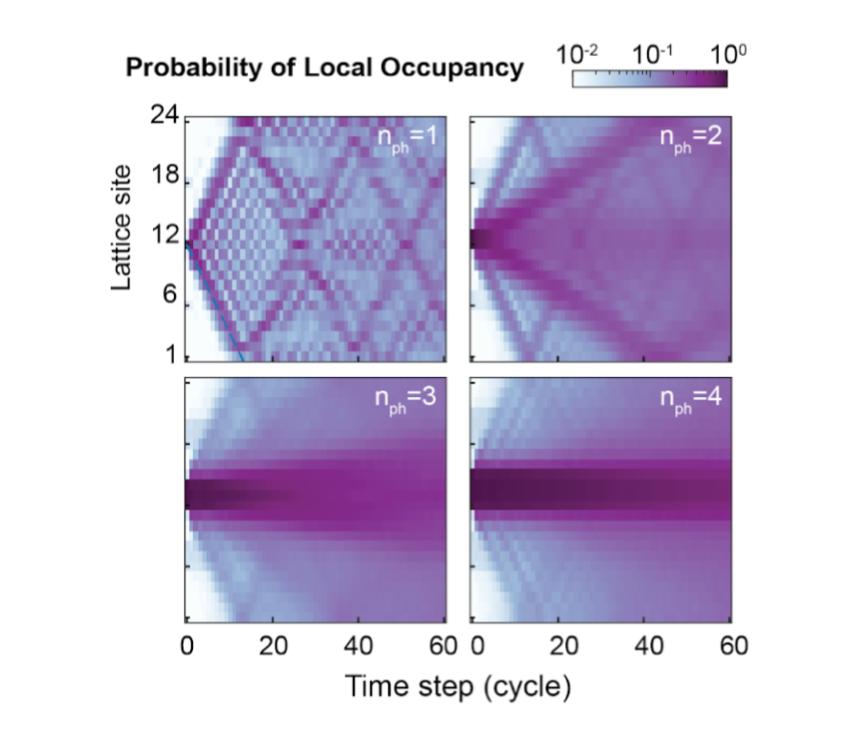
In our processor, we start by putting two to five photons on adjacent sites (i.e., initializing two to five adjacent qubits in “1”, and the remaining qubits in “0”), and then study how they propagate. First, we notice that in the theoretically predicted parameter regime, they remain stuck together. Next, we find that the larger bound states move more slowly around the ring, consistent with the fact that they are “heavier”. This can be seen in the plot above where the lattice sites closest to Site 12, the initial position of the photons, remain darker than the others with increasing number of photons (nph) in the bound state, indicating that with more photons bound together there is less propagation around the ring.
Bound States Behave Like Single Composite Particles
To more rigorously show that the bound states indeed behave as single particles with well-defined physical properties, we devise a method to measure how the energy of the particles changes with momentum, i.e., the energy-momentum dispersion relation.
To measure the energy of the bound state, we use the fact that the energy difference between two states determines how fast their relative phase grows with time. Hence, we prepare the bound state in a superposition with the state that has no photons, and measure their phase difference as a function of time and space. Then, to convert the result of this measurement to a dispersion relation, we utilize a Fourier transform, which translates position and time into momentum and energy, respectively. We’re left with the familiar energy-momentum relationship of excitations in a lattice.
 |
| Spectroscopy of bound states. We compare the phase accumulation of an n-photon bound state with that of the vacuum (no photons) as a function of lattice site and time. A 2D Fourier transform yields the dispersion relation of the bound-state quasiparticle. |
Breaking Integrability
The above system is “integrable,” meaning that it has a sufficient number of conserved quantities that its dynamics are constrained to a small part of the available computational space. In such integrable regimes, the appearance of bound states is not that surprising. In fact, bound states in similar systems were predicted in 2012, then observed in 2013. However, these bound states are fragile and their existence is usually thought to derive from integrability. For more complex systems, there is less symmetry and integrability is quickly lost. Our initial idea was to probe how these bound states disappear as we break integrability to better understand their rigidity.
To break integrability, we modify which qubits are connected with fSim gates. We add qubits so that at alternating sites, in addition to hopping to each of its two nearest-neighboring sites, a photon can also hop to a third site oriented radially outward from the ring.
While a bound state is constrained to a very small part of phase space, we expected that the chaotic behavior associated with integrability breaking would allow the system to explore the phase space more freely. This would cause the bound states to break apart. We find that this is not the case. Even when the integrability breaking is so strong that the photons are equally likely to hop to the third site as they are to hop to either of the two adjacent ring sites, the bound state remains intact, up to the decoherence effect that makes them slowly decay (see paper for details).
Conclusion
We don’t yet have a satisfying explanation for this unexpected resilience. We speculate that it may be related to a phenomenon called prethermalization, where incommensurate energy scales in the system can prevent a system from reaching thermal equilibrium as quickly as it otherwise would. We believe further investigations will hopefully lead to new insights into many-body quantum physics, including the interplay of prethermalization and integrability.
Acknowledgements
We would like to thank our Quantum Science Communicator Katherine McCormick for her help writing this blog post.
Damage assessment using Amazon SageMaker geospatial capabilities and custom SageMaker models
In this post, we show how to train, deploy, and predict natural disaster damage with Amazon SageMaker with geospatial capabilities. We use the new SageMaker geospatial capabilities to generate new inference data to test the model. Many government and humanitarian organizations need quick and accurate situational awareness when a disaster strikes. Knowing the severity, cause, and location of damage can assist in the first responder’s response strategy and decision-making. The lack of accurate and timely information can contribute to an incomplete or misdirected relief effort.
As the frequency and severity of natural disasters increases, it’s important that we equip decision-makers and first responders with fast and accurate damage assessment. In this example, we use geospatial imagery to predict natural disaster damage. Geospatial data can be used in the immediate aftermath of a natural disaster for rapidly identifying damage to buildings, roads, or other critical infrastructure. In this post, we show you how to train and deploy a geospatial segmentation model to be used for disaster damage classification. We break down the application into three topics: model training, model deployment, and inference.
Model training
In this use case, we built a custom PyTorch model using Amazon SageMaker for image segmentation of building damage. The geospatial capabilities in SageMaker include trained models for you to utilize. These built-in models include cloud segmentation and removal, and land cover segmentation. For this post, we train a custom model for damage segmentation. We first trained the SegFormer model on data from the xView2 competition. The SegFormer is a transformer-based architecture that was introduced in the 2021 paper SegFormer: Simple and Efficient Design for Semantic Segmentation with Transformers. It’s based on the transformer architectures that are quite popular with natural language processing workloads; however, the SegFormer architecture is built for semantic segmentation. It combines both the transformer-based encoder and a lightweight decoder. This allows for better performance than previous methods, while providing significantly smaller model sizes than previous methods. Both pre-trained and untrained SegFormer models are available from the popular Hugging Face transformer library. For this use case, we download a pre-trained SegFormer architecture and train it on a new dataset.
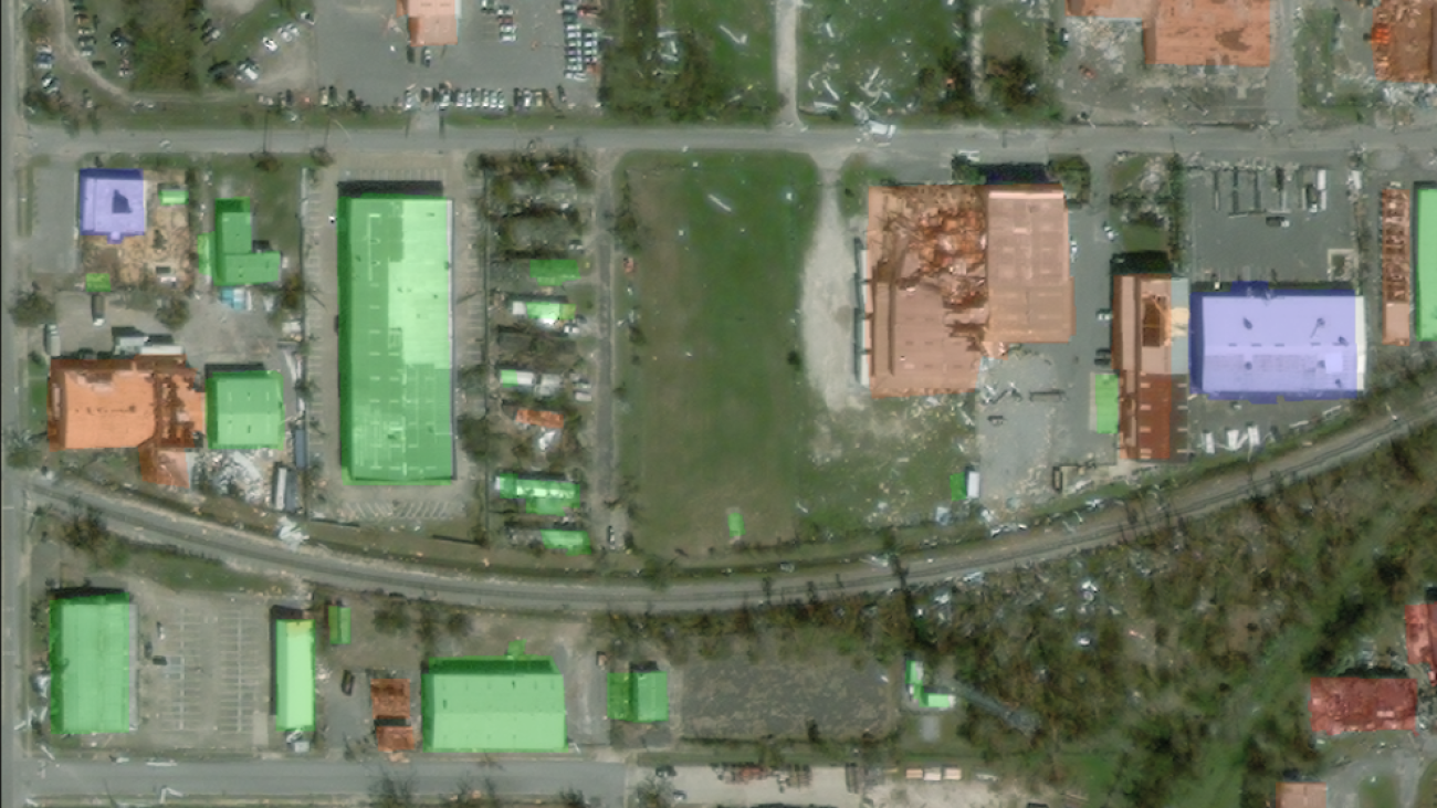
The dataset used in this example comes from the xView2 data science competition. This competition released the xBD dataset, one of the largest and highest-quality publicly available datasets of high-resolution satellite imagery annotated with building location and damage scores (classes) before and after natural disasters. The dataset contains data from 15 countries including 6 types of disasters (earthquake/tsunami, flood, volcanic eruption, wildfire, wind) with geospatial data containing 850,736 building annotations across 45,362 km^2 of imagery. The following image shows an example of the dataset. This image shows the post-disaster image with the building damage segmentation mask overlayed. Each image includes the following: pre-disaster satellite image, pre-disaster building segmentation mask, post-disaster satellite image, and post-disaster building segmentation mask with damage classes.
In this example, we only use the pre- and post-disaster imagery to predict the post-disaster damage classification (segmentation mask). We don’t use the pre-disaster building segmentation masks. This approach was selected for simplicity. There are other options for approaching this dataset. A number of the winning approaches for the xView2 competition used a two-step solution: first, predict the pre-disaster building outline segmentation mask. The building outlines and the post-damage images are then used as input for predicting the damage classification. We leave this to the reader to explore other modeling approaches to improve classification and detection performance.
The pre-trained SegFormer architecture is built to accept a single three-color channel image as input and outputs a segmentation mask. There are a number of ways we could have modified the model to accept both the pre- and post-satellite images as input, however, we used a simple stacking technique to stack both images together into a six-color channel image. We trained the model using standard augmentation techniques on the xView2 training dataset to predict the post-disaster segmentation mask. Note that we did resize all the input images from 1024 to 512 pixels. This was to further reduce spatial resolution of the training data. The model was trained with SageMaker using a single p3.2xlarge GPU based instance. An example of the trained model output is shown in the following figures. The first set of images are the pre- and post-damage images from the validation set.
The following figures show the predicted damage mask and ground truth damage mask.
At first glance, it seems like the model doesn’t perform well as compared to the ground truth data. Many of the buildings are incorrectly classified, confusing minor damage for no damage and showing multiple classifications for a single building outline. However, one interesting finding when reviewing the model performance is that it appears to have learned to localize the building damage classification. Each building can be classified into No Damage, Minor Damage, Major Damage, or Destroyed. The predicted damage mask shows that the model has classified the large building in the middle into mostly No Damage, but the top right corner is classified as Destroyed. This sub-building damage localization can further assist responders by showing the localized damage per building.
Model deployment
The trained model was then deployed to an asynchronous SageMaker inference endpoint. Note that we chose an asynchronous endpoint to allow for longer inference times, larger payload input sizes, and the ability to scale the endpoint down to zero instances (no charges) when not in use. The following figure shows the high-level code for asynchronous endpoint deployment. We first compress the saved PyTorch state dictionary and upload the compressed model artifacts to Amazon Simple Storage Service (Amazon S3). We create a SageMaker PyTorch model pointing to our inference code and model artifacts. The inference code is required to load and serve our model. For more details on the required custom inference code for a SageMaker PyTorch model, refer to Use PyTorch with the SageMaker Python SDK.
The following figure shows the code for the auto scaling policy for the asynchronous inference endpoint.
Note that there are other endpoint options, such as real time, batch, and serverless, that could be used for your application. You’ll want to pick the option that is best suited for the use case and recall that Amazon SageMaker Inference Recommender is available to help recommend machine learning (ML) endpoint configurations.
Model inference
With the trained model deployed, we can now use SageMaker geospatial capabilities to gather data for inference. With SageMaker geospatial capabilities, several built-in models are available out of the box. In this example, we use the band stacking operation for stacking the red, green, and blue color channels for our earth observation job. The job gathers the data from the Sentinel-2 dataset. To configure an earth observation job, we first need the coordinates of the location of interest. Second, we need the time range of the observation. With this we can now submit an earth observation job using the stacking feature. Here we stack the red, green, and blue bands to produce a color image. The following figure shows the job configuration used to generate data from the floods in Rochester, Australia, in mid-October 2022. We utilize images from before and after the disaster as input to our trained ML model.
After the job configuration is defined, we can submit the job. When the job is complete, we export the results to Amazon S3. Note that we can only export the results after the job has completed. The results of the job can be exported to an Amazon S3 location specified by the user in the export job configuration. Now with our new data in Amazon S3, we can get damage predictions using the deployed model. We first read the data into memory and stack the pre- and post-disaster imagery together.
The results of the segmentation mask for the Rochester floods are shown in the following images. Here we can see that the model has identified locations within the flooded region as likely damaged. Note also that the spatial resolution of the inference image is different than the training data. Increasing the spatial resolution could help model performance; however, this is less of an issue for the SegFormer model as it is for other models due to the multiscale model architecture.
Conclusion
In this post, we showed how to train, deploy, and predict natural disaster damage with SageMaker with geospatial capabilities. We used the new SageMaker geospatial capabilities to generate new inference data to test the model. The code for this post is in the process of being released, and this post will be updated with links to the full training, deployment, and inference code. This application allows for first responders, governments, and humanitarian organizations to optimize their response, providing critical situational awareness immediately following a natural disaster. This application is only one example of what is possible with modern ML tools such as SageMaker.
Try SageMaker geospatial capabilities today using your own models; we look forward to seeing what you build next.
About the author
 Aaron Sengstacken is a machine learning specialist solutions architect at Amazon Web Services. Aaron works closely with public sector customers of all sizes to develop and deploy production machine learning applications. He is interested in all things machine learning, technology, and space exploration.


