Learn how Amazon uses machine-learning techniques to modify different aspects of speech — tone, phrasing, intonation, expressiveness, and accent — to create unique Alexa responses.Read More
How VMware built an MLOps pipeline from scratch using GitLab, Amazon MWAA, and Amazon SageMaker
This post is co-written with Mahima Agarwal, Machine Learning Engineer, and Deepak Mettem, Senior Engineering Manager, at VMware Carbon Black
VMware Carbon Black is a renowned security solution offering protection against the full spectrum of modern cyberattacks. With terabytes of data generated by the product, the security analytics team focuses on building machine learning (ML) solutions to surface critical attacks and spotlight emerging threats from noise.
It is critical for the VMware Carbon Black team to design and build a custom end-to-end MLOps pipeline that orchestrates and automates workflows in the ML lifecycle and enables model training, evaluations, and deployments.
There are two main purposes for building this pipeline: support the data scientists for late-stage model development, and surface model predictions in the product by serving models in high volume and in real-time production traffic. Therefore, VMware Carbon Black and AWS chose to build a custom MLOps pipeline using Amazon SageMaker for its ease of use, versatility, and fully managed infrastructure. We orchestrate our ML training and deployment pipelines using Amazon Managed Workflows for Apache Airflow (Amazon MWAA), which enables us to focus more on programmatically authoring workflows and pipelines without having to worry about auto scaling or infrastructure maintenance.
With this pipeline, what once was Jupyter notebook-driven ML research is now an automated process deploying models to production with little manual intervention from data scientists. Earlier, the process of training, evaluating, and deploying a model could take over a day; with this implementation, everything is just a trigger away and has reduced the overall time to few minutes.
In this post, VMware Carbon Black and AWS architects discuss how we built and managed custom ML workflows using Gitlab, Amazon MWAA, and SageMaker. We discuss what we achieved so far, further enhancements to the pipeline, and lessons learned along the way.
Solution overview
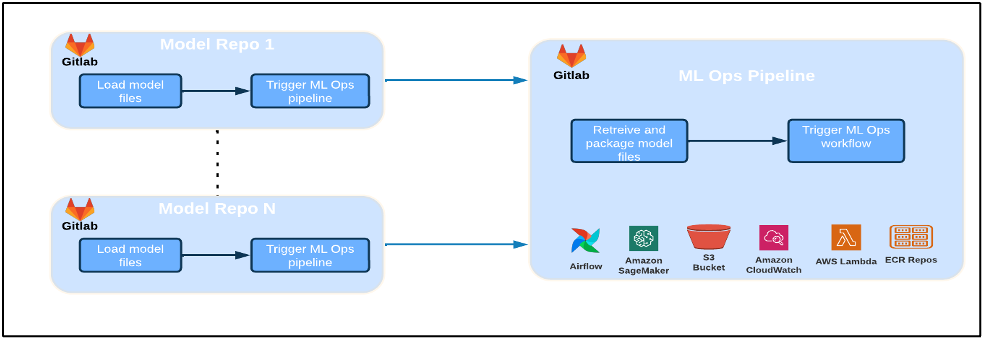
The following diagram illustrates the ML platform architecture.
High level Solution Design
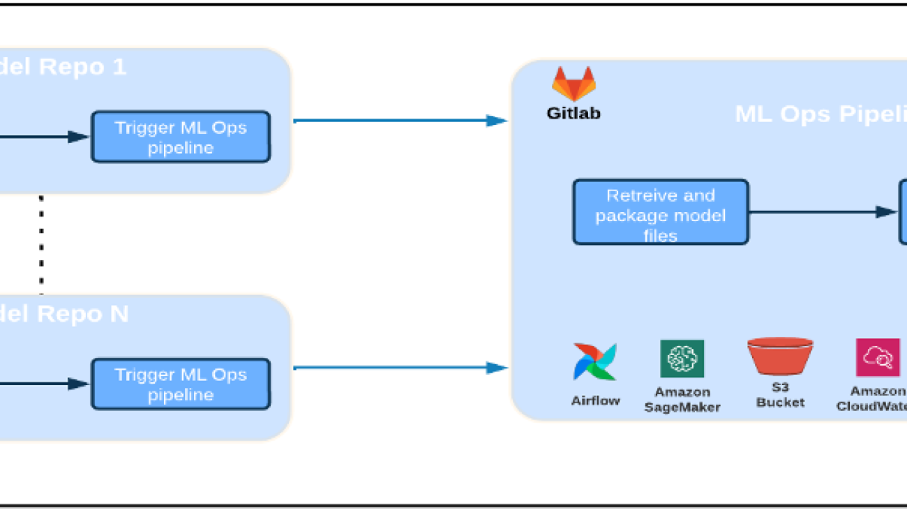
This ML platform was envisioned and designed to be consumed by different models across various code repositories. Our team uses GitLab as a source code management tool to maintain all the code repositories. Any changes in the model repository source code are continuously integrated using the Gitlab CI, which invokes the subsequent workflows in the pipeline (model training, evaluation, and deployment).
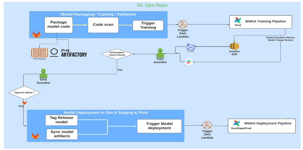
The following architecture diagram illustrates the end-to-end workflow and the components involved in our MLOps pipeline.
End-To-End Workflow
The ML model training, evaluation, and deployment pipelines are orchestrated using Amazon MWAA, referred to as a Directed Acyclic Graph (DAG). A DAG is a collection of tasks together, organized with dependencies and relationships to say how they should run.
At a high level, the solution architecture includes three main components:
- ML pipeline code repository
- ML model training and evaluation pipeline
- ML model deployment pipeline
Let’s discuss how these different components are managed and how they interact with each other.
ML pipeline code repository
After the model repo integrates the MLOps repo as their downstream pipeline, and a data scientist commits code in their model repo, a GitLab runner does standard code validation and testing defined in that repo and triggers the MLOps pipeline based on the code changes. We use Gitlab’s multi-project pipeline to enable this trigger across different repos.
The MLOps GitLab pipeline runs a certain set of stages. It conducts basic code validation using pylint, packages the model’s training and inference code within the Docker image, and publishes the container image to Amazon Elastic Container Registry (Amazon ECR). Amazon ECR is a fully managed container registry offering high-performance hosting, so you can reliably deploy application images and artifacts anywhere.
ML model training and evaluation pipeline
After the image is published, it triggers the training and evaluation Apache Airflow pipeline through the AWS Lambda function. Lambda is a serverless, event-driven compute service that lets you run code for virtually any type of application or backend service without provisioning or managing servers.
After the pipeline is successfully triggered, it runs the Training and Evaluation DAG, which in turn starts the model training in SageMaker. At the end of this training pipeline, the identified user group gets a notification with the training and model evaluation results over email through Amazon Simple Notification Service (Amazon SNS) and Slack. Amazon SNS is fully managed pub/sub service for A2A and A2P messaging.
After meticulous analysis of the evaluation results, the data scientist or ML engineer can deploy the new model if the performance of the newly trained model is better compared to the previous version. The performance of the models is evaluated based on the model-specific metrics (such as F1 score, MSE, or confusion matrix).
ML model deployment pipeline
To start deployment, the user starts the GitLab job that triggers the Deployment DAG through the same Lambda function. After the pipeline runs successfully, it creates or updates the SageMaker endpoint with the new model. This also sends a notification with the endpoint details over email using Amazon SNS and Slack.
In the event of failure in either of the pipelines, users are notified over the same communication channels.
SageMaker offers real-time inference that is ideal for inference workloads with low latency and high throughput requirements. These endpoints are fully managed, load balanced, and auto scaled, and can be deployed across multiple Availability Zones for high availability. Our pipeline creates such an endpoint for a model after it runs successfully.
In the following sections, we expand on the different components and dive into the details.
GitLab: Package models and trigger pipelines
We use GitLab as our code repository and for the pipeline to package the model code and trigger downstream Airflow DAGs.
Multi-project pipeline
The multi-project GitLab pipeline feature is used where the parent pipeline (upstream) is a model repo and the child pipeline (downstream) is the MLOps repo. Each repo maintains a .gitlab-ci.yml, and the following code block enabled in the upstream pipeline triggers the downstream MLOps pipeline.
The upstream pipeline sends over the model code to the downstream pipeline where the packaging and publishing CI jobs get triggered. Code to containerize the model code and publish it to Amazon ECR is maintained and managed by the MLOps pipeline. It sends the variables like ACCESS_TOKEN (can be created under Settings, Access), JOB_ID (to access upstream artifacts), and $CI_PROJECT_ID (the project ID of model repo) variables, so that the MLOps pipeline can access the model code files. With the job artifacts feature from Gitlab, the downstream repo acceses the remote artifacts using the following command:
The model repo can consume downstream pipelines for multiple models from the same repo by extending the stage that triggers it using the extends keyword from GitLab, which allows you reuse the same configuration across different stages.
After publishing the model image to Amazon ECR, the MLOps pipeline triggers the Amazon MWAA training pipeline using Lambda. After user approval, it triggers the model deployment Amazon MWAA pipeline as well using the same Lambda function.
Semantic versioning and passing versions downstream
We developed custom code to version ECR images and SageMaker models. The MLOps pipeline manages the semantic versioning logic for images and models as part of the stage where model code gets containerized, and passes on the versions to later stages as artifacts.
Retraining
Because retraining is a crucial aspect of an ML lifecycle, we have implemented retraining capabilities as part of our pipeline. We use the SageMaker list-models API to identify if it’s retraining based on the model retraining version number and timestamp.
We manage the daily schedule of the retraining pipeline using GitLab’s schedule pipelines.
Terraform: Infrastructure setup
In addition to an Amazon MWAA cluster, ECR repositories, Lambda functions, and SNS topic, this solution also uses AWS Identity and Access Management (IAM) roles, users, and policies; Amazon Simple Storage Service (Amazon S3) buckets, and an Amazon CloudWatch log forwarder.
To streamline the infrastructure setup and maintenance for the services involved throughout our pipeline, we use Terraform to implement the infrastructure as code. Whenever infra updates are required, the code changes trigger a GitLab CI pipeline that we set up, which validates and deploys the changes into various environments (for example, adding a permission to an IAM policy in dev, stage and prod accounts).
Amazon ECR, Amazon S3, and Lambda: Pipeline facilitation
We use the following key services to facilitate our pipeline:
- Amazon ECR – To maintain and allow convenient retrievals of the model container images, we tag them with semantic versions and upload them to ECR repositories set up per
${project_name}/${model_name}through Terraform. This enables a good layer of isolation between different models, and allows us to use custom algorithms and to format inference requests and responses to include desired model manifest information (model name, version, training data path, and so on). - Amazon S3 – We use S3 buckets to persist model training data, trained model artifacts per model, Airflow DAGs, and other additional information required by the pipelines.
- Lambda – Because our Airflow cluster is deployed in a separate VPC for security considerations, the DAGs cannot be accessed directly. Therefore, we use a Lambda function, also maintained with Terraform, to trigger any DAGs specified by the DAG name. With proper IAM setup, the GitLab CI job triggers the Lambda function, which passes through the configurations down to the requested training or deployment DAGs.
Amazon MWAA: Training and deployment pipelines
As mentioned earlier, we use Amazon MWAA to orchestrate the training and deployment pipelines. We use SageMaker operators available in the Amazon provider package for Airflow to integrate with SageMaker (to avoid jinja templating).
We use the following operators in this training pipeline (shown in the following workflow diagram):

MWAA Training Pipeline
We use the following operators in the deployment pipeline (shown in the following workflow diagram):

Model Deployment Pipeline
We use Slack and Amazon SNS to publish the error/success messages and evaluation results in both pipelines. Slack provides a wide range of options to customize messages, including the following:
- SnsPublishOperator – We use SnsPublishOperator to send success/failure notifications to user emails
- Slack API – We created the incoming webhook URL to get the pipeline notifications to the desired channel
CloudWatch and VMware Wavefront: Monitoring and logging
We use a CloudWatch dashboard to configure endpoint monitoring and logging. It helps visualize and keep track of various operational and model performance metrics specific to each project. On top of the auto scaling policies set up to track some of them, we continuously monitor the changes in CPU and memory usage, requests per second, response latencies, and model metrics.
CloudWatch is even integrated with a VMware Tanzu Wavefront dashboard so that it can visualize the metrics for model endpoints as well as other services at the project level.
Business benefits and what’s next
ML pipelines are very crucial to ML services and features. In this post, we discussed an end-to-end ML use case using capabilities from AWS. We built a custom pipeline using SageMaker and Amazon MWAA, which we can reuse across projects and models, and automated the ML lifecycle, which reduced the time from model training to production deployment to as little as 10 minutes.
With the shifting of the ML lifecycle burden to SageMaker, it provided optimized and scalable infrastructure for the model training and deployment. Model serving with SageMaker helped us make real-time predictions with millisecond latencies and monitoring capabilities. We used Terraform for the ease of setup and to manage infrastructure.
The next steps for this pipeline would be to enhance the model training pipeline with retraining capabilities whether it’s scheduled or based on model drift detection, support shadow deployment or A/B testing for faster and qualified model deployment, and ML lineage tracking. We also plan to evaluate Amazon SageMaker Pipelines because GitLab integration is now supported.
Lessons learned
As part of building this solution, we learned that you should generalize early, but don’t over-generalize. When we first finished the architecture design, we tried to create and enforce code templating for the model code as a best practice. However, it was so early on in the development process that the templates were either too generalized or too detailed to be reusable for future models.
After delivering the first model through the pipeline, the templates came out naturally based on the insights from our previous work. A pipeline can’t do everything from day one.
Model experimentation and productionization often have very different (or sometimes even conflicting) requirements. It is crucial to balance these requirements from the beginning as a team and prioritize accordingly.
Additionally, you might not need every feature of a service. Using essential features from a service and having a modularized design are keys to more efficient development and a flexible pipeline.
Conclusion
In this post, we showed how we built an MLOps solution using SageMaker and Amazon MWAA that automated the process of deploying models to production, with little manual intervention from data scientists. We encourage you to evaluate various AWS services like SageMaker, Amazon MWAA, Amazon S3, and Amazon ECR to build a complete MLOps solution.
*Apache, Apache Airflow, and Airflow are either registered trademarks or trademarks of the Apache Software Foundation in the United States and/or other countries.
About the Authors
 Deepak Mettem is a Senior Engineering Manager in VMware, Carbon Black Unit. He and his team work on building the streaming based applications and services that are highly available, scalable and resilient to bring customers machine learning based solutions in real-time. He and his team are also responsible for creating tools necessary for data scientists to build, train, deploy and validate their ML models in production.
 Mahima Agarwal is a Machine Learning Engineer in VMware, Carbon Black Unit.
She works on designing, building, and developing the core components and architecture of the machine learning platform for the VMware CB SBU.
 Vamshi Krishna Enabothala is a Sr. Applied AI Specialist Architect at AWS. He works with customers from different sectors to accelerate high-impact data, analytics, and machine learning initiatives. He is passionate about recommendation systems, NLP, and computer vision areas in AI and ML. Outside of work, Vamshi is an RC enthusiast, building RC equipment (planes, cars, and drones), and also enjoys gardening.
 Sahil Thapar is an Enterprise Solutions Architect. He works with customers to help them build highly available, scalable, and resilient applications on the AWS Cloud. He is currently focused on containers and machine learning solutions.
Few-click segmentation mask labeling in Amazon SageMaker Ground Truth Plus
Amazon SageMaker Ground Truth Plus is a managed data labeling service that makes it easy to label data for machine learning (ML) applications. One common use case is semantic segmentation, which is a computer vision ML technique that involves assigning class labels to individual pixels in an image. For example, in video frames captured by a moving vehicle, class labels can include vehicles, pedestrians, roads, traffic signals, buildings, or backgrounds. It provides a high-precision understanding of the locations of different objects in the image and is often used to build perception systems for autonomous vehicles or robotics. To build an ML model for semantic segmentation, it is first necessary to label a large volume of data at the pixel level. This labeling process is complex. It requires skilled labelers and significant time—some images can take up to 2 hours or more to label accurately!
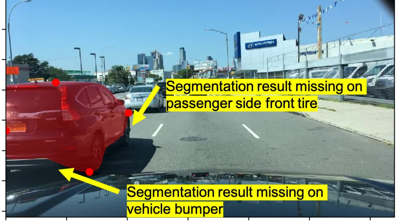
In 2019, we released an ML-powered interactive labeling tool called Auto-segment for Ground Truth that allows you to quickly and easily create high-quality segmentation masks. For more information, see Auto-Segmentation Tool. This feature works by allowing you to click the top-, left-, bottom-, and right-most “extreme points” on an object. An ML model running in the background will ingest this user input and return a high-quality segmentation mask that immediately renders in the Ground Truth labeling tool. However, this feature only allows you to place four clicks. In certain cases, the ML-generated mask may inadvertently miss certain portions of an image, such as around the object boundary where edges are indistinct or where color, saturation, or shadows blend into the surroundings.
Extreme point clicking with a flexible number of corrective clicks
We now have enhanced the tool to allow extra clicks of boundary points, which provides real-time feedback to the ML model. This allows you to create a more accurate segmentation mask. In the following example, the initial segmentation result isn’t accurate because of the weak boundaries near the shadow. Importantly, this tool operates in a mode that allows for real-time feedback—it doesn’t require you to specify all points at once. Instead, you can first make four mouse clicks, which will trigger the ML model to produce a segmentation mask. Then you can inspect this mask, locate any potential inaccuracies, and subsequently place additional clicks as appropriate to “nudge” the model into the correct result.
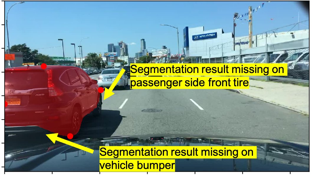
Our previous labeling tool allowed you to place exactly four mouse clicks (red dots). The initial segmentation result (shaded red area) isn’t accurate because of the weak boundaries near the shadow (bottom-left of red mask).
With our enhanced labeling tool, the user again first makes four mouse clicks (red dots in top figure). Then you have the opportunity to inspect the resulting segmentation mask (shaded red area in top figure). You can make additional mouse clicks (green dots in bottom figure) to cause the model to refine the mask (shaded red area in bottom figure).
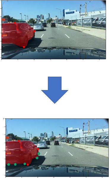
Compared with the original version of the tool, the enhanced version provides an improved result when objects are deformable, non-convex, and vary in shape and appearance.
We simulated the performance of this improved tool on sample data by first running the baseline tool (with only four extreme clicks) to generate a segmentation mask and evaluated its mean Intersection over Union (mIoU), a common measure of accuracy for segmentation masks. Then we applied simulated corrective clicks and evaluated the improvement in mIoU after each simulated click. The following table summarizes these results. The first row shows the mIoU, and the second row shows the error (which is given by 100% minus the mIoU). With only five additional mouse clicks, we can reduce the error by 9% for this task!
| . | . | Number of Corrective Clicks | . | |||
| . | Baseline | 1 | 2 | 3 | 4 | 5 |
| mIoU | 72.72 | 76.56 | 77.62 | 78.89 | 80.57 | 81.73 |
| Error | 27% | 23% | 22% | 21% | 19% | 18% |
Integration with Ground Truth and performance profiling
To integrate this model with Ground Truth, we follow a standard architecture pattern as shown in the following diagram. First, we build the ML model into a Docker image and deploy it to Amazon Elastic Container Registry (Amazon ECR), a fully managed Docker container registry that makes it easy to store, share, and deploy container images. Using the SageMaker Inference Toolkit in building the Docker image allows us to easily use best practices for model serving and achieve low-latency inference. We then create an Amazon SageMaker real-time endpoint to host the model. We introduce an AWS Lambda function as a proxy in front of the SageMaker endpoint to offer various types of data transformation. Finally, we use Amazon API Gateway as a way of integrating with our front end, the Ground Truth labeling application, to provide secure authentication to our backend.

You can follow this generic pattern for your own use cases for purpose-built ML tools and to integrate them with custom Ground Truth task UIs. For more information, refer to Build a custom data labeling workflow with Amazon SageMaker Ground Truth.
After provisioning this architecture and deploying our model using the AWS Cloud Development Kit (AWS CDK), we evaluated the latency characteristics of our model with different SageMaker instance types. This is very straightforward to do because we use SageMaker real-time inference endpoints to serve our model. SageMaker real-time inference endpoints integrate seamlessly with Amazon CloudWatch and emit such metrics as memory utilization and model latency with no required setup (see SageMaker Endpoint Invocation Metrics for more details).
In the following figure, we show the ModelLatency metric natively emitted by SageMaker real-time inference endpoints. We can easily use various metric math functions in CloudWatch to show latency percentiles, such as p50 or p90 latency.
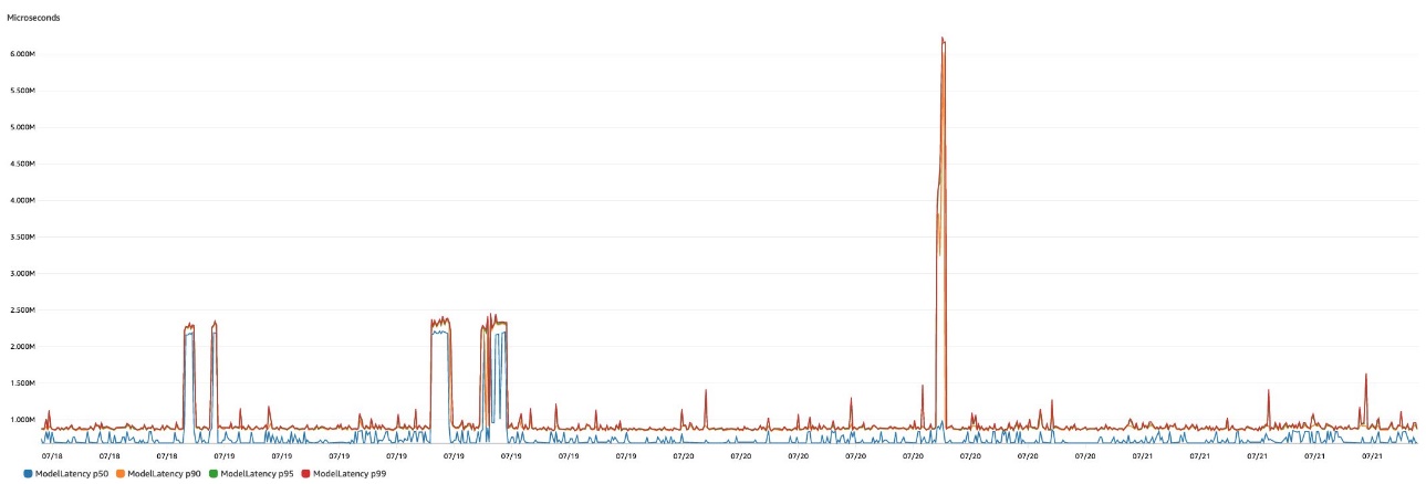
The following table summarizes these results for our enhanced extreme clicking tool for semantic segmentation for three instance types: p2.xlarge, p3.2xlarge, and g4dn.xlarge. Although the p3.2xlarge instance provides the lowest latency, the g4dn.xlarge instance provides the best cost-to-performance ratio. The g4dn.xlarge instance is only 8% slower (35 milliseconds) than the p3.2xlarge instance, but it is 81% less expensive on an hourly basis than the p3.2xlarge (see Amazon SageMaker Pricing for more details on SageMaker instance types and pricing).
| SageMaker Instance Type | p90 Latency (ms) | |
| 1 | p2.xlarge | 751 |
| 2 | p3.2xlarge | 424 |
| 3 | g4dn.xlarge | 459 |
Conclusion
In this post, we introduced an extension to the Ground Truth auto segment feature for semantic segmentation annotation tasks. Whereas the original version of the tool allows you to make exactly four mouse clicks, which triggers a model to provide a high-quality segmentation mask, the extension enables you to make corrective clicks and thereby update and guide the ML model to make better predictions. We also presented a basic architectural pattern that you can use to deploy and integrate interactive tools into Ground Truth labeling UIs. Finally, we summarized the model latency, and showed how the use of SageMaker real-time inference endpoints makes it easy to monitor model performance.
To learn more about how this tool can reduce labeling cost and increase accuracy, visit Amazon SageMaker Data Labeling to start a consultation today.
About the authors
 Jonathan Buck is a Software Engineer at Amazon Web Services working at the intersection of machine learning and distributed systems. His work involves productionizing machine learning models and developing novel software applications powered by machine learning to put the latest capabilities in the hands of customers.
 Li Erran Li is the applied science manager at humain-in-the-loop services, AWS AI, Amazon. His research interests are 3D deep learning, and vision and language representation learning. Previously he was a senior scientist at Alexa AI, the head of machine learning at Scale AI and the chief scientist at Pony.ai. Before that, he was with the perception team at Uber ATG and the machine learning platform team at Uber working on machine learning for autonomous driving, machine learning systems and strategic initiatives of AI. He started his career at Bell Labs and was adjunct professor at Columbia University. He co-taught tutorials at ICML’17 and ICCV’19, and co-organized several workshops at NeurIPS, ICML, CVPR, ICCV on machine learning for autonomous driving, 3D vision and robotics, machine learning systems and adversarial machine learning. He has a PhD in computer science at Cornell University. He is an ACM Fellow and IEEE Fellow.
What Are Foundation Models?
The mics were live and tape was rolling in the studio where the Miles Davis Quintet was recording dozens of tunes in 1956 for Prestige Records.
When an engineer asked for the next song’s title, Davis shot back, “I’ll play it, and tell you what it is later.”
Like the prolific jazz trumpeter and composer, researchers have been generating AI models at a feverish pace, exploring new architectures and use cases. Focused on plowing new ground, they sometimes leave to others the job of categorizing their work.
A team of more than a hundred Stanford researchers collaborated to do just that in a 214-page paper released in the summer of 2021.
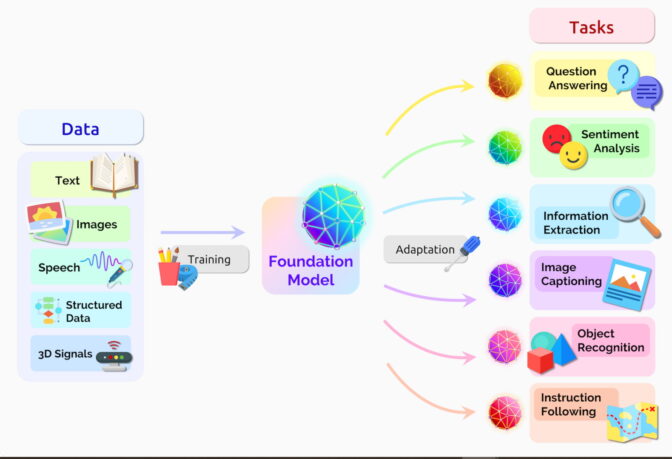
They said transformer models, large language models (LLMs) and other neural networks still being built are part of an important new category they dubbed foundation models.
Foundation Models Defined
A foundation model is an AI neural network — trained on mountains of raw data, generally with unsupervised learning — that can be adapted to accomplish a broad range of tasks, the paper said.
“The sheer scale and scope of foundation models from the last few years have stretched our imagination of what’s possible,” they wrote.
Two important concepts help define this umbrella category: Data gathering is easier, and opportunities are as wide as the horizon.
No Labels, Lots of Opportunity
Foundation models generally learn from unlabeled datasets, saving the time and expense of manually describing each item in massive collections.
Earlier neural networks were narrowly tuned for specific tasks. With a little fine-tuning, foundation models can handle jobs from translating text to analyzing medical images.
Foundation models are demonstrating “impressive behavior,” and they’re being deployed at scale, the group said on the website of its research center formed to study them. So far, they’ve posted more than 50 papers on foundation models from in-house researchers alone.
“I think we’ve uncovered a very small fraction of the capabilities of existing foundation models, let alone future ones,” said Percy Liang, the center’s director, in the opening talk of the first workshop on foundation models.
AI’s Emergence and Homogenization
In that talk, Liang coined two terms to describe foundation models:
Emergence refers to AI features still being discovered, such as the many nascent skills in foundation models. He calls the blending of AI algorithms and model architectures homogenization, a trend that helped form foundation models. (See chart below.)
 The field continues to move fast.
A year after the group defined foundation models, other tech watchers coined a related term — generative AI. It’s an umbrella term for transformers, large language models, diffusion models and other neural networks capturing people’s imaginations because they can create text, images, music, software and more.
Generative AI has the potential to yield trillions of dollars of economic value, said executives from the venture firm Sequoia Capital who shared their views in a recent AI Podcast.
A Brief History of Foundation Models
“We are in a time where simple methods like neural networks are giving us an explosion of new capabilities,” said Ashish Vaswani, an entrepreneur and former senior staff research scientist at Google Brain who led work on the seminal 2017 paper on transformers.
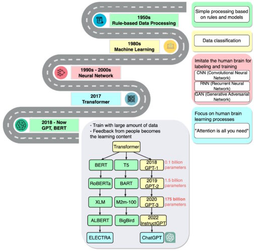
That work inspired researchers who created BERT and other large language models, making 2018 “a watershed moment” for natural language processing, a report on AI said at the end of that year.
Google released BERT as open-source software, spawning a family of follow-ons and setting off a race to build ever larger, more powerful LLMs. Then it applied the technology to its search engine so users could ask questions in simple sentences.
In 2020, researchers at OpenAI announced another landmark transformer, GPT-3. Within weeks, people were using it to create poems, programs, songs, websites and more.
“Language models have a wide range of beneficial applications for society,” the researchers wrote.
Their work also showed how large and compute-intensive these models can be. GPT-3 was trained on a dataset with nearly a trillion words, and it sports a whopping 175 billion parameters, a key measure of the power and complexity of neural networks.
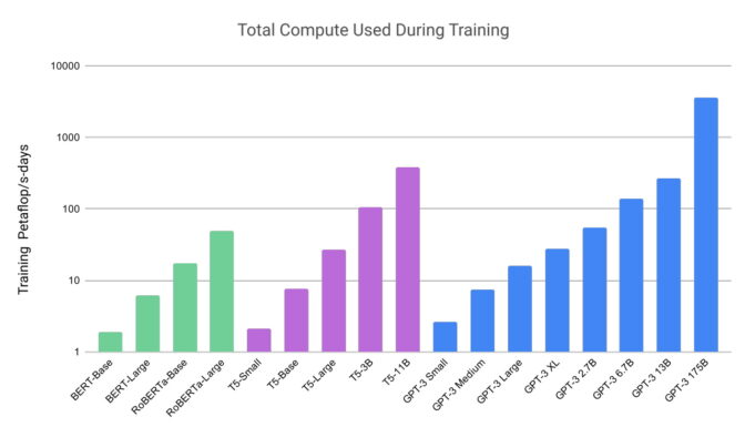
“I just remember being kind of blown away by the things that it could do,” said Liang, speaking of GPT-3 in a podcast.
The latest iteration, ChatGPT — trained on 10,000 NVIDIA GPUs — is even more engaging, attracting over 100 million users in just two months. Its release has been called the iPhone moment for AI because it helped so many people see how they could use the technology.
From Text to Images
About the same time ChatGPT debuted, another class of neural networks, called diffusion models, made a splash. Their ability to turn text descriptions into artistic images attracted casual users to create amazing images that went viral on social media.
The first paper to describe a diffusion model arrived with little fanfare in 2015. But like transformers, the new technique soon caught fire.
Researchers posted more than 200 papers on diffusion models last year, according to a list maintained by James Thornton, an AI researcher at the University of Oxford.
In a tweet, Midjourney CEO David Holz revealed that his diffusion-based, text-to-image service has more than 4.4 million users. Serving them requires more than 10,000 NVIDIA GPUs mainly for AI inference, he said in an interview (subscription required).
Dozens of Models in Use
Hundreds of foundation models are now available. One paper catalogs and classifies more than 50 major transformer models alone (see chart below).
The Stanford group benchmarked 30 foundation models, noting the field is moving so fast they did not review some new and prominent ones.
Startup NLP Cloud, a member of the NVIDIA Inception program that nurtures cutting-edge startups, says it uses about 25 large language models in a commercial offering that serves airlines, pharmacies and other users. Experts expect that a growing share of the models will be made open source on sites like Hugging Face’s model hub.
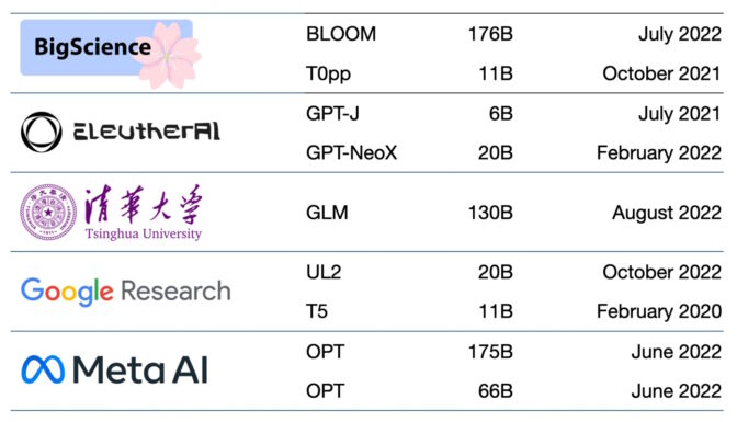
Foundation models keep getting larger and more complex, too.
That’s why — rather than building new models from scratch — many businesses are already customizing pretrained foundation models to turbocharge their journeys into AI.
Foundations in the Cloud
One venture capital firm lists 33 use cases for generative AI, from ad generation to semantic search.
Major cloud services have been using foundation models for some time. For example, Microsoft Azure worked with NVIDIA to implement a transformer for its Translator service. It helped disaster workers understand Haitian Creole while they were responding to a 7.0 earthquake.
In February, Microsoft announced plans to enhance its browser and search engine with ChatGPT and related innovations. “We think of these tools as an AI copilot for the web,” the announcement said.
Google announced Bard, an experimental conversational AI service. It plans to plug many of its products into the power of its foundation models like LaMDA, PaLM, Imagen and MusicLM.
“AI is the most profound technology we are working on today,” the company’s blog wrote.
Startups Get Traction, Too
Startup Jasper expects to log $75 million in annual revenue from products that write copy for companies like VMware. It’s leading a field of more than a dozen companies that generate text, including Writer, an NVIDIA Inception member.
Other Inception members in the field include Tokyo-based rinna that’s created chatbots used by millions in Japan. In Tel Aviv, Tabnine runs a generative AI service that’s automated up to 30% of the code written by a million developers globally.
A Platform for Healthcare
Researchers at startup Evozyne used foundation models in NVIDIA BioNeMo to generate two new proteins. One could treat a rare disease and another could help capture carbon in the atmosphere.

BioNeMo, a software platform and cloud service for generative AI in drug discovery, offers tools to train, run inference and deploy custom biomolecular AI models. It includes MegaMolBART, a generative AI model for chemistry developed by NVIDIA and AstraZeneca.
“Just as AI language models can learn the relationships between words in a sentence, our aim is that neural networks trained on molecular structure data will be able to learn the relationships between atoms in real-world molecules,” said Ola Engkvist, head of molecular AI, discovery sciences and R&D at AstraZeneca, when the work was announced.
Separately, the University of Florida’s academic health center collaborated with NVIDIA researchers to create GatorTron. The large language model aims to extract insights from massive volumes of clinical data to accelerate medical research.
A Stanford center is applying the latest diffusion models to advance medical imaging. NVIDIA also helps healthcare companies and hospitals use AI in medical imaging, speeding diagnosis of deadly diseases.
AI Foundations for Business
Another new framework, NVIDIA NeMo Megatron, aims to let any business create its own billion- or trillion-parameter transformers to power custom chatbots, personal assistants and other AI applications.
It created the 530-parameter Megatron-Turing Natural Language Generation model (MT-NLG) that powers TJ, the Toy Jensen avatar that gave part of the keynote at NVIDIA GTC last year.
Foundation models — connected to 3D platforms like NVIDIA Omniverse — will be key to simplifying development of the metaverse, the 3D evolution of the internet. These models will power applications and assets for entertainment and industrial users.
Factories and warehouses are already applying foundation models inside digital twins, realistic simulations that help find more efficient ways to work.
Foundation models can ease the job of training autonomous vehicles and robots that assist humans on factory floors and logistics centers like the one described below.
New uses for foundation models are emerging daily, as are challenges in applying them.
Several papers on foundation and generative AI models describing risks such as:
- amplifying bias implicit in the massive datasets used to train models,
- introducing inaccurate or misleading information in images or videos, and
- violating intellectual property rights of existing works.
“Given that future AI systems will likely rely heavily on foundation models, it is imperative that we, as a community, come together to develop more rigorous principles for foundation models and guidance for their responsible development and deployment,” said the Stanford paper on foundation models.
Current ideas for safeguards include filtering prompts and their outputs, recalibrating models on the fly and scrubbing massive datasets.
“These are issues we’re working on as a research community,” said Bryan Catanzaro, vice president of applied deep learning research at NVIDIA. “For these models to be truly widely deployed, we have to invest a lot in safety.”
It’s one more field AI researchers and developers are plowing as they create the future.
New Library Updates in PyTorch 2.0
Summary
We are bringing a number of improvements to the current PyTorch libraries, alongside the PyTorch 2.0 release. These updates demonstrate our focus on developing common and extensible APIs across all domains to make it easier for our community to build ecosystem projects on PyTorch.
Along with 2.0, we are also releasing a series of beta updates to the PyTorch domain libraries, including those that are in-tree, and separate libraries including TorchAudio, TorchVision, and TorchText. An update for TorchX is also being released as it moves to community supported mode. Please find the list of the latest stable versions and updates below.
Latest Stable Library Versions (Full List)
| TorchArrow 0.1.0 | TorchRec 0.4.0 | TorchVision 0.15 |
| TorchAudio 2.0 | TorchServe 0.7.1 | TorchX 0.4.0 |
| TorchData 0.6.0 | TorchText 0.15.0 | PyTorch on XLA Devices 1.14 |
*To see prior versions or (unstable) nightlies, click on versions in the top left menu above ‘Search Docs’.
TorchAudio
[Beta] Data augmentation operators
The release adds several data augmentation operators under torchaudio.functional and torchaudio.transforms:
- torchaudio.functional.add_noise
- torchaudio.functional.convolve
- torchaudio.functional.deemphasis
- torchaudio.functional.fftconvolve
- torchaudio.functional.preemphasis
- torchaudio.functional.speed
- torchaudio.transforms.AddNoise
- torchaudio.transforms.Convolve
- torchaudio.transforms.Deemphasis
- torchaudio.transforms.FFTConvolve
- torchaudio.transforms.Preemphasis
- torchaudio.transforms.Speed
- torchaudio.transforms.SpeedPerturbation
The operators can be used to synthetically diversify training data to improve the generalizability of downstream models.
For usage details, please refer to the functional and transform documentation and Audio Data Augmentation tutorial.
[Beta] WavLM and XLS-R models
The release adds two self-supervised learning models for speech and audio.
Besides the model architectures, torchaudio also supports corresponding pre-trained pipelines:
- torchaudio.pipelines.WAVLM_BASE
- torchaudio.pipelines.WAVLM_BASE_PLUS
- torchaudio.pipelines.WAVLM_LARGE
- torchaudio.pipelines.WAV2VEC_XLSR_300M
- torchaudio.pipelines.WAV2VEC_XLSR_1B
- torchaudio.pipelines.WAV2VEC_XLSR_2B
For usage details, please refer to the factory function and pre-trained pipelines documentation.
TorchRL
The initial release of torchrl includes several features that span across the entire RL domain. TorchRL can already be used in online, offline, multi-agent, multi-task and distributed RL settings, among others. See below:
[Beta] Environment wrappers and transforms
torchrl.envs includes several wrappers around common environment libraries. This allows users to swap one library with another without effort. These wrappers build an interface between these simulators and torchrl:
- dm_control:
- Gym
- Brax
- EnvPool
- Jumanji
- Habitat
It also comes with many commonly used transforms and vectorized environment utilities that allow for a fast execution across simulation libraries. Please refer to the documentation for more detail.
[Beta] Datacollectors
Data collection in RL is made easy via the usage of single process or multiprocessed/distributed data collectors that execute the policy in the environment over a desired duration and deliver samples according to the user’s needs. These can be found in torchrl.collectors and are documented here.
[Beta] Objective modules
Several objective functions are included in torchrl.objectives, among which:
- A generic PPOLoss class and derived ClipPPOLoss and KLPPOLoss
- SACLoss and DiscreteSACLoss
- DDPGLoss
- DQNLoss
- REDQLoss
- A2CLoss
- TD3Loss
- ReinforceLoss
- Dreamer
Vectorized value function operators also appear in the library. Check the documentation here.
[Beta] Models and exploration strategies
We provide multiple models, modules and exploration strategies. Get a detailed description in the doc.
[Beta] Composable replay buffer
A composable replay buffer class is provided that can be used to store data in multiple contexts including single and multi-agent, on and off-policy and many more.. Components include:
- Storages (list, physical or memory-based contiguous storages)
- Samplers (Prioritized, sampler without repetition)
- Writers
- Possibility to add transforms
Replay buffers and other data utilities are documented here.
[Beta] Logging tools and trainer
We support multiple logging tools including tensorboard, wandb and mlflow.
We provide a generic Trainer class that allows for easy code recycling and checkpointing.
These features are documented here.
TensorDict
TensorDict is a new data carrier for PyTorch.
[Beta] TensorDict: specialized dictionary for PyTorch
TensorDict allows you to execute many common operations across batches of tensors carried by a single container. TensorDict supports many shape and device or storage operations, and can readily be used in distributed settings. Check the documentation to know more.
[Beta] @tensorclass: a dataclass for PyTorch
Like TensorDict, tensorclass provides the opportunity to write dataclasses with built-in torch features such as shape or device operations.
[Beta] tensordict.nn: specialized modules for TensorDict
The tensordict.nn module provides specialized nn.Module subclasses that make it easy to build arbitrarily complex graphs that can be executed with TensorDict inputs. It is compatible with the latest PyTorch features such as functorch, torch.fx and torch.compile.
TorchRec
[Beta] KeyedJaggedTensor All-to-All Redesign and Input Dist Fusion
We observed performance regression due to a bottleneck in sparse data distribution for models that have multiple, large KJTs to redistribute.
To combat this we altered the comms pattern to transport the minimum data required in the initial collective to support the collective calls for the actual KJT tensor data. This data sent in the initial collective, ‘splits’ means more data is transmitted over the comms stream overall, but the CPU is blocked for significantly shorter amounts of time leading to better overall QPS.
Furthermore, we altered the TorchRec train pipeline to group the initial collective calls for the splits together before launching the more expensive KJT tensor collective calls. This fusion minimizes the CPU blocked time as launching each subsequent input distribution is no longer dependent on the previous input distribution.
With this feature, variable batch sizes are now natively supported across ranks. These features are documented here.
TorchVision
[Beta] Extending TorchVision’s Transforms to Object Detection, Segmentation & Video tasks
TorchVision is extending its Transforms API! Here is what’s new:
- You can use them not only for Image Classification but also for Object Detection, Instance & Semantic Segmentation and Video Classification.
- You can use new functional transforms for transforming Videos, Bounding Boxes and Segmentation Masks.
Learn more about these new transforms from our docs, and submit any feedback in our dedicated issue.
TorchText
[Beta] Adding scriptable T5 and Flan-T5 to the TorchText library with incremental decoding support!
TorchText has added the T5 model architecture with pre-trained weights for both the original T5 paper and Flan-T5. The model is fully torchscriptable and features an optimized multiheaded attention implementation. We include several examples of how to utilize the model including summarization, classification, and translation.
For more details, please refer to our docs.
TorchX
TorchX is moving to community supported mode. More details will be coming in at a later time.
PyTorch 2.0: Our next generation release that is faster, more Pythonic and Dynamic as ever
We are excited to announce the release of PyTorch® 2.0 which we highlighted during the PyTorch Conference on 12/2/22! PyTorch 2.0 offers the same eager-mode development and user experience, while fundamentally changing and supercharging how PyTorch operates at compiler level under the hood with faster performance and support for Dynamic Shapes and Distributed.
This next-generation release includes a Stable version of Accelerated Transformers (formerly called Better Transformers); Beta includes torch.compile as the main API for PyTorch 2.0, the scaled_dot_product_attention function as part of torch.nn.functional, the MPS backend, functorch APIs in the torch.func module; and other Beta/Prototype improvements across various inferences, performance and training optimization features on GPUs and CPUs. For a comprehensive introduction and technical overview of torch.compile, please visit the 2.0 Get Started page.
Along with 2.0, we are also releasing a series of beta updates to the PyTorch domain libraries, including those that are in-tree, and separate libraries including TorchAudio, TorchVision, and TorchText. An update for TorchX is also being released as it moves to community supported mode. More details can be found in this library blog.
This release is composed of over 4,541 commits and 428 contributors since 1.13.1. We want to sincerely thank our dedicated community for your contributions. As always, we encourage you to try these out and report any issues as we improve 2.0 and the overall 2-series this year.
Summary:
- torch.compile is the main API for PyTorch 2.0, which wraps your model and returns a compiled model. It is a fully additive (and optional) feature and hence 2.0 is 100% backward compatible by definition.
- As an underpinning technology of torch.compile, TorchInductor with Nvidia and AMD GPUs will rely on OpenAI Triton deep learning compiler to generate performant code and hide low level hardware details. OpenAI Triton-generated kernels achieve performance that’s on par with hand-written kernels and specialized cuda libraries such as cublas.
- Accelerated Transformers introduce high-performance support for training and inference using a custom kernel architecture for scaled dot product attention (SPDA). The API is integrated with torch.compile() and model developers may also use the scaled dot product attention kernels directly by calling the new scaled_dot_product_attention() operator.
- Metal Performance Shaders (MPS) backend provides GPU accelerated PyTorch training on Mac platforms with added support for Top 60 most used ops, bringing coverage to over 300 operators.
- Amazon AWS optimizes the PyTorch CPU inference on AWS Graviton3 based C7g instances. PyTorch 2.0 improves inference performance on Graviton compared to the previous releases, including improvements for Resnet50 and Bert.
- New prototype features and technologies across TensorParallel, DTensor, 2D parallel, TorchDynamo, AOTAutograd, PrimTorch and TorchInductor.
| Stable | Beta | Prototype | Performance Improvements |
| Dispatchable Collectives | |||
| Torch.set_default & torch.device | |||
*To see a full list of public 2.0, 1.13 and 1.12 feature submissions click here.
Stable Features
[Stable] Accelerated PyTorch 2 Transformers (previously known as “Better Transformer”)
The PyTorch 2.0 release includes a new high-performance implementation of the PyTorch Transformer API, formerly known as “Better Transformer API, “ now renamed Accelerated PyTorch 2 Transformers. In releasing accelerated PT2 Transformers, our goal is to make training and deployment of state-of-the-art Transformer models affordable across the industry. This release introduces high-performance support for training and inference using a custom kernel architecture for scaled dot product attention (SPDA).
Similar to the “fastpath” architecture, custom kernels are fully integrated into the PyTorch Transformer API – thus, using the native Transformer and MultiHeadAttention API will enable users to:
- transparently see significant speed improvements;
- support many more use cases including models using Cross-Attention, Transformer Decoders, and for training models; and
- continue to use fastpath inference for fixed and variable sequence length Transformer Encoder and Self Attention use cases.
To take full advantage of different hardware models and Transformer use cases, multiple SDPA custom kernels are supported (see below), with custom kernel selection logic that will pick the highest-performance kernel for a given model and hardware type. In addition to the existing Transformer API, model developers may also use the
scaled dot product attention kernels directly by calling the new scaled_dot_product_attention() operator. Accelerated PyTorch 2 Transformers are integrated with torch.compile() . To use your model while benefiting from the additional acceleration of PT2-compilation (for inference or training), pre-process the model with model = torch.compile(model).
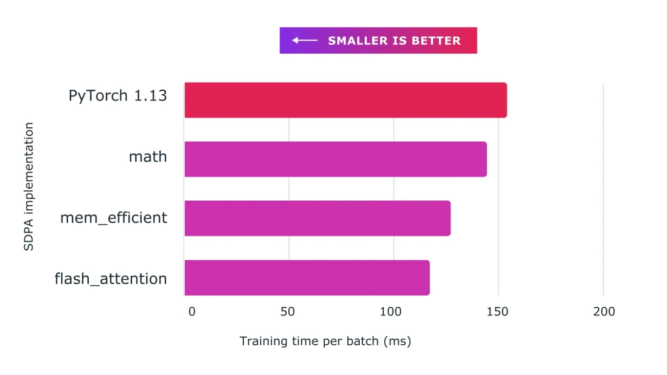
We have achieved major speedups for training transformer models and in particular large language models with Accelerated PyTorch 2 Transformers using a combination of custom kernels and torch.compile().
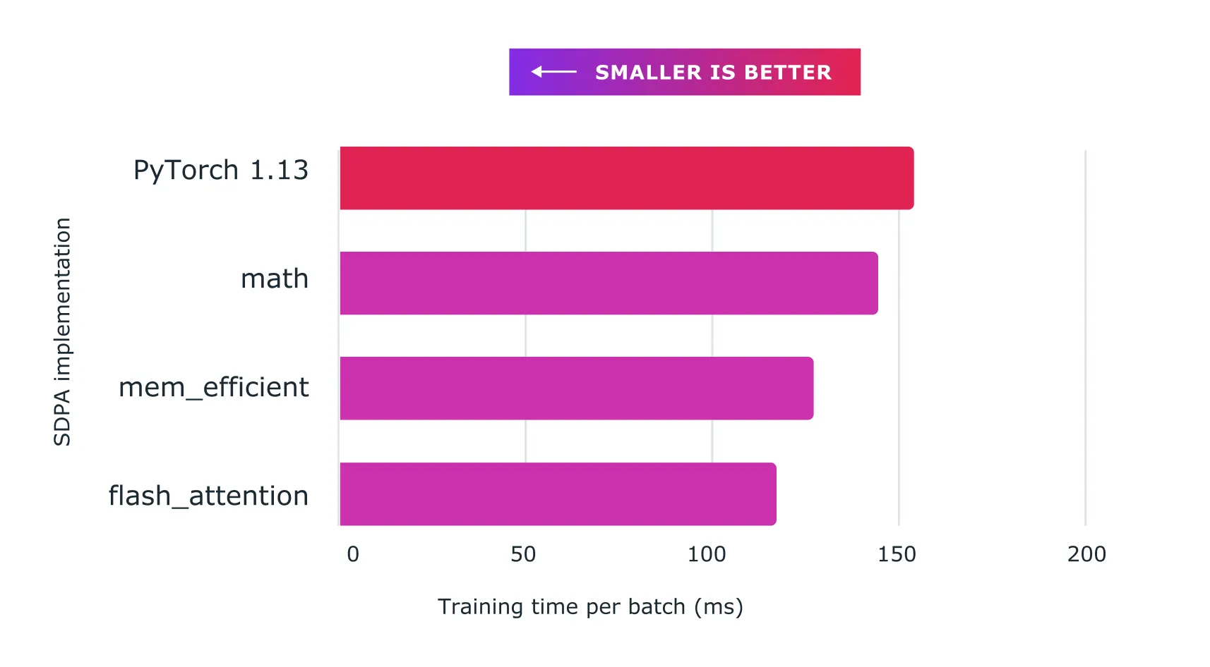 Figure: Using scaled dot product attention with custom kernels and torch.compile delivers significant speedups for training large language models, such as for nanoGPT shown here.
Beta Features
[Beta] torch.compile
torch.compile is the main API for PyTorch 2.0, which wraps your model and returns a compiled model. It is a fully additive (and optional) feature and hence 2.0 is 100% backward compatible by definition.
Underpinning torch.compile are new technologies – TorchDynamo, AOTAutograd, PrimTorch and TorchInductor:
- TorchDynamo captures PyTorch programs safely using Python Frame Evaluation Hooks and is a significant innovation that was a result of 5 years of our R&D into safe graph capture.
- AOTAutograd overloads PyTorch’s autograd engine as a tracing autodiff for generating ahead-of-time backward traces.
- PrimTorch canonicalizes ~2000+ PyTorch operators down to a closed set of ~250 primitive operators that developers can target to build a complete PyTorch backend. This substantially lowers the barrier of writing a PyTorch feature or backend.
- TorchInductor is a deep learning compiler that generates fast code for multiple accelerators and backends. For NVIDIA and AMD GPUs, it uses OpenAI Triton as a key building block. For intel CPUs, we generate C++ code using multithreading, vectorized instructions and offloading appropriate operations to mkldnn when possible.
With all the new technologies, torch.compile is able to work 93% of time across 165 open-source models and runs 20% faster on average at float32 precision and 36% faster on average at AMP precision.
For more information, please refer to https://pytorch.org/get-started/pytorch-2.0/ and for TorchInductor CPU with Intel here.
[Beta] PyTorch MPS Backend
MPS backend provides GPU-accelerated PyTorch training on Mac platforms. This release brings improved correctness, stability, and operator coverage.
MPS backend now includes support for the Top 60 most used ops, along with the most frequently requested operations by the community, bringing coverage to over 300 operators. The major focus of the release was to enable full OpInfo-based forward and gradient mode testing to address silent correctness issues. These changes have resulted in wider adoption of MPS backend by 3rd party networks such as Stable Diffusion, YoloV5, WhisperAI, along with increased coverage for Torchbench networks and Basic tutorials. We encourage developers to update to the latest macOS release to see the best performance and stability on the MPS backend.
Links
- MPS Backend
- Developer information
- Accelerated PyTorch training on Mac
- Metal, Metal Performance Shaders & Metal Performance Shaders Graph
[Beta] Scaled dot product attention 2.0
We are thrilled to announce the release of PyTorch 2.0, which introduces a powerful scaled dot product attention function as part of torch.nn.functional. This function includes multiple implementations that can be seamlessly applied depending on the input and hardware in use.
In previous versions of PyTorch, you had to rely on third-party implementations and install separate packages to take advantage of memory-optimized algorithms like FlashAttention. With PyTorch 2.0, all these implementations are readily available by default.
These implementations include FlashAttention from HazyResearch, Memory-Efficient Attention from the xFormers project, and a native C++ implementation that is ideal for non-CUDA devices or when high-precision is required.
PyTorch 2.0 will automatically select the optimal implementation for your use case, but you can also toggle them individually for finer-grained control. Additionally, the scaled dot product attention function can be used to build common transformer architecture components.
Learn more with the documentation and this tutorial.
[Beta] functorch -> torch.func
Inspired by Google JAX, functorch is a library that offers composable vmap (vectorization) and autodiff transforms. It enables advanced autodiff use cases that would otherwise be tricky to express in PyTorch. Examples include:
- model ensembling
- efficiently computing jacobians and hessians
- computing per-sample-gradients (or other per-sample quantities)
We’re excited to announce that, as the final step of upstreaming and integrating functorch into PyTorch, the functorch APIs are now available in the torch.func module. Our function transform APIs are identical to before, but we have changed how the interaction with NN modules work. Please see the docs and the migration guide for more details.
Furthermore, we have added support for torch.autograd.Function: one is now able to apply function transformations (e.g. vmap, grad, jvp) over torch.autograd.Function.
[Beta] Dispatchable Collectives
Dispatchable collectives is an improvement to the existing init_process_group() API which changes backend to an optional argument. For users, the main advantage of this feature is that it will allow them to write code that can run on both GPU and CPU machines without having to change the backend specification. The dispatchability feature will also make it easier for users to support both GPU and CPU collectives, as they will no longer need to specify the backend manually (e.g. “NCCL” or “GLOO”). Existing backend specifications by users will be honored and will not require change.
Usage example:
import torch.distributed.dist
…
# old
dist.init_process_group(backend=”nccl”, ...)
dist.all_reduce(...) # with CUDA tensors works
dist.all_reduce(...) # with CPU tensors does not work

# new
dist.init_process_group(...) # backend is optional
dist.all_reduce(...) # with CUDA tensors works
dist.all_reduce(...) # with CPU tensors works
Learn more here.
[Beta] torch.set_default_device and torch.device as context manager
torch.set_default_device allows users to change the default device that factory functions in PyTorch allocate on. For example, if you torch.set_default_device(‘cuda’), a call to torch.empty(2) will allocate on CUDA (rather than on CPU). You can also use torch.device as a context manager to change the default device on a local basis. This resolves a long standing feature request from PyTorch’s initial release for a way to do this.
Learn more here.
[Beta] “X86” as the new default quantization backend for x86 CPU
The new X86 quantization backend, which utilizes FBGEMM and oneDNN kernel libraries, replaces FBGEMM as the default quantization backend for x86 CPU platforms and offers improved int8 inference performance compared to the original FBGEMM backend, leveraging the strengths of both libraries, with 1.3X – 2X inference performance speedup measured on 40+ deep learning models. The new backend is functionally compatible with the original FBGEMM backend.
Table: Geomean Speedup of X86 Quantization Backend vs. FBGEMM Backend
| 1 core/instance | 2 cores/instance | 4 cores/instance | 1 socket (32 cores)/instance | |
| Intel(R) Xeon(R) Platinum 8358 CPU @ 2.60GHz | 1.76X | 1.80X | 2.04X | 1.34X |
By default, users on x86 platforms will utilize the x86 quantization backend and their PyTorch programs will remain unchanged when using the default backend. Alternatively, users have the option to specify “X86” as the quantization backend explicitly. Example code is show below:
import torch
from torch.ao.quantization import get_default_qconfig_mappingfrom torch.quantization.quantize_fx
import prepare_fx, convert_fx

# get default configuration
qconfig_mapping = get_default_qconfig_mapping()

# or explicitly specify the backend
# qengine = 'x86'
# torch.backends.quantized.engine = qengine
# qconfig_mapping = get_default_qconfig_mapping(qengine)

# construct fp32 model
model_fp32 = ...

# prepare
prepared_model = prepare_fx(model_fp32, qconfig_mapping, example_inputs=x)

# calibrate
...

# convert
quantized_model = convert_fx(prepared_model)
Find more information: https://github.com/pytorch/pytorch/issues/83888 and https://www.intel.com/content/www/us/en/developer/articles/technical/accelerate-pytorch-int8-inf-with-new-x86-backend.html.
[Beta] GNN inference and training optimization on CPU
PyTorch 2.0 includes several critical optimizations to improve GNN inference and training performance on CPU. Before 2.0, GNN models of PyG suffers from low efficiency on CPU due to lack of performance tuning for several critical kernels (scatter/gather, etc) and the lack of GNN-related sparse matrix multiplication ops. To be specific, optimizations include:
- scatter_reduce: performance hotspot in Message Passing when the edge index is stored in Coordinate format (COO).
- gather: backward of scatter_reduce, specially tuned for the GNN compute when the index is an expanded tensor.
- torch.sparse.mm with reduce flag: performance hotspot in Message Passing when the edge index is stored in Compressed Sparse Row (CSR). Supported reduce flag of: sum, mean, amax, amin.
On PyG benchmarks/examples, OGB benchmarks, a 1.12x – 4.07x performance speedup is measured (1.13.1 compared with 2.0) for single node inference and training.
| Model-Dataset | Option | Speedup Ratio |
| GCN-Reddit (inference) | 512-2-64-dense | 1.22x |
| 1024-3-128-dense | 1.25x | |
| 512-2-64-sparse | 1.31x | |
| 1024-3-128-sparse | 1.68x | |
| 512-2-64-dense | 1.22x | |
| GraphSage-ogbn-products (inference) | 1024-3-128-dense | 1.15x |
| 512-2-64-sparse | 1.20x | |
| 1024-3-128-sparse | 1.33x | |
| full-batch-sparse | 4.07x | |
| GCN-PROTEINS (training) | 3-32 | 1.67x |
| GCN-REDDIT-BINARY (training) | 3-32 | 1.67x |
| GCN-Reddit (training) | 512-2-64-dense | 1.20x |
| 1024-3-128-dense | 1.12x |
Learn more: PyG CPU Performance Optimization.
[Beta] Accelerating inference on CPU with PyTorch by leveraging oneDNN Graph
oneDNN Graph API extends oneDNN with a flexible graph API to maximize the optimization opportunity for generating efficient code on AI hardware.
- It automatically identifies the graph partitions to be accelerated via fusion.
- The fusion patterns focus on fusing compute-intensive operations such as convolution, matmul and their neighbor operations for both inference and training use cases.
- Although work is ongoing to integrate oneDNN Graph with TorchDynamo as well, its integration with the PyTorch JIT Fuser attained beta status in PyTorch 2.0 for Float32 & BFloat16 inference (on machines that support AVX512_BF16 ISA).
From a developer’s/researcher’s perspective, the usage is quite simple & intuitive, with the only change in code being an API invocation:
- Leverage oneDNN Graph, with JIT-tracing, a model is profiled with an example input.
- The context manager with torch.jit.fuser(“fuser3”): can also be used instead of invoking torch.jit.enable_onednn_fusion(True).
- For accelerating BFloat16 inference, we rely on eager-mode AMP (Automatic Mixed Precision) support in PyTorch & disable JIT mode’s AMP, as both of them are currently divergent:
# Assuming we have a model of the name 'model'

example_input = torch.rand(1, 3, 224, 224)

# enable oneDNN Graph
torch.jit.enable_onednn_fusion(True)
# Disable AMP for JIT
torch._C._jit_set_autocast_mode(False)
with torch.no_grad(), torch.cpu.amp.autocast():
	model = torch.jit.trace(model, (example_input))
	model = torch.jit.freeze(model)
 	# 2 warm-ups (2 for tracing/scripting with an example, 3 without an example)
	model(example_input)
	model(example_input)

	# speedup would be observed in subsequent runs.
	model(example_input)
Learn more here.
Prototype Features
Distributed API
[Prototype] DTensor
PyTorch DistributedTensor (DTensor) is a prototyping effort with distributed tensor primitives to allow easier distributed computation authoring in the SPMD (Single Program Multiple Devices) paradigm. The primitives are simple but powerful when used to express tensor distributions with both sharded and replicated parallelism strategies. PyTorch DTensor empowered PyTorch Tensor Parallelism along with other advanced parallelism explorations. In addition, it also offers a uniform way to save/load state_dict for distributed checkpointing purposes, even when there’re complex tensor distribution strategies such as combining tensor parallelism with parameter sharding in FSDP. More details can be found in this RFC and the DTensor examples notebook.
[Prototype] TensorParallel
We now support DTensor based Tensor Parallel which users can distribute their model parameters across different GPU devices. We also support Pairwise Parallel which shards two concatenated linear layers in a col-wise and row-wise style separately so that only one collective(all-reduce/reduce-scatter) is needed in the end. More details can be found in this example.
[Prototype] 2D Parallel
We implemented the integration of the aforementioned TP with FullyShardedDataParallel(FSDP) as 2D parallel to further scale large model training. More details can be found in this slide and code example.
[Prototype] torch.compile(dynamic=True)
Experimental support for PT2 compilation with dynamic shapes is available in this release. Inference compilation with inductor for simple models is supported, but there are a lot of limitations:
- Training available in a future release (This is partially fixed in nightlies!)
- Minifier available in a future release.
- It is easy to end up in a situation where the dimension you wanted to be dynamic gets specialized anyway. Some of these issues are fixed in nightlies, others are not.
- We do not appropriately propagate Inductor guards to the top-level, this is tracked at #96296.
- Data-dependent operations like nonzero still require a graph break.
- Dynamic does not work with non-standard modes like reduce-overhead or max-autotune.
- There are many bugs in Inductor compilation. To track known bugs, check the dynamic shapes label on the PyTorch issue tracker.
For the latest and greatest news about dynamic shapes support on master, check out our status reports.
Highlights/Performance Improvements
Deprecation of Cuda 11.6 and Python 1.7 support for PyTorch 2.0
If you are still using or depending on CUDA 11.6 or Python 3.7 builds, we strongly recommend moving to at least CUDA 11.7 and Python 3.8, as it would be the minimum versions required for PyTorch 2.0. For more detail, please refer to the Release Compatibility Matrix for PyTorch releases.
Python 3.11 support on Anaconda Platform
Due to lack of Python 3.11 support for packages that PyTorch depends on, including NumPy, SciPy, SymPy, Pillow and others on the Anaconda platform. We will not be releasing Conda binaries compiled with Python 3.11 for PyTorch Release 2.0. The Pip packages with Python 3.11 support will be released, hence if you intend to use PyTorch 2.0 with Python 3.11 please use our Pip packages. Please note: Conda packages with Python 3.11 support will be made available on our nightly channel. Also we are planning on releasing Conda Python 3.11 binaries as part of future release once Anaconda provides these key dependencies. More information and instructions on how to download the Pip packages can be found here.
Optimized PyTorch Inference with AWS Graviton processors
The optimizations focused on three key areas: GEMM kernels, bfloat16 support, primitive caching and the memory allocator. For aarch64 platforms, PyTorch supports Arm Compute Library (ACL) GEMM kernels via Mkldnn(OneDNN) backend. The ACL library provides Neon/SVE GEMM kernels for fp32 and bfloat16 formats. The bfloat16 support on c7g allows efficient deployment of bfloat16 trained, AMP (Automatic Mixed Precision) trained, or even the standard fp32 trained models. The standard fp32 models leverage bfloat16 kernels via OneDNN fast math mode, without any model quantization. Next we implemented primitive caching for conv, matmul and inner product operators. More information on the updated PyTorch user guide with the upcoming 2.0 release improvements and TorchBench benchmark details can be found here.
Accelerate time to insight with Amazon SageMaker Data Wrangler and the power of Apache Hive
Amazon SageMaker Data Wrangler reduces the time it takes to aggregate and prepare data for machine learning (ML) from weeks to minutes in Amazon SageMaker Studio. Data Wrangler enables you to access data from a wide variety of popular sources (Amazon S3, Amazon Athena, Amazon Redshift, Amazon EMR and Snowflake) and over 40 other third-party sources. Starting today, you can connect to Amazon EMR Hive as a big data query engine to bring in large datasets for ML.
Aggregating and preparing large amounts of data is a critical part of ML workflow. Data scientists and data engineers use Apache Spark, Apache Hive, and Presto running on Amazon EMR for large-scale data processing. This blog post will go through how data professionals may use SageMaker Data Wrangler’s visual interface to locate and connect to existing Amazon EMR clusters with Hive endpoints. To get ready for modeling or reporting, they can visually analyze the database, tables, schema, and author Hive queries to create the ML dataset. Then, they can quickly profile data using Data Wrangler visual interface to evaluate data quality, spot anomalies and missing or incorrect data, and get advice on how to deal with these problems. They can leverage more popular and ML-powered built-in analyses and 300+ built-in transformations supported by Spark to analyze, clean, and engineer features without writing a single line of code. Finally, they can also train and deploy models with SageMaker Autopilot, schedule jobs, or operationalize data preparation in a SageMaker Pipeline from Data Wrangler’s visual interface.
Solution overview
With SageMaker Studio setups, data professionals can quickly identify and connect to existing EMR clusters. In addition, data professionals can discover EMR clusters from SageMaker Studio using predefined templates on demand in just a few clicks. Customers can use SageMaker Studio universal notebook and write code in Apache Spark, Hive, Presto or PySpark to perform data preparation at scale. However, not all data professionals are familiar with writing Spark code to prepare data because there is a steep learning curve involved. They can now quickly and simply connect to Amazon EMR without writing a single line of code, thanks to Amazon EMR being a data source for Amazon SageMaker Data Wrangler.
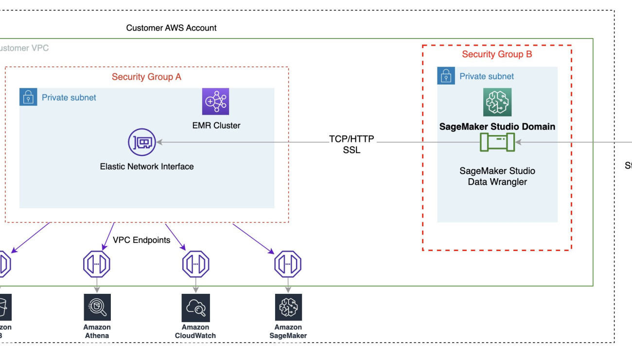
The following diagram represents the different components used in this solution.
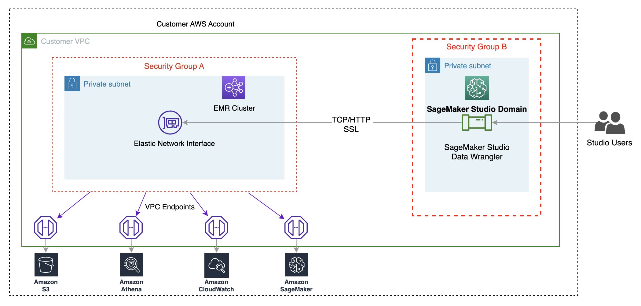
We demonstrate two authentication options that can be used to establish a connection to the EMR cluster. For each option, we deploy a unique stack of AWS CloudFormation templates.
The CloudFormation template performs the following actions when each option is selected:
- Creates a Studio Domain in VPC-only mode, along with a user profile named
studio-user. - Creates building blocks, including the VPC, endpoints, subnets, security groups, EMR cluster, and other required resources to successfully run the examples.
- For the EMR cluster, connects the AWS Glue Data Catalog as metastore for EMR Hive and Presto, creates a Hive table in EMR, and fills it with data from a US airport dataset.
- For the LDAP CloudFormation template, creates an Amazon Elastic Compute Cloud (Amazon EC2) instance to host the LDAP server to authenticate the Hive and Presto LDAP user.
Option 1: Lightweight Access Directory Protocol
For the LDAP authentication CloudFormation template, we provision an Amazon EC2 instance with an LDAP server and configure the EMR cluster to use this server for authentication. This is TLS enabled.
Option 2: No-Auth
In the No-Auth authentication CloudFormation template, we use a standard EMR cluster with no authentication enabled.
Deploy the resources with AWS CloudFormation
Complete the following steps to deploy the environment:
- Sign in to the AWS Management Console as an AWS Identity and Access Management (IAM) user, preferably an admin user.
- Choose Launch Stack to launch the CloudFormation template for the appropriate authentication scenario. Make sure the Region used to deploy the CloudFormation stack has no existing Studio Domain. If you already have a Studio Domain in a Region, you may choose a different Region.
LDAP 
No Auth 
- Choose Next.
- For Stack name, enter a name for the stack (for example,
dw-emr-hive-blog). - Leave the other values as default.
- To continue, choose Next from the stack details page and stack options.
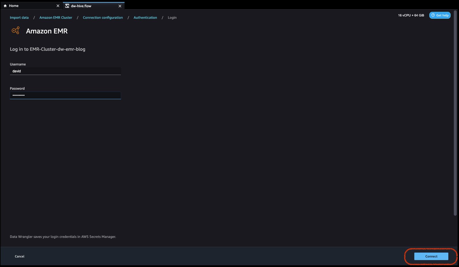
The LDAP stack uses the following credentials.- username:
david - password:
welcome123
- username:
- On the review page, select the check box to confirm that AWS CloudFormation might create resources.
- Choose Create stack. Wait until the status of the stack changes from
CREATE_IN_PROGRESStoCREATE_COMPLETE. The process usually takes 10–15 minutes.

Set up the Amazon EMR as a data source in Data Wrangler
In this section, we cover connecting to the existing Amazon EMR cluster created through the CloudFormation template as a data source in Data Wrangler.
Create a new data flow
To create your data flow, complete the following steps:
- On the SageMaker console, click Domains, then click on StudioDomain created by running above CloudFormation template.
- Select studio-user user profile and launch Studio.

- Choose Open studio.
- In the Studio Home console, choose Import & prepare data visually. Alternatively, on the File dropdown, choose New, then choose Data Wrangler Flow.
- Creating a new flow can take a few minutes. After the flow has been created, you see the Import data page.

- Add Amazon EMR as a data source in Data Wrangler. On the Add data source menu, choose Amazon EMR.

You can browse all the EMR clusters that your Studio execution role has permissions to see. You have two options to connect to a cluster; one is through interactive UI, and the other is to first create a secret using AWS Secrets Manager with JDBC URL, including EMR cluster information, and then provide the stored AWS secret ARN in the UI to connect to Hive. In this blog, we follow the first option.
- Select one of the following clusters that you want to use. Click on Next, and select endpoints.

- Select Hive, connect to Amazon EMR, create a name to identify your connection, and click Next.

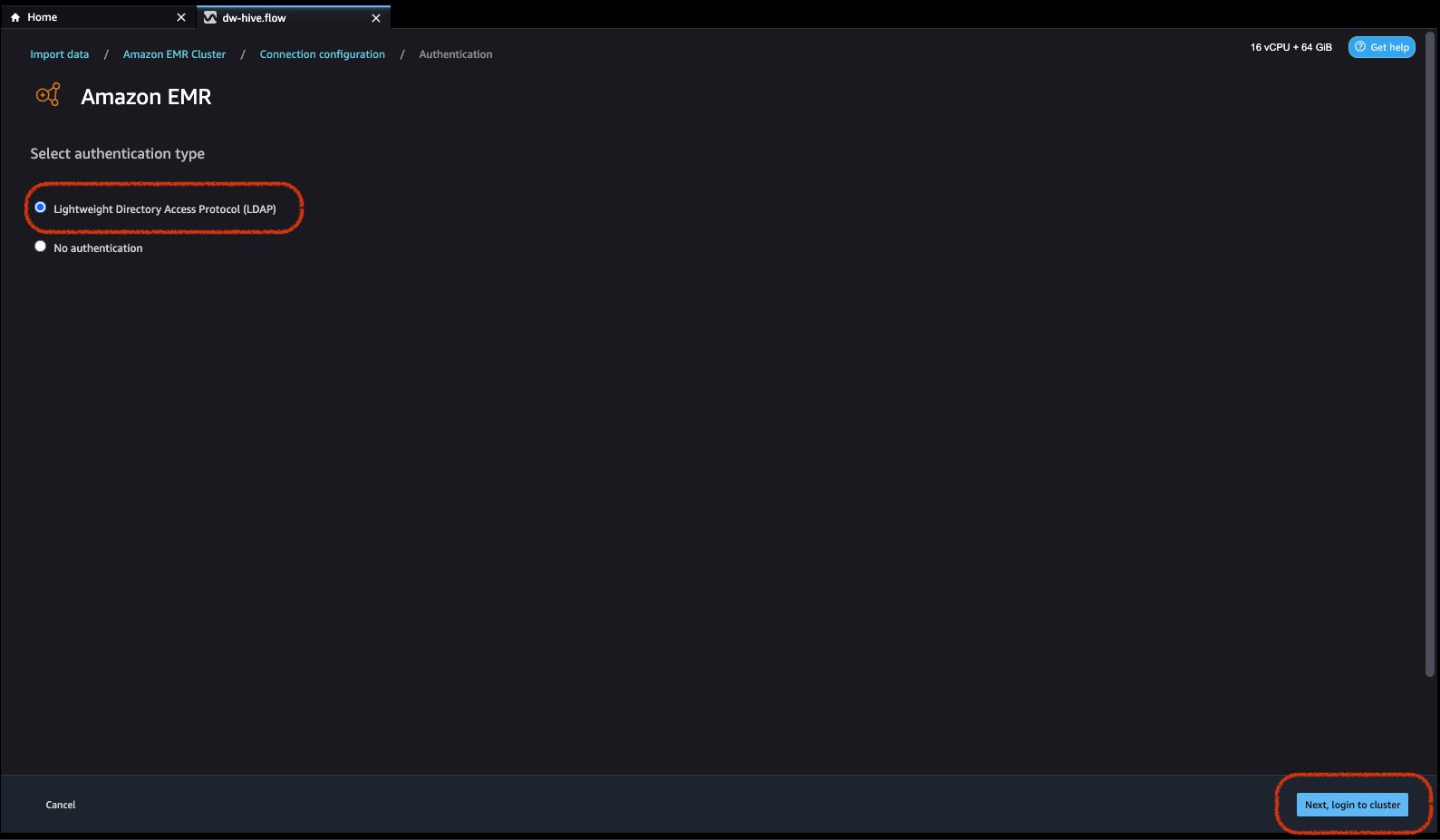
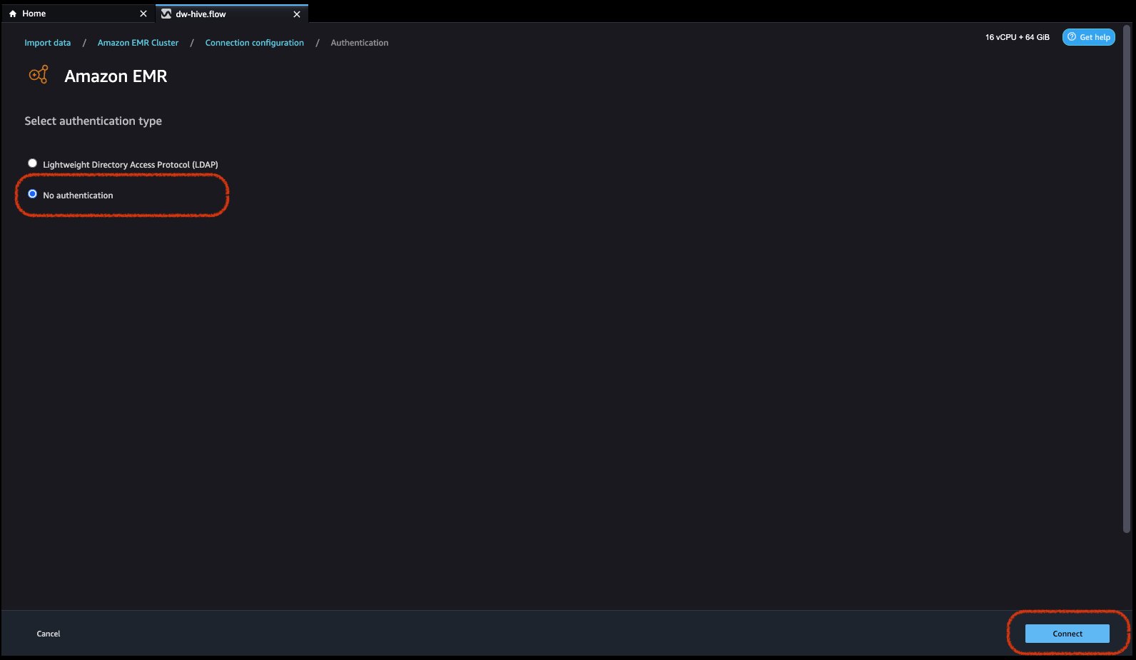
- Select authentication type, either Lightweight Directory Access Protocol (LDAP) or No authentication.
For Lightweight Directory Access Protocol (LDAP), select the option and click Next, login to cluster, then provide username and password to be authenticated and click Connect.
For No Authentication, you will be connected to EMR Hive without providing user credentials within VPC. Enter Data Wrangler’s SQL explorer page for EMR.
- Once connected, you can interactively view a database tree and table preview or schema. You can also query, explore, and visualize data from EMR. For preview, you would see a limit of 100 records by default. Once you provide a SQL statement in the query editor box and click the Run button, the query will be executed on EMR’s Hive engine to preview the data.

The Cancel query button allows ongoing queries to be canceled if they are taking an unusually long time.
- The last step is to import. Once you are ready with the queried data, you have options to update the sampling settings for the data selection according to the sampling type (FirstK, Random, or Stratified) and sampling size for importing data into Data Wrangler.
Click Import. The prepare page will be loaded, allowing you to add various transformations and essential analysis to the dataset.
- Navigate to Data flow from the top screen and add more steps to the flow as needed for transformations and analysis. You can run a data insight report to identify data quality issues and get recommendations to fix those issues. Let’s look at some example transforms.
- In the Data flow view, you should see that we are using EMR as a data source using the Hive connector.

- Let’s click on the + button to the right of Data types and select Add transform. When you do that, you will go back to the Data view.

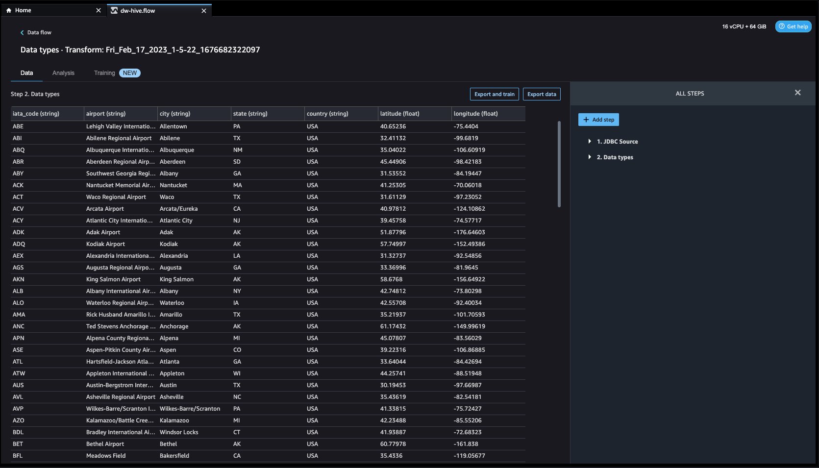
Let’s explore the data. We see that it has multiple features such as iata_code, airport, city, state, country, latitude, and longitude. We can see that the entire dataset is based in one country, which is the US, and there are missing values in latitude and longitude. Missing data can cause bias in the estimation of parameters, and it can reduce the representativeness of the samples, so we need to perform some imputation and handle missing values in our dataset.

- Let’s click on the Add Step button on the navigation bar to the right. Select Handle missing. The configurations can be seen in the following screenshots.
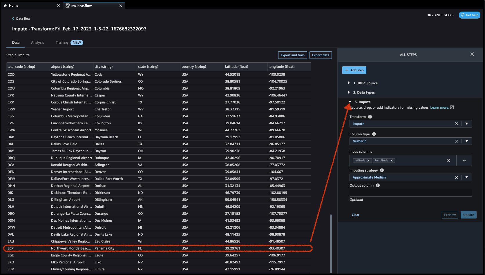
Under Transform, select Impute. Select the Column type as Numeric and Input column names latitude and longitude. We will be imputing the missing values using an approximate median value.
First click on Preview to view the missing value and then click on update to add the transform.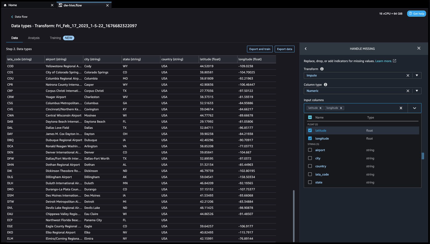
- Let us now look at another example transform. When building an ML model, columns are removed if they are redundant or don’t help your model. The most common way to remove a column is to drop it. In our dataset, the feature country can be dropped since the dataset is specifically for US airport data. To manage columns, click on the Add step button on the navigation bar to the right and select Manage columns. The configurations can be seen in the following screenshots. Under Transform, select Drop column, and under Columns to drop, select country.


- Click on Preview and then Update to drop the column.

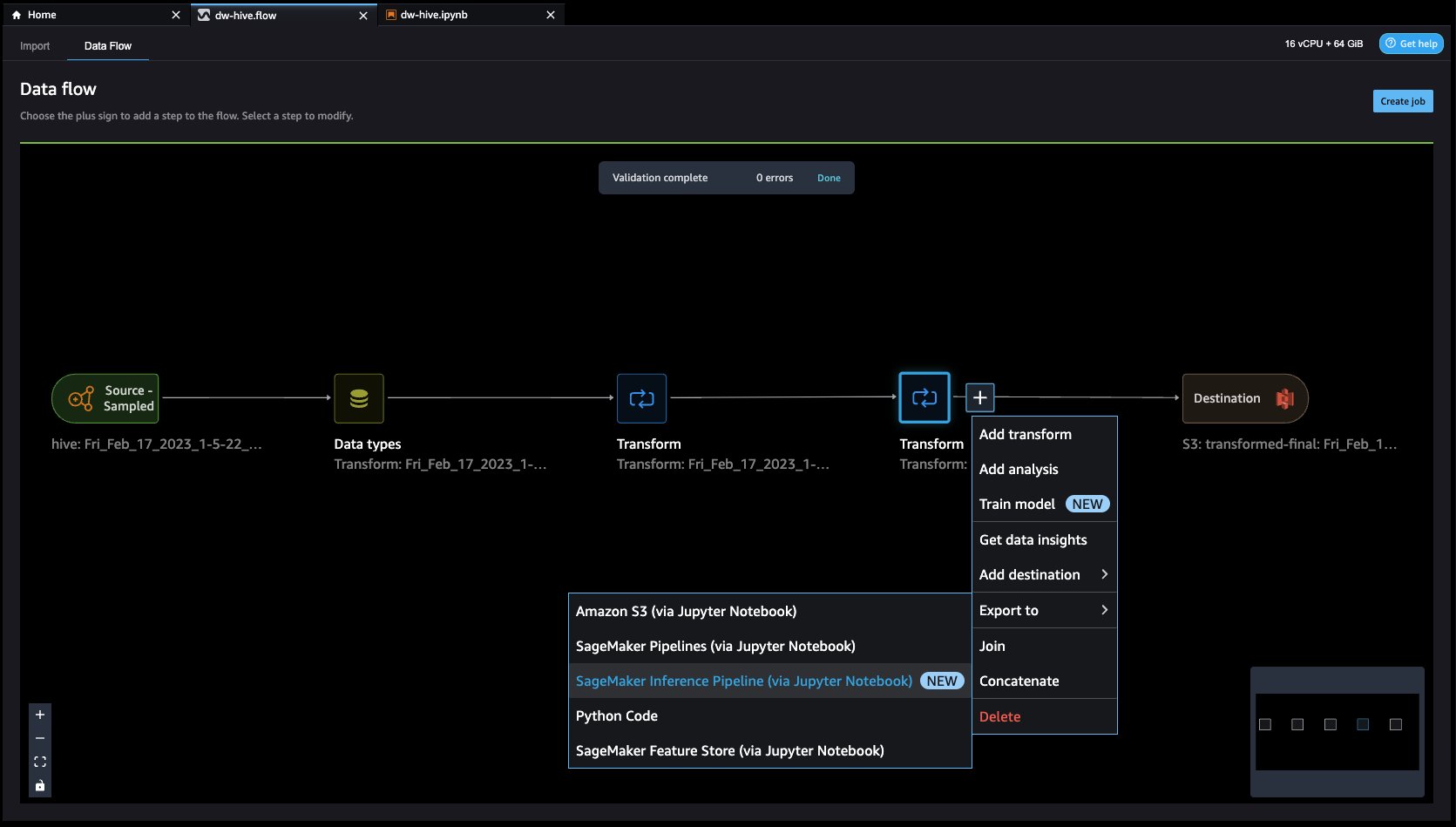
- Feature Store is a repository to store, share, and manage features for ML models. Let’s click on the + button to the right of Drop column. Select Export to and choose SageMaker Feature Store (via Jupyter notebook).

- By selecting SageMaker Feature Store as the destination, you can save the features into an existing feature group or create a new one.


We have now created features with Data Wrangler and easily stored those features in Feature Store. We showed an example workflow for feature engineering in the Data Wrangler UI. Then we saved those features into Feature Store directly from Data Wrangler by creating a new feature group. Finally, we ran a processing job to ingest those features into Feature Store. Data Wrangler and Feature Store together helped us build automatic and repeatable processes to streamline our data preparation tasks with minimum coding required. Data Wrangler also provides us flexibility to automate the same data preparation flow using scheduled jobs. We can also automatically train and deploy models using SageMaker Autopilot from Data Wrangler’s visual interface, or create training or feature engineering pipeline with SageMaker Pipelines (via Jupyter Notebook) and deploy to the inference endpoint with SageMaker inference pipeline (via Jupyter Notebook).
Clean up
If your work with Data Wrangler is complete, the following steps will help you delete the resources created to avoid incurring additional fees.
- Shut down SageMaker Studio.
From within SageMaker Studio, close all the tabs, then select File then Shut Down. Once prompted select Shutdown All.


Shutdown might take a few minutes based on the instance type. Make sure all the apps associated with the user profile got deleted. If they were not deleted, manually delete the app associated under user profile.

- Empty any S3 buckets that were created from CloudFormation launch.
Open the Amazon S3 page by searching for S3 in the AWS console search. Empty any S3 buckets that were created when provisioning clusters. The bucket would be of format dw-emr-hive-blog-.

- Delete the SageMaker Studio EFS.
Open the EFS page by searching for EFS in the AWS console search.
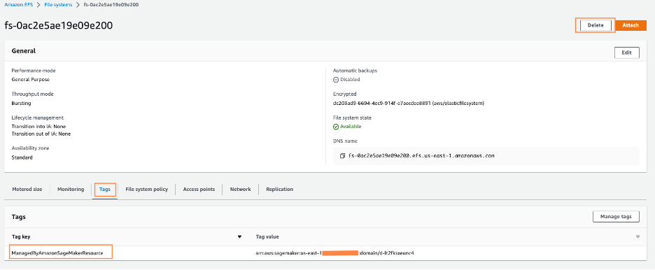
Locate the filesystem that was created by SageMaker. You can confirm this by clicking on the File system ID and confirming the tag ManagedByAmazonSageMakerResource on the Tags tab.
- Delete the CloudFormation stacks. Open CloudFormation by searching for and opening the CloudFormation service from the AWS console.
Select the template starting with dw- as shown in the following screen and delete the stack as shown by clicking on the Delete button.

This is expected and we will come back to this and clean it up in the subsequent steps.
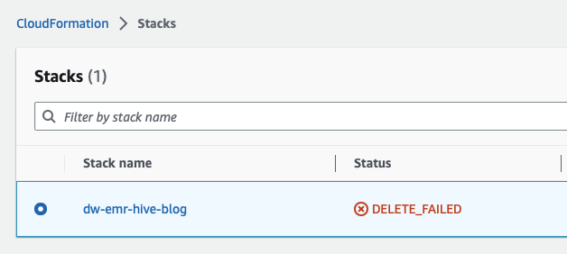
- Delete the VPC after the CloudFormation stack fails to complete. First open VPC from the AWS console.
- Next, identify the VPC that was created by the SageMaker Studio CloudFormation, titled
dw-emr-, and then follow the prompts to delete the VPC.
- Delete the CloudFormation stack.
Return to CloudFormation and retry the stack deletion for dw-emr-hive-blog.
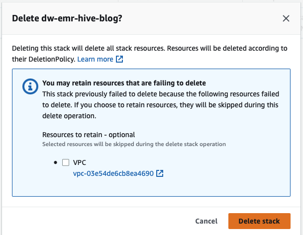
Complete! All the resources provisioned by the CloudFormation template described in this blog post will now be removed from your account.
Conclusion
In this post, we went over how to set up Amazon EMR as a data source in Data Wrangler, how to transform and analyze a dataset, and how to export the results to a data flow for use in a Jupyter notebook. After visualizing our dataset using Data Wrangler’s built-in analytical features, we further enhanced our data flow. The fact that we created a data preparation pipeline without writing a single line of code is significant.
To get started with Data Wrangler, see Prepare ML Data with Amazon SageMaker Data Wrangler and see the latest information on the Data Wrangler product page and AWS technical documents.
About the Authors
 Ajjay Govindaram is a Senior Solutions Architect at AWS. He works with strategic customers who are using AI/ML to solve complex business problems. His experience lies in providing technical direction as well as design assistance for modest to large-scale AI/ML application deployments. His knowledge ranges from application architecture to big data, analytics, and machine learning. He enjoys listening to music while resting, experiencing the outdoors, and spending time with his loved ones.
 Isha Dua is a Senior Solutions Architect based in the San Francisco Bay Area. She helps AWS enterprise customers grow by understanding their goals and challenges, and guides them on how they can architect their applications in a cloud-native manner while ensuring resilience and scalability. She’s passionate about machine learning technologies and environmental sustainability.
 Varun Mehta is a Solutions Architect at AWS. He is passionate about helping customers build Enterprise-Scale Well-Architected solutions on the AWS Cloud. He works with strategic customers who are using AI/ML to solve complex business problems.
Using Amazon SageMaker with Point Clouds: Part 1- Ground Truth for 3D labeling
In this two-part series, we demonstrate how to label and train models for 3D object detection tasks. In part 1, we discuss the dataset we’re using, as well as any preprocessing steps, to understand and label data. In part 2, we walk through how to train a model on your dataset and deploy it to production.
LiDAR (light detection and ranging) is a method for determining ranges by targeting an object or surface with a laser and measuring the time for the reflected light to return to the receiver. Autonomous vehicle companies typically use LiDAR sensors to generate a 3D understanding of the environment around their vehicles.
As LiDAR sensors become more accessible and cost-effective, customers are increasingly using point cloud data in new spaces like robotics, signal mapping, and augmented reality. Some new mobile devices even include LiDAR sensors. The growing availability of LiDAR sensors has increased interest in point cloud data for machine learning (ML) tasks, like 3D object detection and tracking, 3D segmentation, 3D object synthesis and reconstruction, and using 3D data to validate 2D depth estimation.
In this series, we show you how to train an object detection model that runs on point cloud data to predict the location of vehicles in a 3D scene. This post, we focus specifically on labeling LiDAR data. Standard LiDAR sensor output is a sequence of 3D point cloud frames, with a typical capture rate of 10 frames per second. To label this sensor output you need a labeling tool that can handle 3D data. Amazon SageMaker Ground Truth makes it easy to label objects in a single 3D frame or across a sequence of 3D point cloud frames for building ML training datasets. Ground Truth also supports sensor fusion of camera and LiDAR data with up to eight video camera inputs.
Data is essential to any ML project. 3D data in particular can be difficult to source, visualize, and label. We use the A2D2 dataset in this post and walk you through the steps to visualize and label it.
A2D2 contains 40,000 frames with semantic segmentation and point cloud labels, including 12,499 frames with 3D bounding box labels. Since we are focusing on object detection, we’re interested in the 12,499 frames with 3D bounding box labels. These annotations include 14 classes relevant to driving like car, pedestrian, truck, bus, etc.
The following table shows the complete class list:
| Index | Class list |
| 1 | animal |
| 2 | bicycle |
| 3 | bus |
| 4 | car |
| 5 | caravan transporter |
| 6 | cyclist |
| 7 | emergency vehicle |
| 8 | motor biker |
| 9 | motorcycle |
| 10 | pedestrian |
| 11 | trailer |
| 12 | truck |
| 13 | utility vehicle |
| 14 | van/SUV |
We will train our detector to specifically detect cars since that’s the most common class in our dataset (32616 of the 42816 total objects in the dataset are labeled as cars).
Solution overview
In this series, we cover how to visualize and label your data with Amazon SageMaker Ground Truth and demonstrate how to use this data in an Amazon SageMaker training job to create an object detection model, deployed to an Amazon SageMaker Endpoint. In particular, we’ll use an Amazon SageMaker notebook to operate the solution and launch any labeling or training jobs.
The following diagram depicts the overall flow of sensor data from labeling to training to deployment:

You’ll learn how to train and deploy a real-time 3D object detection model with Amazon SageMaker Ground Truth with the following steps:
- Download and visualize a point cloud dataset
- Prep data to be labeled with the Amazon SageMaker Ground Truth point cloud tool
- Launch a distributed Amazon SageMaker Ground Truth training job with MMDetection3D
- Evaluate your training job results and profiling your resource utilization with Amazon SageMaker Debugger
- Deploy an asynchronous SageMaker endpoint
- Call the endpoint and visualizing 3D object predictions
AWS services used to Implement this solution
- Amazon SageMaker Ground Truth
- Amazon SageMaker Training
- Amazon SageMaker Inference
- Amazon SageMaker Notebooks
- Amazon FSx for Lustre
- Amazon Simple Storage Service (Amazon S3)
Prerequisites
- An AWS account.
- Familiarity with Amazon SageMaker Ground Truth and AWS CloudFormation
- An Amazon SageMaker workforce. For this demonstration, we use a private workforce. You can create a workforce through the SageMaker console.
The following diagram demonstrates how to create a private workforce. For written, step-by-step instructions, see Create an Amazon Cognito Workforce Using the Labeling Workforces Page.
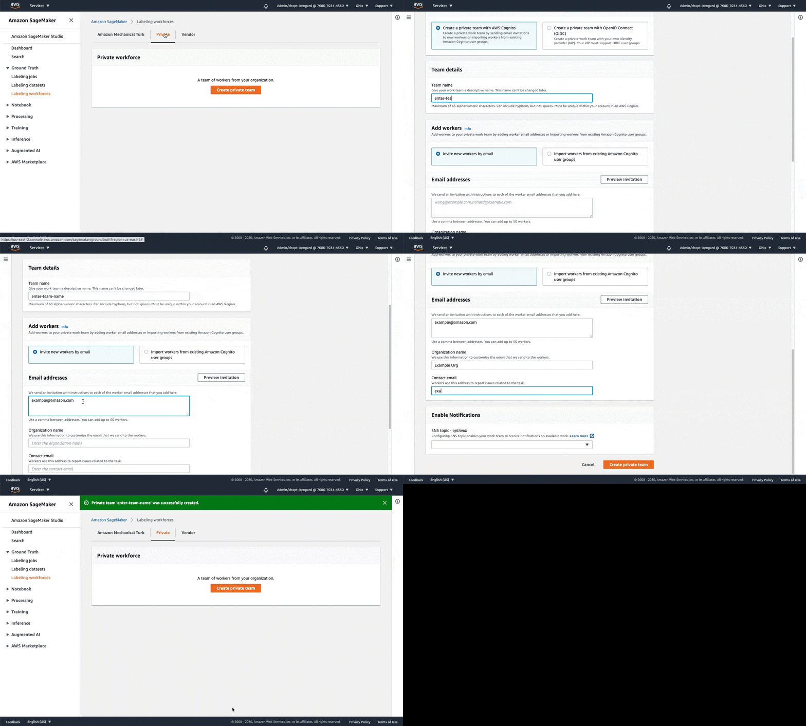
Launching the AWS CloudFormation stack
Now that you’ve seen the structure of the solution, you deploy it into your account so you can run an example workflow. All the deployment steps related to the labeling pipeline are managed by AWS CloudFormation. This means AWS Cloudformation creates your notebook instance as well as any roles or Amazon S3 Buckets to support running the solution.
You can launch the stack in AWS Region us-east-1 on the AWS CloudFormation console using the Launch Stack
button. To launch the stack in a different Region, use the instructions found in the README of the GitHub repository.
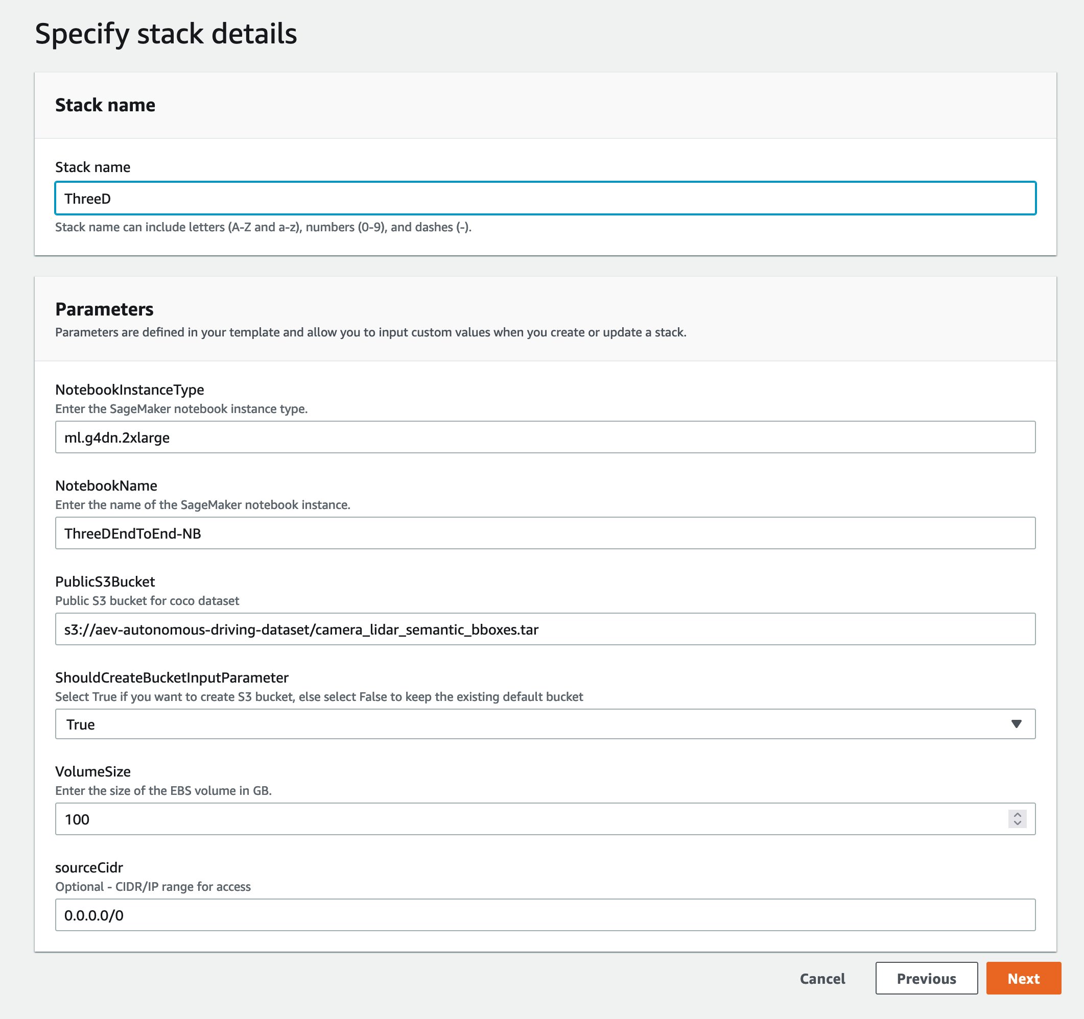
This takes approximately 20 minutes to create all the resources. You can monitor the progress from the AWS CloudFormation user interface (UI).
Once your CloudFormation template is done running go back to the AWS Console.
Opening the Notebook
Amazon SageMaker Notebook Instances are ML compute instances that run on the Jupyter Notebook App. Amazon SageMaker manages the creation of instances and related resources. Use Jupyter notebooks in your notebook instance to prepare and process data, write code to train models, deploy models to Amazon SageMaker hosting, and test or validate your models.
Follow the next steps to access the Amazon SageMaker Notebook environment:
- Under services search for Amazon SageMaker.

- Under Notebook, select Notebook instances.

- A Notebook instance should be provisioned. Select Open JupyterLab, which is located on the right side of the pre-provisioned Notebook instance under Actions.

- You’ll see an icon like this as the page loads:

- You’ll be redirected to a new browser tab that looks like the following diagram:

- Once you are in the Amazon SageMaker Notebook Instance Launcher UI. From the left sidebar, select the Git icon as shown in the following diagram.

- Select Clone a Repository option.

- Enter GitHub URL(https://github.com/aws-samples/end-2-end-3d-ml) in the pop‑up window and choose clone.

- Select File Browser to see the GitHub folder.

- Open the notebook titled
1_visualization.ipynb.
Operating the Notebook
Overview
The first few cells of the notebook in the section titled Downloaded Files walks through how to download the dataset and inspect the files within it. After the cells are executed, it takes a few minutes for the data to finish downloading.
Once downloaded, you can review the file structure of A2D2, which is a list of scenes or drives. A scene is a short recording of sensor data from our vehicle. A2D2 provides 18 of these scenes for us to train on, which are all identified by unique dates. Each scene contains 2D camera data, 2D labels, 3D cuboid annotations, and 3D point clouds.
You can view the file structure for the A2D2 dataset with the following:
A2D2 sensor setup
The next section walks through reading some of this point cloud data to make sure we’re interpreting it correctly and can visualize it in the notebook before trying to convert it into a format ready for data labeling.
For any kind of autonomous driving setup where we have 2D and 3D sensor data, capturing sensor calibration data is essential. In addition to the raw data, we also downloaded cams_lidar.json. This file contains the translation and orientation of each sensor relative to the vehicle’s coordinate frame, this can also be referred to as the sensor’s pose, or location in space. This is important for converting points from a sensor’s coordinate frame to the vehicle’s coordinate frame. In other words, it’s important for visualizing the 2D and 3D sensors as the vehicle drives. The vehicle’s coordinate frame is defined as a static point in the center of the vehicle, with the x-axis in the direction of the forward movement of the vehicle, the y-axis denoting left and right with left being positive, and the z-axis pointing through the roof of the vehicle. A point (X,Y,Z) of (5,2,1) means this point is 5 meters ahead of our vehicle, 2 meters to the left, and 1 meter above our vehicle. Having these calibrations also allows us to project 3D points onto our 2D image, which is especially helpful for point cloud labeling tasks.
To see the sensor setup on the vehicle, check the following diagram.
The point cloud data we are training on is specifically aligned with the front facing camera or cam front-center: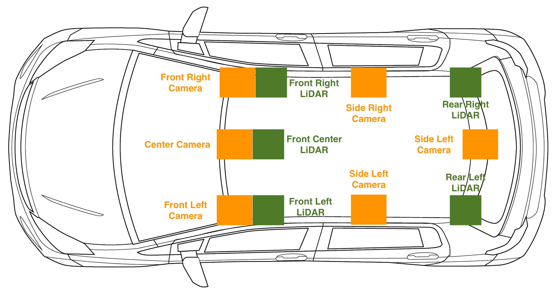
This matches our visualization of camera sensors in 3D:
This portion of the notebook walks through validating that the A2D2 dataset matches our expectations about sensor positions, and that we’re able to align data from the point cloud sensors into the camera frame. Feel free to run all cells through the one titled Projection from 3D to 2D to see your point cloud data overlay on the following camera image.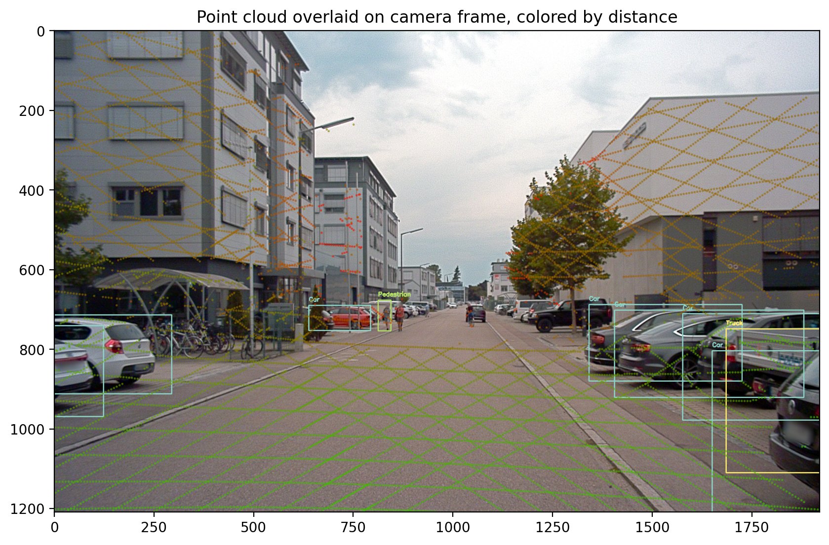
Conversion to Amazon SageMaker Ground Truth
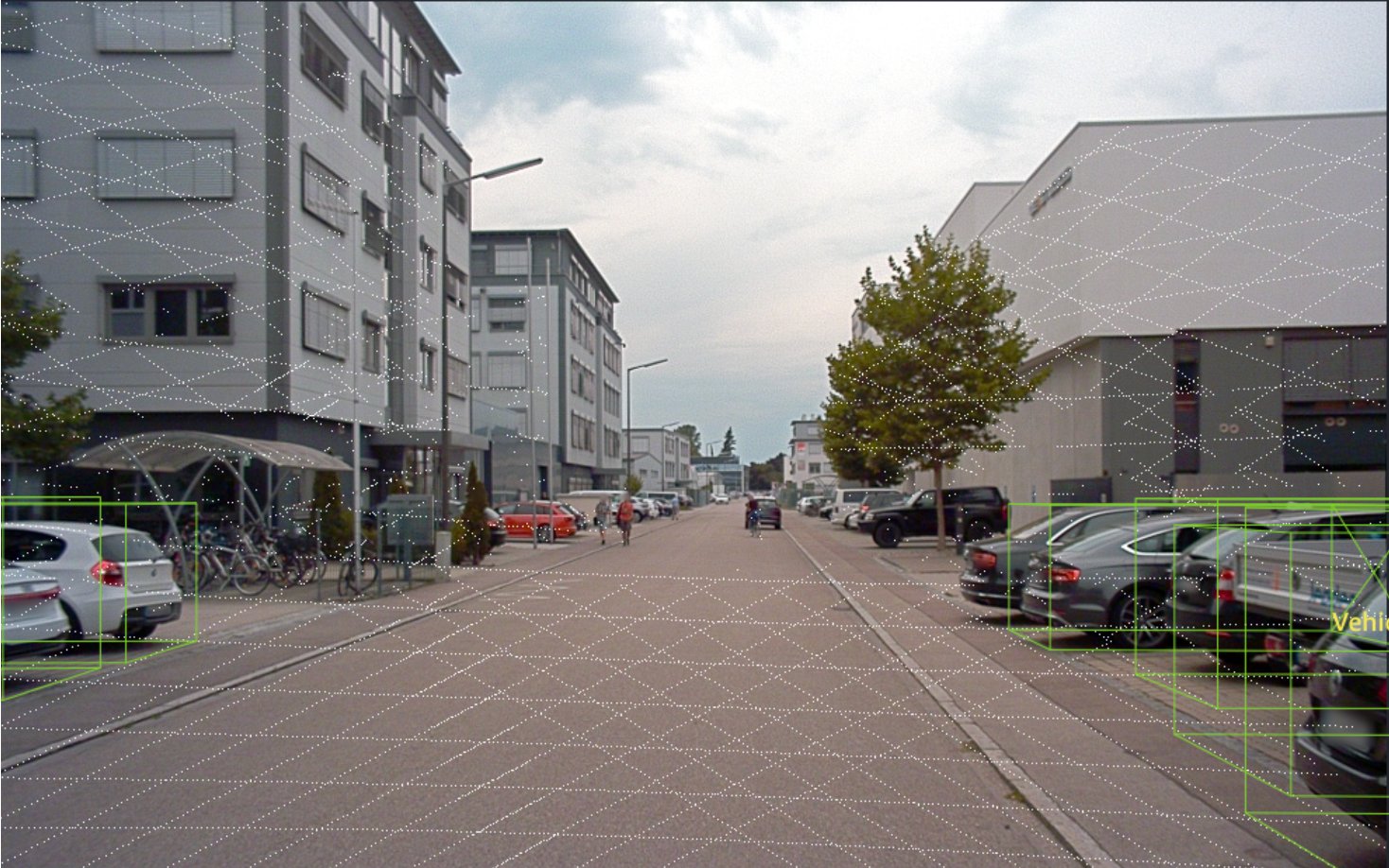
After visualizing our data in our notebook, we can confidently convert our point clouds into Amazon SageMaker Ground Truth’s 3D format to verify and adjust our labels. This section walks through converting from A2D2’s data format into an Amazon SageMaker Ground Truth sequence file, with the input format used by the object tracking modality.
The sequence file format includes the point cloud formats, the images associated with each point cloud, and all sensor position and orientation data required to align images with point clouds. These conversions are done using the sensor information read from the previous section. The following example is a sequence file format from Amazon SageMaker Ground Truth, which describes a sequence with only a single timestep.
The point cloud for this timestep is located at s3://sagemaker-us-east-1-322552456788/a2d2_smgt/20180807_145028_out/20180807145028_lidar_frontcenter_000000091.txt and has a format of <x coordinate> <y coordinate> <z coordinate>.
Associated with the point cloud, is a single camera image located at s3://sagemaker-us-east-1-322552456788/a2d2_smgt/20180807_145028_out/undistort_20180807145028_camera_frontcenter_000000091.png. Notice that we take the sequence file that defines all camera parameters to allow projection from the point cloud to the camera and back.
Conversion to this input format requires us to write a conversion from A2D2’s data format to data formats supported by Amazon SageMaker Ground Truth. This is the same process anyone must undergo when bringing their own data for labeling. We’ll walk through how this conversion works, step-by-step. If following along in the notebook, look at the function named a2d2_scene_to_smgt_sequence_and_seq_label.
Point cloud conversion
The first step is to convert the data from a compressed Numpy-formatted file (NPZ), which was generated with the numpy.savez method, to an accepted raw 3D format for Amazon SageMaker Ground Truth. Specifically, we generate a file with one row per point. Each 3D point is defined by three floating point X, Y, and Z coordinates. When we specify our format in the sequence file, we use the string text/xyz to represent this format. Amazon SageMaker Ground Truth also supports adding intensity values or Red Green Blue (RGB) points.
A2D2’s NPZ files contain multiple Numpy arrays, each with its own name. To perform a conversion, we load the NPZ file using Numpy’s load method, access the array called points (i.e., an Nx3 array, where N is the number of points in the point cloud), and save as text to a new file using Numpy’s savetxt method.
Image preprocessing
Next, we prepare our image files. A2D2 provides PNG images, and Amazon SageMaker Ground Truth supports PNG images; however, these images are distorted. Distortion often occurs because the image-taking lens is not aligned parallel to the imaging plane, which makes some areas in the image look closer than expected. This distortion describes the difference between a physical camera and an idealized pinhole camera model. If distortion isn’t taken into account, then Amazon SageMaker Ground Truth won’t be able to render our 3D points on top of the camera views, which makes it more challenging to perform labeling. For a tutorial on camera calibration, look at this documentation from OpenCV.
While Amazon SageMaker Ground Truth supports distortion coefficients in its input file, you can also perform preprocessing before the labeling job. Since A2D2 provides helper code to perform undistortion, we apply it to the image, and leave the fields related to distortion out of our sequence file. Note that the distortion related fields include k1, k2, k3, k4, p1, p2, and skew.
Camera position, orientation, and projection conversion
Beyond the raw data files required for labeling, the sequence file also requires camera position and orientation information to perform the projection of 3D points into the 2D camera views. We need to know where the camera is looking in 3D space to figure out how 3D cuboid labels and 3D points should be rendered on top of our images.
Because we’ve loaded our sensor positions into a common transform manager in the A2D2 sensor setup section, we can easily query the transform manager for the information we want. In our case, we treat the vehicle position as (0, 0, 0) in each frame because we don’t have position information of the sensor provided by A2D2’s object detection dataset. So relative to our vehicle, the camera’s orientation and position is described by the following code:
Now that position and orientation are converted, we also need to supply values for fx, fy, cx, and cy, all parameters for each camera in the sequence file format.
These parameters refer to values in the camera matrix. While the position and orientation describe which way a camera is facing, the camera matrix describes the field of the view of the camera and exactly how a 3D point relative to the camera gets converted to a 2D pixel location in an image.
A2D2 provides a camera matrix. A reference camera matrix is shown in the following code, along with how our notebook indexes this matrix to get the appropriate fields.
With all of the fields parsed from A2D2’s format, we can save the sequence file and use it in an Amazon SageMaker Ground Truth input manifest file to start a labeling job. This labeling job allows us to create 3D bounding box labels to use downstream for 3D model training.
Run all cells until the end of the notebook, and ensure you replace the workteam ARN with the Amazon SageMaker Ground Truth workteam ARN you created a prerequisite. After about 10 minutes of labeling job creation time, you should be able to login to the worker portal and use the labeling user interface to visualize your scene.
Clean up
Delete the AWS CloudFormation stack you deployed using the Launch Stack button named ThreeD in the AWS CloudFormation console to remove all resources used in this post, including any running instances.
Estimated costs
The approximate cost is $5 for 2 hours.
Conclusion
In this post, we demonstrated how to take 3D data and convert it into a form ready for labeling in Amazon SageMaker Ground Truth. With these steps, you can label your own 3D data for training object detection models. In the next post in this series, we’ll show you how to take A2D2 and train an object detector model on the labels already in the dataset.
Happy Building!
About the Authors
 Isaac Privitera is a Senior Data Scientist at the Amazon Machine Learning Solutions Lab, where he develops bespoke machine learning and deep learning solutions to address customers’ business problems. He works primarily in the computer vision space, focusing on enabling AWS customers with distributed training and active learning.
 Vidya Sagar Ravipati is Manager at the Amazon Machine Learning Solutions Lab, where he leverages his vast experience in large-scale distributed systems and his passion for machine learning to help AWS customers across different industry verticals accelerate their AI and cloud adoption. Previously, he was a Machine Learning Engineer in Connectivity Services at Amazon who helped to build personalization and predictive maintenance platforms.
 Jeremy Feltracco is a Software Development Engineer with th Amazon Machine Learning Solutions Lab at Amazon Web Services. He uses his background in computer vision, robotics, and machine learning to help AWS customers accelerate their AI adoption.
Real-time fraud detection using AWS serverless and machine learning services
Online fraud has a widespread impact on businesses and requires an effective end-to-end strategy to detect and prevent new account fraud and account takeovers, and stop suspicious payment transactions. Detecting fraud closer to the time of fraud occurrence is key to the success of a fraud detection and prevention system. The system should be able to detect fraud as effectively as possible also alert the end-user as quickly as possible. The user can then choose to take action to prevent further abuse.
In this post, we show a serverless approach to detect online transaction fraud in near-real time. We show how you can apply this approach to various data streaming and event-driven architectures, depending on the desired outcome and actions to take to prevent fraud (such as alert the user about the fraud or flag the transaction for additional review).
This post implements three architectures:
- Streaming data inspection and fraud detection/prevention – Using Amazon Kinesis Data Streams, AWS Lambda, AWS Step Functions, and Amazon Fraud Detector
- Streaming data enrichment for fraud detection/prevention – Using Amazon Kinesis Data Firehose, AWS Lambda, and Amazon Fraud Detector
- Event data inspection and fraud detection/prevention – Using Amazon EventBridge, AWS Step Functions, and Amazon Fraud Detector
To detect fraudulent transactions, we use Amazon Fraud Detector, a fully managed service enabling you to identify potentially fraudulent activities and catch more online fraud faster. To build an Amazon Fraud Detector model based on past data, refer to Detect online transaction fraud with new Amazon Fraud Detector features. You can also use Amazon SageMaker to train a proprietary fraud detection model. For more information, refer to Train fraudulent payment detection with Amazon SageMaker.
Streaming data inspection and fraud detection/prevention
This architecture uses Lambda and Step Functions to enable real-time Kinesis data stream data inspection and fraud detection and prevention using Amazon Fraud Detector. The same architecture applies if you use Amazon Managed Streaming for Apache Kafka (Amazon MSK) as a data streaming service. This pattern can be useful for real-time fraud detection, notification, and potential prevention. Example use cases for this could be payment processing or high-volume account creation. The following diagram illustrates the solution architecture.

The flow of the process in this implementation is as follows:
- We ingest the financial transactions into the Kinesis data stream. The source of the data could be a system that generates these transactions—for example, ecommerce or banking.
- The Lambda function receives the transactions in batches.
- The Lambda function starts the Step Functions workflow for the batch.
- For each transaction, the workflow performs the following actions:
- Persist the transaction in an Amazon DynamoDB table.
- Call the Amazon Fraud Detector API using the GetEventPrediction action. The API returns one of the following results: approve, block, or investigate.
- Update the transaction in the DynamoDB table with fraud prediction results.
- Based on the results, perform one of the following actions:
- Send a notification using Amazon Simple Notification Service (Amazon SNS) in case of a block or investigate response from Amazon Fraud Detector.
- Process the transaction further in case of an approve response.
This approach allows you to react to the potentially fraudulent transactions in real time as you store each transaction in a database and inspect it before processing further. In actual implementation, you may replace the notification step for additional review with an action that is specific to your business process—for example, inspect the transaction using some other fraud detection model, or conduct a manual review.
Streaming data enrichment for fraud detection/prevention
Sometimes, you may need to flag potentially fraudulent data but still process it; for example, when you’re storing the transactions for further analytics and collecting more data for constantly tuning the fraud detection model. An example use case is claims processing. During claims processing, you collect all the claims documents and then run them through a fraud detection system. A decision to process or reject a claim is then made—not necessarily in real time. In such cases, streaming data enrichment may fit your use case better.
This architecture uses Lambda to enable real-time Kinesis Data Firehose data enrichment using Amazon Fraud Detector and Kinesis Data Firehose data transformation.
This approach doesn’t implement fraud prevention steps. We deliver enriched data to an Amazon Simple Storage Service (Amazon S3) bucket. Downstream services that consume the data can use the fraud detection results in their business logics and act accordingly. The following diagram illustrates this architecture.

The flow of the process in this implementation is as follows:
- We ingest the financial transactions into Kinesis Data Firehose. The source of the data could be a system that generates these transactions, such as ecommerce or banking.
- A Lambda function receives the transactions in batches and enriches them. For each transaction in the batch, the function performs the following actions:
- Call the Amazon Fraud Detector API using the GetEventPrediction action. The API returns one of three results: approve, block or investigate.
- Update transaction data by adding fraud detection results as metadata.
- Return the batch of the updated transactions to the Kinesis Data Firehose delivery stream.
- Kinesis Data Firehose delivers data to the destination (in our case, the S3 bucket).
As a result, we have data in the S3 bucket that includes not only original data but also the Amazon Fraud Detector response as metadata for each of the transactions. You can use this metadata in your data analytics solutions, machine learning model training tasks, or visualizations and dashboards that consume transaction data.
Event data inspection and fraud detection/prevention
Not all data comes into your system as a stream. However, in cases of event-driven architectures, you still can follow a similar approach.
This architecture uses Step Functions to enable real-time EventBridge event inspection and fraud detection/prevention using Amazon Fraud Detector. It doesn’t stop processing of the potentially fraudulent transaction, rather it flags the transaction for an additional review. We publish enriched transactions to an event bus that differs from the one that raw event data is being published to. This way, consumers of the data can be sure that all events include fraud detection results as metadata. The consumers can then inspect the metadata and apply their own rules based on the metadata. For example, in an event-driven ecommerce application, a consumer can choose to not process the order if this transaction is predicted to be fraudulent. This architecture pattern can also be useful for detecting and preventing fraud in new account creation or during account profile changes (like changing your address, phone number, or credit card on file in your account profile). The following diagram illustrates the solution architecture.

The flow of the process in this implementation is as follows:
- We publish the financial transactions to an EventBridge event bus. The source of the data could be a system that generates these transactions—for example, ecommerce or banking.
- The EventBridge rule starts the Step Functions workflow.
- The Step Functions workflow receives the transaction and processes it with the following steps:
- Call the Amazon Fraud Detector API using the
GetEventPredictionaction. The API returns one of three results: approve, block, or investigate. - Update transaction data by adding fraud detection results.
- If the transaction fraud prediction result is block or investigate, send a notification using Amazon SNS for further investigation.
- Publish the updated transaction to the EventBridge bus for enriched data.
- Call the Amazon Fraud Detector API using the
As in the Kinesis Data Firehose data enrichment method, this architecture doesn’t prevent fraudulent data from reaching the next step. It adds fraud detection metadata to the original event and sends notifications about potentially fraudulent transactions. It may be that consumers of the enriched data don’t include business logics that use fraud detection metadata in their decisions. In that case, you can change the Step Functions workflow so it doesn’t put such transactions to the destination bus and routes them to a separate event bus to be consumed by a separate suspicious transactions processing application.
Implementation
For each of the architectures described in this post, you can find AWS Serverless Application Model (AWS SAM) templates, deployment, and testing instructions in the sample repository.
Conclusion
This post walked through different methods to implement a real-time fraud detection and prevention solution using Amazon Machine Learning services and serverless architectures. These solutions allow you to detect fraud closer to the time of fraud occurrence and act on it as quickly as possible. The flexibility of the implementation using Step Functions allows you to react in a way that is most appropriate for the situation and also adjust prevention steps with minimal code changes.
For more serverless learning resources, visit Serverless Land.
About the Authors
 Veda Raman is a Senior Specialist Solutions Architect for machine learning based in Maryland. Veda works with customers to help them architect efficient, secure and scalable machine learning applications. Veda is interested in helping customers leverage serverless technologies for Machine learning.
 Giedrius Praspaliauskas is a Senior Specialist Solutions Architect for serverless based in California. Giedrius works with customers to help them leverage serverless services to build scalable, fault-tolerant, high-performing, cost-effective applications.
How Vodafone Uses TensorFlow Data Validation in their Data Contracts to Elevate Data Governance at Scale

Posted by Amandeep Singh (Vodafone), Max Vökler (Google Cloud)
Vodafone leverages Google Cloud to deploy AI/ML use cases at scale
As one of the largest telecommunications companies worldwide, Vodafone is working with Google Cloud to advance their entire data landscape, including their data lake, data warehouse (DWH), and in particular AI/ML strategies. While Vodafone has used AI/ML for some time in production, the growing number of use cases has posed challenges for industrialization and scalability. For Vodafone, it is key to rapidly build and deploy ML use cases at scale in a highly regulated industry. While Vodafone’s AI Booster Platform – built on top of Google Cloud’s Vertex AI – has provided a huge step to achieve that, this blog post will dive into how TensorFlow Data Validation (TFDV) helps advance data governance at scale.
High-quality Data is a Prerequisite for ML Use Cases, yet not Easily Achieved
Excelling in data governance is a key enabler to utilize the AI Booster Platform at scale. As Vodafone works in distributed teams and has shared responsibilities when developing use cases, it is important to avoid disruptions across the involved parties:
- Machine Learning Engineer at Vodafone Group level (works on global initiatives and provides best practices on productionizing ML at scale)
- Data Scientist in local market (works on a concrete implementation for their specific country, needs to ensure proper data quality and feature engineering)
- Data Owner in local market (needs to ensure data schemas do not change)
An issue that often arises is that table schemas are modified, or feature names and data types change. This could be due to a variety of reasons. For example, the data engineering process, which is owned by IT teams, is revised.
Data Contracts Define the Expected Form and Shape of Data
Data Contracts in machine learning are a set of rules that define the structure, data types, and constraints of the data that your models are trained on. The contracts provide a way to specify the expected schema and statistics of your data. The following can be included as part of your Data Contract:
- Feature names
- Data types
- Expected distribution of values in each column.
It can also include constraints on the data, such as:
- Minimum and maximum values for numerical columns
- Allowed values for categorical columns.
Before a model is productionized, the Contract is agreed upon by the stakeholders working on the pipeline, such as the ML Engineers, Data Scientists and Data Owners. Once the Data Contract is agreed upon, it cannot change. If a pipeline breaks due to a change, the error can be traced back to the responsible party. If the Contract needs amending, it needs to go to a review between the stakeholders, and once agreed upon, the changes can be implemented into the pipeline. This helps ensure the quality of data going into our model in production.
Vodafone Benefits from TFDV Data Contracts as a Way to Streamline Data Governance
As part of Vodafone’s efforts to streamline data governance, we made use of Data Contracts. A Data Contract ensures all teams work in unison, helping to maintain quality throughout the data lifecycle. These contacts are a powerful tool for managing and validating data used for machine learning. They provide a way to ensure that data is of high quality, free of errors and has the expected distribution. This blog post covers the basics of Data Contracts, discusses how they can be used to validate and understand your data better, and shows you how to use them in combination with TFDV to improve the accuracy and performance of your ML models. Whether you’re a data scientist, an ML engineer, or a developer working with machine learning, understanding Data Contracts is essential for building high-quality, accurate models.
How Vodafone Uses Data Contracts
Utilizing such a Data Contract, both in training and prediction pipelines, we can detect and diagnose issues such as outliers, inconsistencies, and errors in the data before they can cause problems with the models. Another great use of using Data Contracts is that it helps us detect data drift. Data drift is the most common reason for performance degradation in ML Models. Data drift is when the input data to your model changes to what it was trained on, leading to errors and inaccuracies in your predictions. Using Data Contracts can help you identify this issue.
Data Contracts are just one example of the many KPIs we have within Vodafone regarding AI Governance and Scalability. Since the development and release of AI Booster, more and more markets are using the platform to productionize their use case, and as part of this, we have the resources to scale components vertically. Examples of this, apart from Data Contracts, can be specialized logging, agreed-upon ways of calculating Model Metrics and Model Testing strategies, such as Champion/Challenger and A/B Testing.
How TensorFlow Data Validation (TFDV) Brings Data Contracts to Life
TFDV is a library provided by the TensorFlow team, for analyzing and validating machine learning data. It provides a way to check that the data conforms to a Data Contract. TFDV also provides visualization options to help developers understand the data, such as histograms and summary statistics. It allows the user to define data constraints and detect errors, anomalies, and drift between datasets. This can help to detect and diagnose issues such as outliers, inconsistencies, and errors in your data before they can cause problems with your models.
When you use TFDV to validate your data, it will check that the data has the expected schema. If there are any discrepancies, such as a missing column or a column with the wrong datatype, TFDV will raise an error and provide detailed information about the problem.
At Vodafone, before a pipeline is put into production, a schema is agreed upon for the input data. The agreement is between the Product Manager/Use Case Owner, Data Owner, Data Scientist and ML Engineer. The first thing we do in our pipeline, as seen in Figure 1, is to generate statistics about our data.
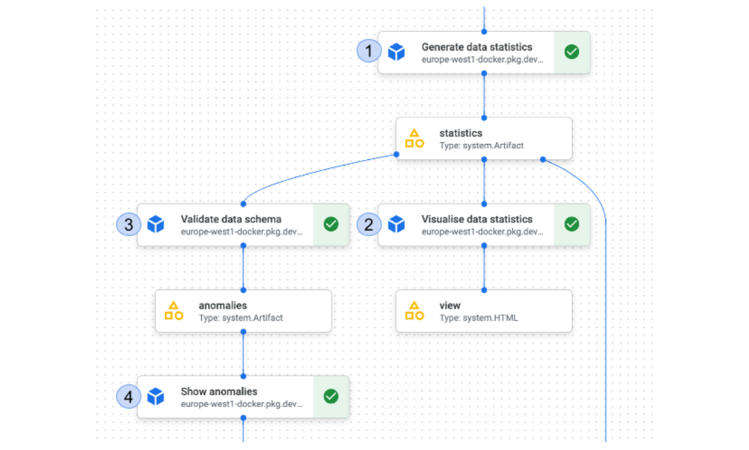 |
| Figure 1: Components of a Data Contract in a typical Vodafone training pipeline |
The code below uses TFDV to generate statistics for the training dataset and visualizes them (step 2), making it easy to understand the distribution of the data and how it’s been transformed. The output of this step is an HTML file, displaying general statistics about our input dataset. You can also choose a range of different functionalities on the HTML webpage to play around with the statistics and get a deeper understanding of the data.
# generate training statisticsgen_statistics = generate_statistics( dataset=train_dataset.output, file_pattern=file_pattern, ).set_display_name("Generate data statistics") # visualise statisticsvisualised_statistics = visualise_statistics( statistics=gen_statistics.output, statistics_name="Training Statistics").set_display_name("Visualise data statistics") |
Step 3 is concerned with validating the schema. Within our predefined schema, we also define some thresholds for certain data fields. We can specify domain constraints on our Data Contract, such as minimum and maximum values for numerical columns or allowed values for categorical columns. When you validate your data, TFDV will check that all the values in the dataset are within the specified domain. If any values are out of range, TFDV will provide a warning and give you the option to either discard or correct the data. There is also the possibility to specify the expected distribution of values in each feature of the Data Contract. TFDV will compute the actual statistics of your data, as shown in Figure 2, and compare them to the expected distribution. If there are any significant discrepancies, TFDV will provide a warning and give you the option to investigate the data further.
Furthermore, this allows us to detect outliers and anomalies in the data (step 4) by comparing the actual statistics of your data to the expected statistics. It can flag any data points that deviate significantly from the expected distribution and provide visualizations to help you understand the nature of the anomaly.
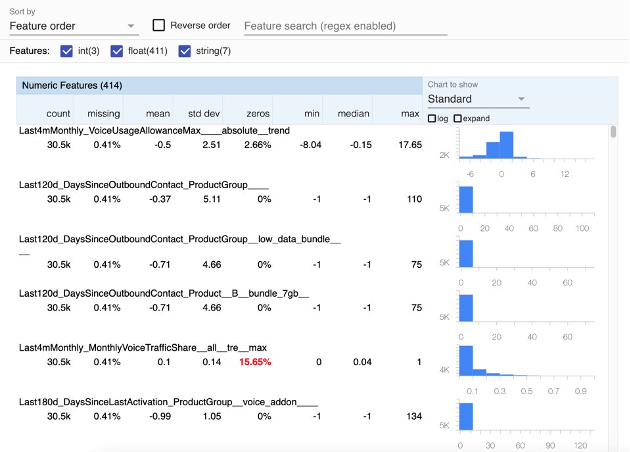 |
| Figure 2: Example visualization of the dataset statistics created by TFDV |
This code below is using the TFDV library to validate the data schema and detect any anomalies. The validate_schema function takes two arguments, statistics, and schema_path. Statistics argument is the output of a previous step which is generating statistics, and schema_path is the path to the schema file that was constructed in the first line. This function checks if the data conforms to the schema specified in the schema file.
# Construct schema_path from base GCS path + filenametfdv_schema_path = ( f"{pipeline_files_gcs_path}/{tfdv_schema_filename}") # validate data schemavalidated_schema = validate_schema( statistics=gen_statistics.output, schema_path=tfdv_schema_path ).set_display_name("Validate data schema") # show anomalies and fail if any anomalies were detectedanomalies = show_anomalies( anomalies=validated_schema.output, fail_on_anomalies=True).set_display_name("Show anomalies") |
The next block calls the show_anomalies function which takes two arguments, anomalies and fail_on_anomalies. The anomalies argument is the output of the previous validate_schema function, which includes the detected anomalies if any. The fail_on_anomalies argument is a flag that when set to true, will fail the pipeline if any anomalies are detected. This function will display the anomalies if any were detected, which looks something like this.
anomaly_info { key: "producer_used" value { description: "Examples contain values missing from the schema: Microsoft (<1%), Sony Ericsson (<1%), Xiaomi (<1%), Samsung (<1%), IPhone (<1%). " severity: ERROR short_description: "Unexpected string values" reason { type: ENUM_TYPE_UNEXPECTED_STRING_VALUES short_description: "Unexpected string values" description: "Examples contain values missing from the schema: Microsoft (<1%), Sony Ericsson (<1%), Xiaomi (<1%), Samsung (<1%), IPhone (<1%). " } path { step: "producer_used" } } } |
All the above components were developed internally using Custom KFP components and TFDV.
How Vodafone Industrialized the Approach on its AI Booster Platform
As part of the AI Booster platform, we have also provided templates for different Modeling Libraries such as XGBoost, TensorFlow, AutoML and BigQuery ML. These templates, which are based on Kubeflow Pipelines (KFP) pipelines, offer a wide range of customizable components that can be easily integrated into your machine learning workflow.
Our templates provide a starting point for our Data Scientists and ML Engineers, but they are fully customizable to fit their specific needs. However, we do enforce the inclusion of certain components in the pipeline when it is being productionized. As shown in Figure 1, we require that all production pipelines include Data Contract components. These components are not specific to a particular model and are intended to be used whenever data is being ingested for training or prediction.
Automating this step helps with our data validation process, making it more efficient and less prone to human error. It gives all stakeholders the confidence that whenever the model is in production, the data being used by the Model is always up to standard and not full of surprises. In addition, it helps with reproducibility of use cases in different markets, using local data. But most importantly it helps with Compliance and Privacy. It ensures us that our data is being used in compliance with company policies and regulations, and provides a framework for tracking and monitoring the usage of the data to make sure that it is being used appropriately.
Data Contracts with TFDV Helped Vodafone Industrialize their ML Workflow
Data Contracts play a critical role in ensuring the quality and integrity of the data used in machine learning models. Data Contracts provide:
- a set of rules and guidelines for how data should be collected, stored, and used, and help to ensure that the data is of high quality and free of errors
- a framework for identifying and resolving issues with the data, such as outliers, inconsistencies, and errors, before they can cause problems with the models
- a way to ensure compliance with company policies and regulations
- a way to trace back the origin and history of the data, which can be useful for auditing and troubleshooting purposes
They also help to ensure that the data is being used consistently and in a reproducible way, which can help to improve the accuracy and performance of the models and reduce the risk of errors and inaccuracies in the predictions. Data contracts used in conjunction with tools like TFDV help automate the data validation process, making it more efficient and less prone to human error. Applying this concept in AI Booster helped us at Vodafone to make a key step forward in industrializing our AI/ML use cases.
Find Out More
For more information about TFDV, see the user guide and tutorials on tensorflow.org. Special thanks to Amandeep Singh of Vodafone and Max Vökler of Google Cloud for their work to create this design and for writing this post.

