Architect personalized generative AI SaaS applications on Amazon SageMaker

Architect personalized generative AI SaaS applications on Amazon SageMaker

The AI landscape is being reshaped by the rise of generative models capable of synthesizing high-quality data, such as text, images, music, and videos. The course toward democratization of AI helped to further popularize generative AI following the open-source releases for such foundation model families as BERT, T5, GPT, CLIP and, most recently, Stable Diffusion. Hundreds of software as a service (SaaS) applications are being developed around these pre-trained models, which are either directly served to end-customers, or fine-tuned first on a per-customer basis to generate personal and unique content (such as avatars, stylized photo edits, video game assets, domain-specific text, and more). With the pace of technological innovation and proliferation of novel use cases for generative AI, upcoming AI-native SaaS providers and startups in the B2C segment need to prepare for scale from day one, and aim to shorten their time-to-market by reducing operational overhead as much as possible.

In this post, we review the technical requirements and application design considerations for fine-tuning and serving hyper-personalized AI models at scale on AWS. We propose an architecture based on the fully managed Amazon SageMaker training and serving features that enables SaaS providers to develop their applications faster, provide quality of service, and increase cost-effectiveness.

Solution scope and requirements

Let’s first define the scope for personalized generative AI SaaS applications:

Next, let’s review the technical requirements and workflow for an application that supports fine-tuning and serving of potentially thousands of personalized models. The workflow generally consists of two parts:

  • Generate a personalized model via lightweight fine-tuning of the base pre-trained model
  • Host the personalized model for on-demand inference requests when the user returns

One of the considerations for the first part of the workflow is that we should be prepared for unpredictable and spiky user traffic. The peaks in usage could arise, for example, due to new foundation model releases or fresh SaaS feature rollouts. This will impose large intermittent GPU capacity needs, as well as a need for asynchronous fine-tuning job launches to absorb the traffic spike.

With respect to model hosting, as the market floods with AI-based SaaS applications, speed of service becomes a distinguishing factor. A snappy, smooth user experience could be impaired by infrastructure cold starts or high inference latency. Although inference latency requirements will depend on the use case and user expectations, in general this consideration leads to a preference for real-time model hosting on GPUs (as opposed to slower CPU-only hosting options). However, real-time GPU model hosting can quickly lead to high operational costs. Therefore, it’s vital for us to define a hosting strategy that will prevent costs from growing linearly with the number of deployed models (active users).

Solution architecture

Before we describe the proposed architecture, let’s discuss why SageMaker is a great fit for our application requirements by looking at some of its features.

First, SageMaker Training and Hosting APIs provide the productivity benefit of fully managed training jobs and model deployments, so that fast-moving teams can focus more time on product features and differentiation. Moreover, the launch-and-forget paradigm of SageMaker Training jobs perfectly suits the transient nature of the concurrent model fine-tuning jobs in the user onboarding phase. We discuss more considerations on concurrency in the next section.

Second, SageMaker supports unique GPU-enabled hosting options for deploying deep learning models at scale. For example, NVIDIA Triton Inference Server, a high-performance open-source inference software, was natively integrated into the SageMaker ecosystem in 2022. This was followed by the launch of GPU support for SageMaker multi-model endpoints, which provides a scalable, low-latency, and cost-effective way to deploy thousands of deep learning models behind a single endpoint.

Finally, when we get down to the infrastructure level, these features are backed by best-in-class compute options. For example, the G5 instance type, which is equipped with NVIDIA A10g GPUs (unique to AWS), offers a strong price-performance ratio, both for model training and hosting. It yields a lowest cost per FP32 FLOP (an important measure of how much compute power you get per dollar) across the GPU-instance palette on AWS, and greatly improves on the previous lowest cost GPU instance type (G4dn). For more information, refer to Achieve four times higher ML inference throughput at three times lower cost per inference with Amazon EC2 G5 instances for NLP and CV PyTorch models.

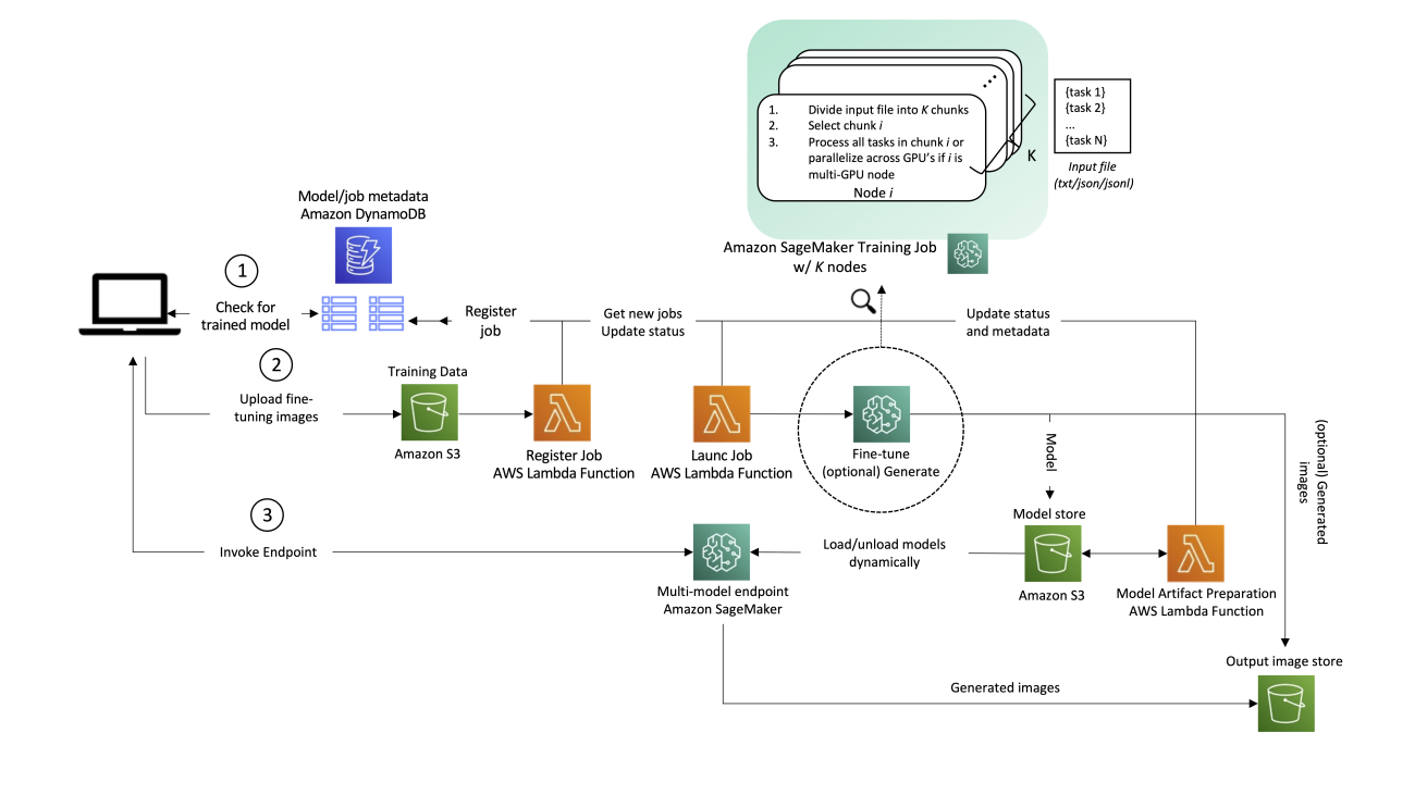
Although the following architecture generally applies to various generative AI use cases, let’s use text-to-image generation as an example. In this scenario, an image generation app will create one or multiple custom, fine-tuned models for each of its users, and those models will be available for real-time image generation on demand by the end-user. The solution workflow can then be divided into two major phases, as is evident from the architecture. The first phase (A) corresponds to the user onboarding process—this is when a model is fine-tuned for the new user. In the second phase (B), the fine-tuned model is used for on-demand inference.

Proposed architecture

Let’s go through the steps in the architecture in more detail, as numbered in the diagram.

1. Model status check

When a user interacts with the service, we first check if it’s a returning user that has already been onboarded to the service and has personalized models ready for serving. A single user might have more than one personalized model. The mapping between user and corresponding models is saved in Amazon DynamoDB, which serves as a fully managed, serverless, non-relational metadata store, which is easy to query, inexpensive, and scalable. At a minimum, we recommend having two tables:

  • One to store the mapping between users and models. This includes the user ID and model artifact Amazon Simple Storage Service (Amazon S3) URI.
  • Another to serve as a queue, storing the model creation requests and their completion status. This includes the user ID, model training job ID, and status, along with hyperparameters and metadata associated with training.

2. User onboarding and model fine-tuning.

If no model has been fine-tuned for the user before, the application uploads fine-tuning images to Amazon S3, triggering an AWS Lambda function to register a new job to a DynamoDB table.

Another Lambda function queries the table for a new job and launches it with SageMaker Training. It can be triggered for each record using Amazon DynamoDB Streams, or on a schedule using Amazon EventBridge (a pattern that is tried and tested by AWS customers, including internally at Amazon). Optionally, images or prompts can be passed for inference, and processed directly in the SageMaker Training job right after the model is trained. This can help shorten the time to deliver the first images back to the application. As images are generated, you can exploit the checkpoint sync mechanism in SageMaker to upload intermediate results to Amazon S3. Regarding job launch concurrency, the SageMaker CreateTrainingJob API supports a request rate of one per second, with larger burst rates available during high traffic periods. If you sustainably need to launch more than one fine-tuning task per second (TPS), you have the following controls and options:

  • Use SageMaker Managed Warm Pools, which let you retain and reuse provisioned infrastructure after the completion of a training job to reduce cold start latency for repetitive workloads.
  • Implement retries in your launch job Lambda function (shown in the architecture diagram).
  • Ultimately, if the fine-tuning request rate will consistently be above 1 TPS, you can launch N fine-tunings in parallel with a single SageMaker Training job by requesting a job with num_instances=K, and spreading the work over the different instances. An example of how you can achieve this is to pass a list of tasks to be run as an input file to the training job, and each instance processes a different task or chunk of this file, differentiated by the instance’s numerical identifier (found in resourceconfig.json). Keep in mind individual tasks shouldn’t differ greatly in training duration, so as to avoid the situation where a single task keeps the whole cluster up and running for longer than needed.

Finally, the fine-tuned model is saved, triggering a Lambda function that prepares the artifact for serving on a SageMaker multi-model endpoint. At this point, the user could be notified that training is complete and the model is ready for use. Refer to Managing backend requests and frontend notifications in serverless web apps for best practices on this.

3. On-demand serving of user requests

If a model has been previously fine-tuned for the user, the path is much simpler. The application invokes the multi-model endpoint, passing the payload and the user’s model ID. The selected model is dynamically loaded from Amazon S3 onto the endpoint instance’s disk and GPU memory (if it has not been recently used; for more information, refer to How multi-model endpoints work), and used for inference. The model output (personalized content) is finally returned to the application.

The request input and output should be saved to S3 for the user’s future reference. To avoid impacting request latency (the time measured from the moment a user makes a request until a response is returned), you can do this upload directly from the client application, or alternatively within your endpoint’s inference code.

This architecture provides the asynchrony and concurrency that were part of the solution requirements.

Conclusion

In this post, we walked through considerations to fine-tune and serve hyper-personalized AI models at scale, and proposed a flexible, cost-efficient solution on AWS using SageMaker.

We didn’t cover the use case of large model pre-training. For more information, refer to Distributed Training in Amazon SageMaker and Sharded Data Parallelism, as well as stories on how AWS customers have trained massive models on SageMaker, such as AI21 and Stability AI.


About the Authors

João Moura is an AI/ML Specialist Solutions Architect at AWS, based in Spain. He helps customers with deep learning model training and inference optimization, and more broadly building large-scale ML platforms on AWS. He is also an active proponent of ML-specialized hardware and low-code ML solutions.

Dr. Alexander Arzhanov is an AI/ML Specialist Solutions Architect based in Frankfurt, Germany. He helps AWS customers to design and deploy their ML solutions across EMEA region. Prior to joining AWS, Alexander was researching origins of heavy elements in our universe and grew passionate about ML after using it in his large-scale scientific calculations.

Olivier Cruchant is a Machine Learning Specialist Solutions Architect at AWS, based in France. Olivier helps AWS customers – from small startups to large enterprises – develop and deploy production-grade machine learning applications. In his spare time, he enjoys reading research papers and exploring the wilderness with friends and family.

Heiko Hotz is a Senior Solutions Architect for AI & Machine Learning with a special focus on natural language processing (NLP), large language models (LLMs), and generative AI. Prior to this role, he was the Head of Data Science for Amazon’s EU Customer Service. Heiko helps our customers be successful in their AI/ML journey on AWS and has worked with organizations in many industries, including insurance, financial services, media and entertainment, healthcare, utilities, and manufacturing. In his spare time, Heiko travels as much as possible.

Read More

Use a data-centric approach to minimize the amount of data required to train Amazon SageMaker models

Use a data-centric approach to minimize the amount of data required to train Amazon SageMaker models

As machine learning (ML) models have improved, data scientists, ML engineers and researchers have shifted more of their attention to defining and bettering data quality. This has led to the emergence of a data-centric approach to ML and various techniques to improve model performance by focusing on data requirements. Applying these techniques allows ML practitioners to reduce the amount of data required to train an ML model.

As part of this approach, advanced data subset selection techniques have surfaced to speed up training by reducing input data quantity. This process is based on automatically selecting a given number of points that approximate the distribution of a larger dataset and using it for training. Applying this type of technique reduces the amount of time required to train an ML model.

In this post, we describe applying data-centric AI principles with Amazon SageMaker Ground Truth, how to implement data subset selection techniques using the CORDS repository on Amazon SageMaker to reduce the amount of data required to train an initial model, and how to run experiments using this approach with Amazon SageMaker Experiments.

A data-centric approach to machine learning

Before diving into more advanced data-centric techniques like data subset selection, you can improve your datasets in multiple ways by applying a set of underlying principles to your data labeling process. For this, Ground Truth supports various mechanisms to improve label consistency and data quality.

Label consistency is important for improving model performance. Without it, models can’t produce a decision boundary that separates every point belonging to differing classes. One way to ensure consistency is by using annotation consolidation in Ground Truth, which allows you to serve a given example to multiple labelers and use the aggregated label provided as the ground truth for that example. Divergence in the label is measured by the confidence score generated by Ground Truth. When there is divergence in labels, you should look to see if there is ambiguity in the labeling instructions provided to your labelers that can be removed. This approach mitigates the effects of bias of individual labelers, which is central to making labels more consistent.

Another way to improve model performance by focusing on data involves developing methods to analyze errors in labels as they come up to identify the most important subset of data to improve upon. you can do this for your training dataset with a combination of manual efforts involving diving into labeled examples and using the Amazon CloudWatch logs and metrics generated by Ground Truth labeling jobs. It’s also important to look at errors the model makes at inference time to drive the next iteration of labeling for our dataset. In addition to these mechanisms, Amazon SageMaker Clarify allows data scientists and ML engineers to run algorithms like KernelSHAP to allow them to interpret predictions made by their model. As mentioned, a deeper explanation into the model’s predictions can be related back to the initial labeling process to improve it.

Lastly, you can consider tossing out noisy or overly redundant examples. Doing this allows you to reduce training time by removing examples that don’t contribute to improving model performance. However, identifying a useful subset of a given dataset manually is difficult and time consuming. Applying the data subset selection techniques described in this post allows you to automate this process along established frameworks.

Use case

As mentioned, data-centric AI focuses on improving model input rather than the architecture of the model itself. Once you have applied these principles during data labeling or feature engineering, you can continue to focus on model input by applying data subset selection at training time.

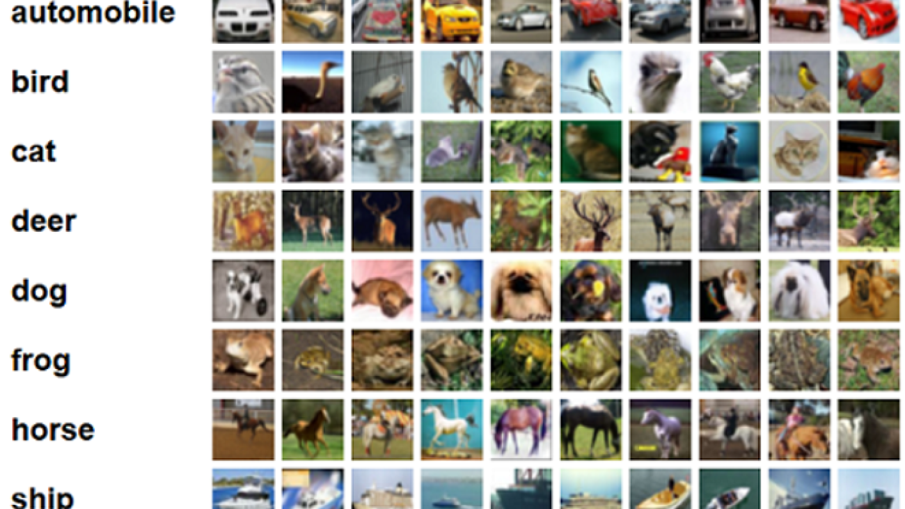
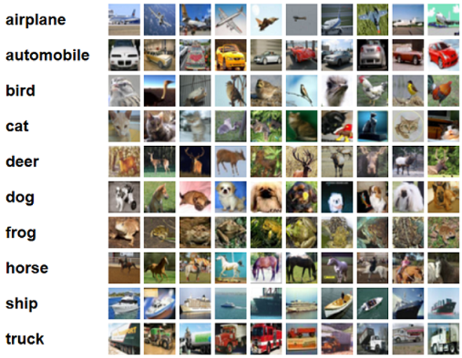
For this post, we apply Generalization based Data Subset Selection for Efficient and Robust Learning (GLISTER), which is one of many data subset selection techniques implemented in the CORDS repository, to the training algorithm of a ResNet-18 model to minimize the time it takes to train a model to classify CIFAR-10 images. The following are some sample images with their respective labels pulled from the CIFAR-10 dataset.

CIFAR Dataset

ResNet-18 is often used for classification tasks. It is an 18-layer deep convolutional neural network. The CIFAR-10 dataset is often used to evaluate the validity of various techniques and approaches in ML. It’s composed of 60,000 32×32 color images labeled across 10 classes.

In the following sections, we show how GLISTER can help you answer the following question to some degree:

What percentage of a given dataset can we use and still achieve good model performance during training?

Applying GLISTER to your training algorithm will introduce fraction as a hyperparameter in your training algorithm. This represents the percentage of the given dataset you wish to use. As with any hyperparameter, finding the value producing the best result for your model and data requires tuning. We don’t go in depth into hyperparameter tuning in this post. For more information, refer to Optimize hyperparameters with Amazon SageMaker Automatic Model Tuning.

We run several tests using SageMaker Experiments to measure the impact of the approach. Results will vary depending on the initial dataset, so it’s important to test the approach against our data at different subset sizes.

Although we discuss using GLISTER on images, you can also apply it to training algorithms working with structured or tabular data.

Data subset selection

The purpose of data subset selection is to accelerate the training process while minimizing the effects on accuracy and increasing model robustness. More specifically, GLISTER-ONLINE selects a subset as the model learns by attempting to maximize the log-likelihood of that training data subset on the validation set you specify. Optimizing data subset selection in this way mitigates against the noise and class imbalance that is often found in real-world datasets and allows the subset selection strategy to adapt as the model learns.

The initial GLISTER paper describes a speedup/accuracy trade-off at various data subset sizes as followed using a LeNet model:

Subset size Speedup Accuracy
10% 6x -3%
30% 2.5x -1.20%
50% 1.5x -0.20%

To train the model, we run a SageMaker training job using a custom training script. We have also already uploaded our image dataset to Amazon Simple Storage Service (Amazon S3). As with any SageMaker training job, we need to define an Estimator object. The PyTorch estimator from the sagemaker.pytorch package allows us to run our own training script in a managed PyTorch container. The inputs variable passed to the estimator’s .fit function contains a dictionary of the training and validation dataset’s S3 location.

The train.py script is run when a training job is launched. In this script, we import the ResNet-18 model from the CORDS library and pass it the number of classes in our dataset as follows:

from cords.utils.models import ResNet18

numclasses = 10
model = ResNet18(numclasses)

Then, we use the gen_dataset function from CORDS to create training, validation, and test datasets:

from cords.utils.data.datasets.SL import gen_dataset

train_set, validation_set, test_set, numclasses = gen_dataset(
datadir="/opt/ml/input/data/training",
dset_name="cifar10",
feature="dss",
type="image")

From each dataset, we create an equivalent PyTorch dataloader:

train_loader = torch.utils.data.DataLoader(train_set,
batch_size=batch_size,
shuffle=True)

validation_loader = torch.utils.data.DataLoader(validation_set,
batch_size=batch_size,
shuffle=False)

Lastly, we use these dataloaders to create a GLISTERDataLoader from the CORDS library. It uses an implementation of the GLISTER-ONLINE selection strategy, which applies subset selection as we update the model during training, as discussed earlier in this post.

To create the object, we pass the selection strategy specific arguments as a DotMap object along with the train_loader, validation_loader, and logger:

import logging
from cords.utils.data.dataloader.SL.adaptive import GLISTERDataLoader
from dotmap import DotMap

dss_args = # GLISTERDataLoader specific arguments
dss_args = DotMap(dss_args)
dataloader = GLISTERDataLoader(train_loader,
validation_loader,
dss_args,
logger,
batch_size=batch_size,
shuffle=True,
pin_memory=False)

The GLISTERDataLoader can now be applied as a regular dataloader to a training loop. It will select data subsets for the next training batch as the model learns based on that model’s loss. As demonstrated in the preceding table, adding a data subset selection strategy allows us to significantly reduce training time, even with the additional step of data subset selection, with little trade-off in accuracy.

Data scientists and ML engineers often need to evaluate the validity of an approach by comparing it with some baseline. We demonstrate how to do this in the next section.

Experiment tracking

You can use SageMaker Experiments to measure the validity of the data subset selection approach. For more information, see Next generation Amazon SageMaker Experiments – Organize, track, and compare your machine learning trainings at scale.

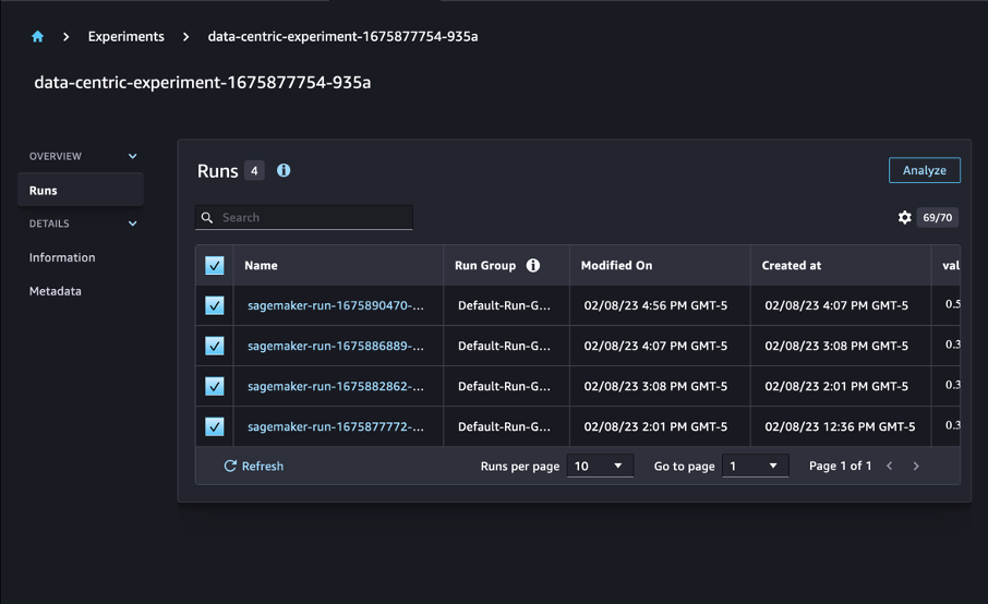
In our case, we perform four experiments: a baseline without applying data subset selection, and three others with differing fraction parameters, which represents the size of the subset relative to the overall dataset. Naturally, using a smaller fraction parameter should result in reduced training times, but lower model accuracy as well.

For this post, each training run is represented as a Run in SageMaker Experiments. The runs related to our experiment are all grouped under one Experiment object. Runs can be attached to a common experiment when creating the Estimator with the SDK. See the following code:

from sagemaker.utils import unique_name_from_base
from sagemaker.experiments.run import Run, load_run

experiment_name = unique_name_from_base("data-centric-experiment")
with Run(
experiment_name=experiment_name,
sagemaker_session=sess
) as run:
estimator = PyTorch('train.py',
source_dir="source",
role=role,
instance_type=instance_type,
instance_count=1,
framework_version=framework_version,
py_version='py3',
env={
'SAGEMAKER_REQUIREMENTS': 'requirements.txt',
})
estimator.fit(inputs)

As part of your custom training script, you can collect run metrics by using load_run:

from sagemaker.experiments.run import load_run
from sagemaker.session import Session

if __name__ == "__main__":
args = parse_args()
session = Session(boto3.session.Session(region_name=args.region))
with load_run(sagemaker_session=session) as run:
train(args, run)

Then, using the run object returned by the previous operation, u can collect data points per epoch by calling run.log_metric(name, value, step) and supplying the metric name, value, and current epoch number.

To measure the validity of our approach, we collect metrics corresponding to training loss, training accuracy, validation loss, validation accuracy, and time to complete an epoch. Then, after running the training jobs, we can review the results of our experiment in Amazon SageMaker Studio or through the SageMaker Experiments SDK.

To view validation accuracies within Studio, choose Analyze on the experiment Runs page.

Experiments List

Add a chart, set the chart properties, and choose Create. As shown in the following screenshot, you’ll see a plot of validation accuracies at each epoch for all runs.

Experiments Chart

The SDK also allows you to retrieve experiment-related information as a Pandas dataframe:

from sagemaker.analytics import ExperimentAnalytics

trial_component_analytics = ExperimentAnalytics(
sagemaker_session=sess.sagemaker_client,
experiment_name=experiment_name
)
analytic_table = trial_component_analytics.dataframe()

Optionally, the training jobs can be sorted. For instance, we could add "metrics.validation:accuracy.max" as the value of the sort_by parameter passed to ExperimentAnalytics to return the result ordered by validation accuracy.

As expected, our experiments show that applying GLISTER and data subset selection to the training algorithm reduces training time. When running our baseline training algorithm, the median time to complete a single epoch hovers around 27 seconds. By contrast, applying GLISTER to select a subset equivalent to 50%, 30%, and 10% of the overall dataset results in times to complete an epoch of about 13, 8.5, and 2.75 seconds, respectively, on ml.p3.2xlarge instances.

We also observe a comparatively minimal impact on validation accuracy, especially when using data subsets of 50%. After training for 100 epochs, the baseline produces a validation accuracy of 92.72%. In contrast, applying GLISTER to select a subset equivalent to 50%, 30%, and 10% of the overall dataset results in validation accuracies of 91.42%, 89.76%, and 82.82%, respectively.

Conclusion

SageMaker Ground Truth and SageMaker Experiments enable a data-centric approach to machine learning by allowing data scientists and ML engineers to produce more consistent datasets and track the impact of more advanced techniques as they implement them in the model building phase. Implementing a data-centric approach to ML allows you to reduce the amount of data required by your model and improve its robustness.

Give it a try, and let us know what you think in comments.


About the authors

Nicolas Bernier is a Solutions Architect, part of the Canadian Public Sector team at AWS. He is currently conducting a master’s degree with a research area in Deep Learning and holds five AWS certifications, including the ML Specialty Certification. Nicolas is passionate about helping customers deepen their knowledge of AWS by working with them to translate their business challenges into technical solutions.

Givanildo Alves is a Prototyping Architect with the Prototyping and Cloud Engineering team at Amazon Web Services, helping clients innovate and accelerate by showing the art of possible on AWS, having already implemented several prototypes around artificial intelligence. He has a long career in software engineering and previously worked as a Software Development Engineer at Amazon.com.br.


Read More

Race to the Cloud: EA’s ‘GRID Legends’ Now Streaming on GeForce NOW

Race to the Cloud: EA’s ‘GRID Legends’ Now Streaming on GeForce NOW

It’s a thrilling GFN Thursday with GRID Legends racing to the cloud this week. It leads a total of eight new games expanding the GeForce NOW library. New content for Rainbow Six Siege is also now streaming.

Plus, two new cities are now online with GeForce RTX 4080 performance for cloud gaming. Chicago and Montreal have completed upgrades to RTX 4080 SuperPODs, delivering next-generation cloud streaming to GeForce NOW Ultimate members.

Shifting Up

GRID Legends GeForce NOW
Beyond-fast gaming meets beyond-fast racing.

Jump into the spectacular action of GRID Legends, the racing game from EA with drama at every turn. Battle for glory with a variety of incredible cars on stellar tracks featuring iconic landmarks from the streets of London and Moscow.

Navigate the world of high-stakes racing as a rookie behind the wheel, with a documentary team capturing every sensational moment. Conquer hundreds of events and challenges, and create a dream racing team in the unique, cinematic story mode. Join up online with other legends and race against friends, or challenge them to a race designed in the Race Creator mode.

GeForce NOW members can experience it all with high dynamic range on PC, Mac and SHIELD TV for a smooth, ultra-crisp driving experience, even under intense racing conditions.

Upgrade Roll Call

GeForce NOW Ultimate SuperPOD Rollout
Order up! Servers are now live in Chicago and Montreal.

The RTX 4080 SuperPODs have been rolling out around the world for a couple months now, so it’s time to check in with a RTX 4080 roll call.

Chicago and Montreal bring the number of cities on the server update map to 10, joining Ashburn, Dallas, Los Angeles and San Jose in the U.S., and Amsterdam, Frankfurt, London and Paris in Europe. Now past it’s halfway point, the rollout is expected to be completed by mid-year.

Here’s a few reasons to upgrade:

  • NVIDIA DLSS 3 technology is enabled for AI-powered performance boosts on supported games like HITMAN World of Assassination and Marvel’s Midnight Suns. This means 4K streaming from the cloud results in the smoothest game play at up to 120 frames per second, even when settings are cranked to the max.
  • NVIDIA Reflex delivers ultra-low latency. Paired with DLSS 3, the technology enables Ultimate members to stream games like Rainbow Six Siege and Apex Legends at up to 240 fps on PCs and Macs, with as low as 35 milliseconds of total latency for a streaming experience that feels nearly indistinguishable from being on a local desktop.
  • Ultrawide resolutions are supported for the first time ever from the cloud, giving Ultimate members the most immersive game play in No Man’s Sky, Cyberpunk 2077 and Assassin’s Creed Valhalla.

Ultimate members in and around the 10 cities on the map are streaming with new performance today, and can take full advantage of these RTX technologies in the cloud. Level up to next-generation cloud streaming today for beyond-fast gaming.

Spring Forward With New Games

Rainbow Six Siege Season 1 Year 8 on GeForce NOW
“Brava will do what’s needed. Even when it requires sacrifice.”

Operation Commanding Force is the newest season of Year 8 for Tom Clancy’s Rainbow Six Siege, now available for members to stream. The update brings a new attacker named Brava, equipped with the Kludge Drone, a gadget that can disrupt enemy electronics devices and even take over some of them to turn the tides of battle.

That’s on top of the eight games joining the cloud this week:

  • Hotel Renovator (New release on Steam)
  • Clash: Artifacts of Chaos (New release on Steam, March 9)
  • Figment 2: Creed Valley (New release on Steam, March 9)
  • Monster Energy Supercross – The Official Videogame 6 (New release on Steam, March 9)
  • Big Ambitions (New release on Steam, March 10)
  • Call of the Sea (Free on Epic Games, March 9)
  • GRID Legends (Steam and EA)
  • Scars Above (Steam)

There’s a whole lot of games streaming from the cloud, and we want to know your top three. Let us know in the comments below or on Twitter and Facebook.

Read More

Use Snowflake as a data source to train ML models with Amazon SageMaker

Use Snowflake as a data source to train ML models with Amazon SageMaker

Amazon SageMaker is a fully managed machine learning (ML) service. With SageMaker, data scientists and developers can quickly and easily build and train ML models, and then directly deploy them into a production-ready hosted environment. Sagemaker provides an integrated Jupyter authoring notebook instance for easy access to your data sources for exploration and analysis, so you don’t have to manage servers. It also provides common ML algorithms that are optimized to run efficiently against extremely large data in a distributed environment.

SageMaker requires that the training data for an ML model be present either in Amazon Simple Storage Service (Amazon S3), Amazon Elastic File System (Amazon EFS) or Amazon FSx for Lustre (for more information, refer to Access Training Data). In order to train a model using data stored outside of the three supported storage services, the data first needs to be ingested into one of these services (typically Amazon S3). This requires building a data pipeline (using tools such as Amazon SageMaker Data Wrangler) to move data into Amazon S3. However, this approach may create a data management challenge in terms of managing the lifecycle of this data storage medium, crafting access controls, data auditing, and so on, all for the purpose of staging training data for the duration of the training job. In such situations, it may be desirable to have the data accessible to SageMaker in the ephemeral storage media attached to the ephemeral training instances without the intermediate storage of data in Amazon S3.

This post shows a way to do this using Snowflake as the data source and by downloading the data directly from Snowflake into a SageMaker Training job instance.

Solution overview

We use the California Housing Dataset as a training dataset for this post and train an ML model to predict the median house value for each district. We add this data to Snowflake as a new table. We create a custom training container that downloads data directly from the Snowflake table into the training instance rather than first downloading the data into an S3 bucket. After the data is downloaded into the training instance, the custom training script performs data preparation tasks and then trains the ML model using the XGBoost Estimator. All code for this post is available in the GitHub repo.

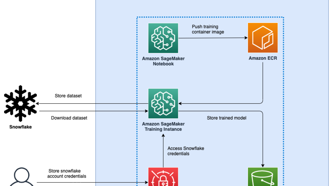
SageMaker Snowflake Architecture

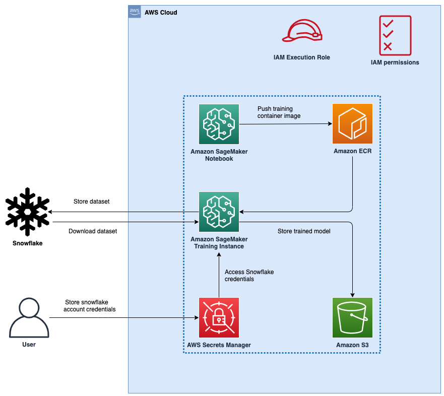
Figure 1: Architecture

The following figure represents the high-level architecture of the proposed solution to use Snowflake as a data source to train ML models with SageMaker.

The workflow steps are as follows:

  1. Set up a SageMaker notebook and an AWS Identity and Access Management (IAM) role with appropriate permissions to allow SageMaker to access Amazon Elastic Container Registry (Amazon ECR), Secrets Manager, and other services within your AWS account.
  2. Store your Snowflake account credentials in AWS Secrets Manager.
  3. Ingest the data in a table in your Snowflake account.
  4. Create a custom container image for ML model training and push it to Amazon ECR.
  5. Launch a SageMaker Training job for training the ML model. The training instance retrieves Snowflake credentials from Secrets Manager and then uses these credentials to download the dataset from Snowflake directly. This is the step that eliminates the need for data to be first downloaded into an S3 bucket.
  6. The trained ML model is stored in an S3 bucket.

Prerequisites

To implement the solution provided in this post, you should have an AWS account, a Snowflake account and familiarity with SageMaker.

Set up a SageMaker Notebook and IAM role

We use AWS CloudFormation to create a SageMaker notebook called aws-aiml-blogpost-sagemaker-snowflake-example and an IAM role called SageMakerSnowFlakeExample. Choose Launch Stack for the Region you want to deploy resources to.

AWS Region Link
us-east-1 (N. Virginia)
us-east-2 (Ohio)
us-west-1 (N. California)
us-west-2 (Oregon)
eu-west-1 (Dublin)
ap-northeast-1 (Tokyo)

Store Snowflake credentials in Secrets Manager

Store your Snowflake credentials as a secret in Secrets Manager. For instructions on how to create a secret, refer to Create an AWS Secrets Manager secret.

  1. Name the secret snowflake_credentials. This is required because the code in snowflake-load-dataset.ipynb expects the secret to be called that.
  2. Create the secret as a key-value pair with two keys:
    • username – Your Snowflake user name.
    • password – The password associated with your Snowflake user name.

Ingest the data in a table in your Snowflake account

To ingest the data, complete the following steps:

  1. On the SageMaker console, choose Notebooks in the navigation pane.
  2. Select the notebook aws-aiml-blogpost-sagemaker-snowflake-example and choose Open JupyterLab.

    Figure 2: Open JupyterLab

    Figure 2: Open JupyterLab

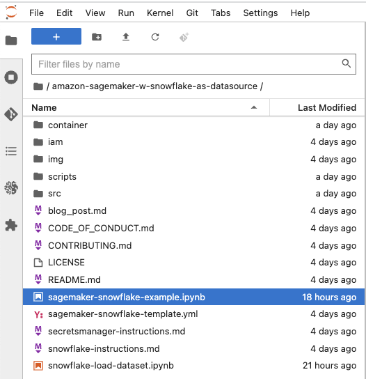
  3. Choose snowflake-load-dataset.ipynb to open it in JupyterLab. This notebook will ingest the California Housing Dataset to a Snowflake table.
  4. In the notebook, edit the contents of the following cell to replace the placeholder values with the one matching your snowflake account:
    sf_account_id = "your-snowflake-account-id"

  5. On the Run menu, choose Run All Cells to run the code in this notebook. This will download the dataset locally into the notebook and then ingest it into the Snowflake table.

    Figure 3: Notebook Run All Cells

    Figure 3: Notebook Run All Cells

The following code snippet in the notebook ingests the dataset into Snowflake. See the snowflake-load-dataset.ipynb notebook for the full code.

# connect to Snowflake Table schema
conn.cursor().execute(f"CREATE SCHEMA IF NOT EXISTS {schema}")
conn.cursor().execute(f"USE SCHEMA {schema}")

create_table_sql = f"CREATE TABLE IF NOT EXISTS {db}.{schema}.{table}n ("

california_housing.rename(columns=str.upper, inplace=True)
# iterating through the columns
for col in california_housing.columns:
    column_name = col.upper()

if (california_housing[col].dtype.name == "int" or california_housing[col].dtype.name == "int64"):
    create_table_sql = create_table_sql + column_name + " int"
elif california_housing[col].dtype.name == "object":
    create_table_sql = create_table_sql + column_name + " varchar(16777216)"
elif california_housing[col].dtype.name == "datetime64[ns]":
    create_table_sql = create_table_sql + column_name + " datetime"
elif california_housing[col].dtype.name == "float64":
    create_table_sql = create_table_sql + column_name + " float8"
elif california_housing[col].dtype.name == "bool":
    create_table_sql = create_table_sql + column_name + " boolean"
else:
    create_table_sql = create_table_sql + column_name + " varchar(16777216)"

# Deciding next steps. Either column is not the last column (add comma) else end create_tbl_statement
if california_housing[col].name != california_housing.columns[-1]:
    create_table_sql = create_table_sql + ",n"
else:
    create_table_sql = create_table_sql + ")"

# execute the SQL statement to create the table
print(f"create_table_sql={create_table_sql}")
conn.cursor().execute(create_table_sql)  
print(f"snowflake_table={snowflake_table}")
conn.cursor().execute('TRUNCATE TABLE IF EXISTS ' + snowflake_table)
  1. Close the notebook after all cells run without any error. Your data is now available in Snowflake. The following screenshot shows the california_housing table created in Snowflake.

    Figure 4: Snowflake Table

    Figure 4: Snowflake Table

Run the sagemaker-snowflake-example.ipynb notebook

This notebook creates a custom training container with a Snowflake connection, extracts data from Snowflake into the training instance’s ephemeral storage without staging it in Amazon S3, and performs Distributed Data Parallel (DDP) XGBoost model training on the data. DDP training is not required for model training on such a small dataset; it is included here for illustration of yet another recently released SageMaker feature.

Figure 5: Open SageMaker Snowflake Example Notebook

Figure 5: Open SageMaker Snowflake Example Notebook

Create a custom container for training

We now create a custom container for the ML model training job. Note that root access is required for creating a Docker container. This SageMaker notebook was deployed with root access enabled. If your enterprise organization policies don’t allow root access to cloud resources, you may want to use the following Docker file and shell scripts to build a Docker container elsewhere (for example, your laptop) and then push it to Amazon ECR. We use the container based on the SageMaker XGBoost container image 246618743249.dkr.ecr.us-west-2.amazonaws.com/sagemaker-xgboost:1.5-1 with the following additions:

  • The Snowflake Connector for Python to download the data from the Snowflake table to the training instance.
  • A Python script to connect to Secrets Manager to retrieve Snowflake credentials.

Using the Snowflake connector and Python script ensures that users who use this container image for ML model training don’t have to write this code as part of their training script and can use this functionality that is already available to them.

The following is the Dockerfile for the training container:

# Build an image that can be used for training in Amazon SageMaker, we use
# the SageMaker XGBoost as the base image as it contains support for distributed
# training.
FROM 246618743249.dkr.ecr.us-west-2.amazonaws.com/sagemaker-xgboost:1.5-1

MAINTAINER Amazon AI <sage-learner@amazon.com>

RUN apt-get -y update && apt-get install -y --no-install-recommends 
         wget 
         python3-pip 
         python3-setuptools 
         nginx 
         ca-certificates 
   && rm -rf /var/lib/apt/lists/*

RUN ln -s /usr/bin/python3 /usr/bin/python
RUN ln -s /usr/bin/pip3 /usr/bin/pip

# Here we get snowflake-connector python package.
# pip leaves the install caches populated which uses a 
# significant amount of space. These optimizations save a fair 
# amount of space in the image, which reduces start up time.
RUN pip --no-cache-dir install snowflake-connector-python==2.8.3  

# Include python script for retrieving Snowflake credentials 
# from AWS SecretsManager
ADD snowflake_credentials.py /

The container image is built and pushed to Amazon ECR. This image is used for training the ML model.

Train the ML model using a SageMaker Training job

After we successfully create the container image and push it to Amazon ECR, we can start using it for model training.

  1. We create a set of Python scripts to download the data from Snowflake using the Snowflake Connector for Python, prepare the data and then use the XGBoost Regressor to train the ML model. It is the step of downloading the data directly to the training instance that avoids having to use Amazon S3 as the intermediate storage for training data.
  2. We facilitate Distributed Data Parallel training by having the training code download a random subset of the data such that each training instance downloads an equal amount of data from Snowflake. For example, if there are two training nodes, then each node downloads a random sample of 50% of the rows in the Snowflake table.See the following code:
    """
    Read the HOUSING table (this is the california housing dataset  used by this example)
    """
    import pandas as pd
    import snowflake.connector
    
    def data_pull(ctx: snowflake.connector.SnowflakeConnection, table: str, hosts: int) -> pd.DataFrame:
    
        # Query Snowflake HOUSING table for number of table records
        sql_cnt = f"select count(*) from {table};"
        df_cnt = pd.read_sql(sql_cnt, ctx)
    
        # Retrieve the total number of table records from dataframe
        for index, row in df_cnt.iterrows():
            num_of_records = row.astype(int)
            list_num_of_rec = num_of_records.tolist()
        tot_num_records = list_num_of_rec[0]
    
        record_percent = str(round(100/hosts))
        print(f"going to download a random {record_percent}% sample of the data")
        # Query Snowflake HOUSING table
        sql = f"select * from {table} sample ({record_percent});"
        print(f"sql={sql}")
    
        # Get the dataset into Pandas
        df = pd.read_sql(sql, ctx)
        print(f"read data into a dataframe of shape {df.shape}")
        # Prepare the data for ML
        df.dropna(inplace=True)
    
        print(f"final shape of dataframe to be used for training {df.shape}")
        return df

  3. We then provide the training script to the SageMaker SDK Estimator along with the source directory so that all the scripts we create can be provided to the training container when the training job is run using the Estimator.fit method:
    custom_img_uri = f"{account_id}.dkr.ecr.{region}.amazonaws.com/{custom_img_name}:{custom_img_tag}"
    
    # Create Sagemaker Estimator
    xgb_script_mode_estimator = sagemaker.estimator.Estimator(
        image_uri = custom_img_uri,
        role=role,
        instance_count=instance_count,
        instance_type=instance_type,
        output_path="s3://{}/{}/output".format(bucket, prefix),
        sagemaker_session=session,
        entry_point="train.py",
        source_dir="./src",
        hyperparameters=hyperparams,
        environment=env,
        subnets = subnet_ids,
    )
    
    # start the training job
    xgb_script_mode_estimator.fit()

    For more information, refer to Prepare a Scikit-Learn Training Script.

  4. After the model training is complete, the trained model is available as a model.tar.gz file in the default SageMaker bucket for the Region:
print(f"the trained model is available in Amazon S3 -> {xgb_script_mode_estimator.model_data}")

You can now deploy the trained model for getting inference on new data! For instructions, refer to Create your endpoint and deploy your model.

Clean up

To avoid incurring future charges, delete the resources. You can do this by deleting the CloudFormation template used to create the IAM role and SageMaker notebook.

Figure 6: Cleaning Up

You will have to delete the Snowflake resources manually from the Snowflake console.

Conclusion

In this post, we showed how to download data stored in a Snowflake table to a SageMaker Training job instance and train an XGBoost model using a custom training container. This approach allows us to directly integrate Snowflake as a data source with a SageMaker notebook without having the data staged in Amazon S3.

We encourage you to learn more by exploring the Amazon SageMaker Python SDK and building a solution using the sample implementation provided in this post and a dataset relevant to your business. If you have questions or suggestions, leave a comment.


About the authors

Amit Arora is an AI and ML specialist architect at Amazon Web Services, helping enterprise customers use cloud-based machine learning services to rapidly scale their innovations. He is also an adjunct lecturer in the MS data science and analytics program at Georgetown University in Washington D.C.

Divya Muralidharan is a Solutions Architect at Amazon Web Services. She is passionate about helping enterprise customers solve business problems with technology. She has a Masters in Computer Science from Rochester Institute of Technology. Outside of office, she spends time cooking, singing, and growing plants.

Sergey Ermolin is a Principal AIML Solutions Architect at AWS. Previously, he was a software solutions architect for deep learning, analytics, and big data technologies at Intel. A Silicon Valley veteran with a passion for machine learning and artificial intelligence, Sergey has been interested in neural networks since pre-GPU days, when he used them to predict aging behavior of quartz crystals and cesium atomic clocks at Hewlett-Packard. Sergey holds an MSEE and a CS certificate from Stanford and a BS degree in physics and mechanical engineering from California State University, Sacramento. Outside of work, Sergey enjoys wine-making, skiing, biking, sailing, and scuba-diving. Sergey is also a volunteer pilot for Angel Flight.
Read More

How Marubeni is optimizing market decisions using AWS machine learning and analytics

How Marubeni is optimizing market decisions using AWS machine learning and analytics

This post is co-authored with Hernan Figueroa, Sr. Manager Data Science at Marubeni Power International.

Marubeni Power International Inc (MPII) owns and invests in power business platforms in the Americas. An important vertical for MPII is asset management for renewable energy and energy storage assets, which are critical to reduce the carbon intensity of our power infrastructure. Working with renewable power assets requires predictive and responsive digital solutions, because renewable energy generation and electricity market conditions are continuously changing. MPII is using a machine learning (ML) bid optimization engine to inform upstream decision-making processes in power asset management and trading. This solution helps market analysts design and perform data-driven bidding strategies optimized for power asset profitability.

In this post, you will learn how Marubeni is optimizing market decisions by using the broad set of AWS analytics and ML services, to build a robust and cost-effective Power Bid Optimization solution.

Solution overview

Electricity markets enable trading power and energy to balance power supply and demand in the electric grid and to cover different electric grid reliability needs. Market participants, such as MPII asset operators, are constantly bidding power and energy quantities into these electricity markets to obtain profits from their power assets. A market participant can submit bids to different markets simultaneously to increase the profitability of an asset, but it needs to consider asset power limits and response speeds as well as other asset operational constraints and the interoperability of those markets.

MPII’s bid optimization engine solution uses ML models to generate optimal bids for participation in different markets. The most common bids are day-ahead energy bids, which should be submitted 1 day in advance of the actual trading day, and real-time energy bids, which should be submitted 75 minutes before the trading hour. The solution orchestrates the dynamic bidding and operation of a power asset and requires using optimization and predictive capabilities available in its ML models.

The Power Bid Optimization solution includes multiple components that play specific roles. Let’s walk through the components involved and their respective business function.

Data collection and ingestion

The data collection and ingestion layer connects to all upstream data sources and loads the data into the data lake. Electricity market bidding requires at least four types of input:

  • Electricity demand forecasts
  • Weather forecasts
  • Market price history
  • Power price forecasts

These data sources are accessed exclusively through APIs. Therefore, the ingestion components need to be able to manage authentication, data sourcing in pull mode, data preprocessing, and data storage. Because the data is being fetched hourly, a mechanism is also required to orchestrate and schedule ingestion jobs.

Data preparation

As with most ML use cases, data preparation plays a critical role. Data comes from disparate sources in a number of formats. Before it’s ready to be consumed for ML model training, it must go through some of the following steps:

  • Consolidate hourly datasets based on time of arrival. A complete dataset must include all sources.
  • Augment the quality of the data by using techniques such as standardization, normalization, or interpolation.

At the end of this process, the curated data is staged and made available for further consumption.

Model training and deployment

The next step consists of training and deploying a model capable of predicting optimal market bids for buying and selling energy. To minimize the risk of underperformance, Marubeni used the ensemble modeling technique. Ensemble modeling consists of combining multiple ML models to enhance prediction performance. Marubeni ensembles the outputs of external and internal prediction models with a weighted average to take advantage of the strength of all models. Marubeni’s internal models are based on Long Short-Term Memory (LSTM) architectures, which are well documented and easy to implement and customize in TensorFlow. Amazon SageMaker supports TensorFlow deployments and many other ML environments. The external model is proprietary, and its description cannot be included in this post.

In Marubeni’s use case, the bidding models perform numerical optimization to maximize the revenue using a modified version of the objective functions used in the publication Opportunities for Energy Storage in CAISO.

SageMaker enables Marubeni to run ML and numerical optimization algorithms in a single environment. This is critical, because during the internal model training, the output of the numerical optimization is used as part of the prediction loss function. For more information on how to address numerical optimization use cases, refer to Solving numerical optimization problems like scheduling, routing, and allocation with Amazon SageMaker Processing.

We then deploy those models through inference endpoints. As fresh data is ingested periodically, the models need to be retrained because they become stale over time. The architecture section later in this post provides more details on the models’ lifecycle.

Power bid data generation

On an hourly basis, the solution predicts the optimal quantities and prices at which power should be offered on the market—also called bids. Quantities are measured in MW and prices are measured in $/MW. Bids are generated for multiple combinations of predicted and perceived market conditions. The following table shows an example of the final bid curve output for operating hour 17 at an illustrative trading node near Marubeni’s Los Angeles office.

Date Hour Market Location MW Price
11/7/2022 17 RT Energy LCIENEGA_6_N001 0 $0
11/7/2022 17 RT Energy LCIENEGA_6_N001 1.65 $80.79
11/7/2022 17 RT Energy LCIENEGA_6_N001 5.15 $105.34
11/7/2022 17 RT Energy LCIENEGA_6_N001 8 $230.15

This example represents our willingness to bid 1.65 MW of power if the power price is at least $80.79, 5.15 MW if the power price is at least $105.34, and 8 MW if the power price is at least $230.15.

Independent system operators (ISOs) oversee electricity markets in the US and are responsible for awarding and rejecting bids to maintain electric grid reliability in the most economical way. California Independent System Operator (CAISO) operates electricity markets in California and publishes market results every hour prior to the next bidding window. By cross-referencing current market conditions with their equivalent on the curve, analysts are able to infer optimal revenue. The Power Bid Optimization solution updates future bids using new incoming market information and new model predictive outputs

AWS architecture overview

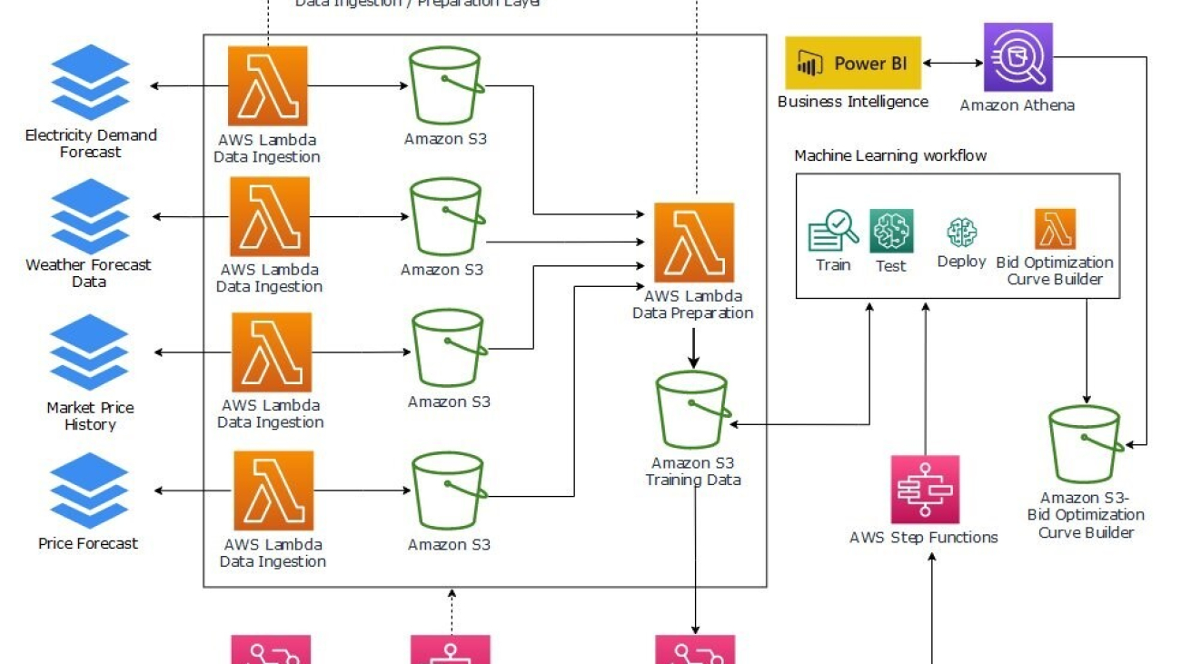
The solution architecture illustrated in the following figure implements all the layers presented earlier. It uses the following AWS services as part of the solution:

  • Amazon Simple Storage Service (Amazon S3) to store the following data:
    • Pricing, weather, and load forecast data from various sources.
    • Consolidated and augmented data ready to be used for model training.
    • Output bid curves refreshed hourly.
  • Amazon SageMaker to train, test, and deploy models to serve optimized bids through inference endpoints.
  • AWS Step Functions to orchestrate both the data and ML pipelines. We use two state machines:
    • One state machine to orchestrate data collection and ensure that all sources have been ingested.
    • One state machine to orchestrate the ML pipeline as well as the optimized bidding generation workflow.
  • AWS Lambda to implement ingestion, preprocessing, and postprocessing functionality:
    • Three functions to ingest input data feeds, with one function per source.
    • One function to consolidate and prepare the data for training.
    • One function that generates the price forecast by calling the model’s endpoint deployed within SageMaker.
  • Amazon Athena to provide developers and business analysts SQL access to the generated data for analysis and troubleshooting.
  • Amazon EventBridge to trigger the data ingestion and ML pipeline on a schedule and in response to events.

Solution Architecture Diagram
In the following sections, we discuss the workflow in more detail.

Data collection and preparation

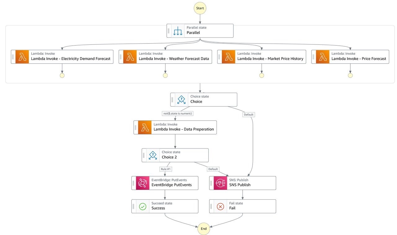
Every hour, the data preparation Step Functions state machine is invoked. It calls each of the data ingestion Lambda functions in parallel, and waits for all four to complete. The data collection functions call their respective source API and retrieve data for the past hour. Each function then stores the received data into their respective S3 bucket.

These functions share a common implementation baseline that provides building blocks for standard data manipulation such as normalization or indexation. To achieve this, we use Lambda layers and AWS Chalice, as described in Using AWS Lambda Layers with AWS Chalice. This ensures all developers are using the same base libraries to build new data preparation logics and speeds up implementation.

Data Ingestion and Preparation State Machine

After all four sources have been ingested and stored, the state machine triggers the data preparation Lambda function. Power price, weather, and load forecast data is received in JSON and character delimited files. Each record part of each file carries a timestamp that is used to consolidate data feeds into one dataset covering a time frame of 1 hour.

This construct provides a fully event-driven workflow. Training data preparation is initiated as soon as all the expected data is ingested.

ML pipeline

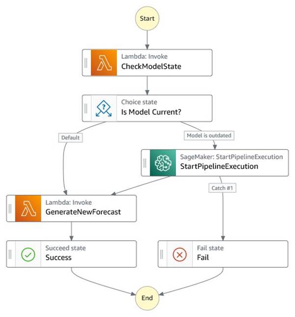
After data preparation, the new datasets are stored into Amazon S3. An EventBridge rule triggers the ML pipeline through a Step Functions state machine. The state machine drives two processes:

  • Check if the bid curve generation model is current
  • Automatically trigger model retraining when performance degrades or models are older than a certain amount of days

If the age of the currently deployed model is older than the latest dataset by a certain threshold—say 7 days—the Step Functions state machine kicks off the SageMaker pipeline that trains, tests, and deploys a new inference endpoint. If the models are still up to date, the workflow skips the ML pipeline and moves on to the bid generation step. Regardless of the state of the model, a new bid curve is generated upon delivery of a new hourly dataset. The following diagram illustrates this workflow. By default, the StartPipelineExecution action is asynchronous. We can have the state machine wait for the end of the pipeline before invoking the bids generation step by using the ‘Wait-for callback‘ option.

Bid Curve Generation State Machine

Step Functions Wait For Callback Option

To reduce cost and time to market in building a pilot solution, Marubeni used Amazon SageMaker Serverless Inference. This ensures that the underlying infrastructure used for training and deployment incurs charges only when needed. This also makes the process of building the pipeline easier because developers no longer need to manage the infrastructure. This is a great option for workloads that have idle periods between traffic spurts. As the solution matures and transitions into production, Marubeni will review their design and adopt a configuration more suited for predictable and steady usage.

Bids generation and data querying

The bids generation Lambda function periodically invokes the inference endpoint to generate hourly predictions and stores the output into Amazon S3.

Developers and business analysts can then explore the data using Athena and Microsoft Power BI for visualization. The data can also be made available via API to downstream business applications. In the pilot phase, operators visually consult the bid curve to support their power transaction activities on markets. However, Marubeni is considering automating this process in the future, and this solution provides the necessary foundations to do so.

Conclusion

This solution enabled Marubeni to fully automate their data processing and ingestion pipelines as well as reduce their predictive and optimization models’ deployment time from hours to minutes. Bid curves are now automatically generated and kept up to date as market conditions change. They also realized an 80% cost reduction when switching from a provisioned inference endpoint to a serverless endpoint.

MPII’s forecasting solution is one of the recent digital transformation initiatives Marubeni Corporation is launching in the power sector. MPII plans to build additional digital solutions to support new power business platforms. MPII can rely on AWS services to support their digital transformation strategy across many use cases.

We can focus on managing the value chain for new business platforms, knowing that AWS is managing the underlying digital infrastructure of our solutions.

– Hernan Figueroa, Sr. Manager Data Science at Marubeni Power International.

For more information on how AWS is helping energy organizations in their digital transformation and sustainability initiatives, refer to AWS Energy.

Marubeni Power International is a subsidiary of Marubeni Corporation. Marubeni Corporation is a major Japanese trading and investment business conglomerate.  Marubeni Power International mission is to develop new business platforms, assess new energy trends and technologies and manage Marubeni’s power portfolio in the Americas. If you would like to know more about Marubeni Power, check out https://www.marubeni-power.com/.


About the Authors

Hernan Figueroa leads the digital transformation initiatives at Marubeni Power International. His team applies data science and digital technologies to support Marubeni Power growth strategies. Before joining Marubeni, Hernan was a Data Scientist at Columbia University. He holds a Ph.D. in Electrical Engineering and a B.S. in Computer Engineering.

Lino Brescia is a Principal Account Executive based in NYC. He has over 25 years of technology experience and has joined AWS in 2018. He manages global enterprise customers as they transform their business with AWS cloud services and perform large-scale migrations.

Narcisse Zekpa is a Sr. Solutions Architect based in Boston. He helps customers in the Northeast U.S. accelerate their business transformation through innovative, and scalable solutions, on the AWS Cloud. When Narcisse is not building, he enjoys spending time with his family, traveling, cooking, playing basketball, and running.

Pedram Jahangiri is an Enterprise Solution Architect with AWS, with a PhD in Electrical Engineering. He has 10+ years experience in the energy and IT industry. Pedram has many years of hands-on experience in all aspects of Advanced Analytics for building quantitative and large-scale solutions for enterprises by leveraging cloud technologies.

Sarah Childers is an Account Manager based in Washington DC. She is a former science educator turned cloud enthusiast focused on supporting customers through their cloud journey. Sarah enjoys working alongside a motivated team that encourages diversified ideas to best equip customers with the most innovative and comprehensive solutions.
Read More

Portfolio optimization through multidimensional action optimization using Amazon SageMaker RL

Portfolio optimization through multidimensional action optimization using Amazon SageMaker RL

Reinforcement learning (RL) encompasses a class of machine learning (ML) techniques that can be used to solve sequential decision-making problems. RL techniques have found widespread applications in numerous domains, including financial services, autonomous navigation, industrial control, and e-commerce. The objective of an RL problem is to train an agent that, given an observation from its environment, will choose the optimal action that maximizes cumulative reward. Solving a business problem with RL involves specifying the agent’s environment, the space of actions, the structure of observations, and the right reward function for the target business outcome. In policy-based RL methods, the outcome of model training is often a policy, which defines a probability distribution over the actions given an observation. The optimal policy will maximize the cumulative returns obtained by the agent.

In constrained decision-making problems, the agent is tasked with choosing the optimal actions under constraints. A distinct class of such problems exists wherein, depending on the state, the agent may be only allowed to choose from a subset of all actions. The remaining actions are inadmissible.

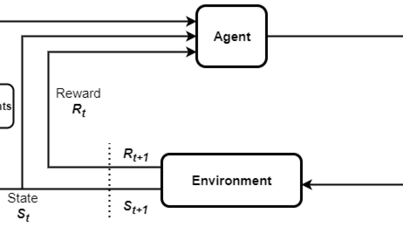
For example, consider an autonomous car that has 10 possible speed levels. This car may only be allowed to choose from a subset of its speed levels when traversing a residential neighborhood. Here, the constraint on the speed levels is determined by the location of the car. Such parameterized constraints on the actions are common in many real-world problems. Solving such problems with RL requires incorporating the constraints in the training process. Action masking is an approach to solve RL problems that involve inadmissibility constraints in a sample efficient manner. As the name suggests, it involves masking any inadmissible actions by setting their sampling probability to zero. The following figure depicts the RL cycle with action masking. It consists of an agent, the constraints that determine the action masks, the masks, state transitions, and the observed rewards.

In this post, we describe how to implement action masking with Amazon SageMaker RL using parametric action spaces in Ray RLlib. We describe an example problem that involves discrete multidimensional action spaces and multiple constraints. To access the complete notebook for this post, see the SageMaker notebook example on GitHub.

Use case overview

We consider an example portfolio optimization problem in which an investor trades multiple asset types to maximize their total portfolio value. The portfolio consists of three different asset types, and a cash balance that simply refers to money you have in your bank account. During each investment period, the agent has to choose the quantity of each asset type that they buy or sell. The agent uses the available cash balance to finance any asset purchases. There are also transactions costs associated with each asset buy/sell action. The market price of each asset is assumed to vary across time. The prices are sampled randomly but modeled to show distinct behavior with different levels of volatility. The price ranges for the three asset classes are shown in the following figure.

The set of admissible actions for the agent are determined by parameters such as the current total portfolio value, current cash balance, the number of each types of assets held, and their current market value. For this problem, we enforce the following constraints on possible actions:

  • C1 – The agent can’t sell more units of any asset type than what they currently own. For example, if the agent has 100 units of Asset 3 at time k in their portfolio, then it can’t sell 120 units of that asset at that time.
  • C2 – Asset 3 is considered highly volatile by investors. The agent is not allowed to buy Asset 3 if the total value of their holdings in Asset 3 is above a third of their total portfolio value.
  • C3 – Consumers of the RL model have a moderate risk preference and consider Asset 2 a conservative buy. As a result, the agent is not allowed to buy Asset 2 when the total value of Asset 2 holdings cross two-thirds of the total portfolio value.
  • C4 – The agent can’t buy any assets if its current cash balance is less than $1 USD.

Set up the environment

To start, provision a SageMaker notebook instance via Amazon SageMaker Studio. For more information, see Use Amazon SageMaker Notebook instances.

Next, we implement the portfolio trading problem in a custom Open AI Gym environment and train an RL agent using SageMaker RL. A Gym environment provides an interface for the RL agent to interact with its environment, and to generate rewards and observations. The environment for the portfolio trading is located in the trading.py module. We use the __init__ method to define and initialize some environment parameters. This includes transaction costs associated with asset buy/sell actions, mean value of the asset prices, price variances, and more. We also define the observation and action spaces in the __init__ method. See the following code:

def __init__(self,*args, **kwargs): 

        self.buy_price=np.array([0.03, 0.045, 0.035]) # transaction cost per unit bought for three asset classes
        self.sell_price=np.array([0.025, 0.035, 0.03]) # transaction cost per unit sold for three asset classes
        self.mu=np.array([40,35,48])                         # Mean initial asset price
        self.var=np.array([4,2,7])                           # Variance of asset prices
        self.tvec=np.arange(20)                              # Length of each episode=20
        self.sig=np.zeros((3,len(self.tvec)))
        self.sig[0,:]=self.mu[0]+0.4*self.tvec+4*np.cos(2*math.pi*self.tvec/16)  #Functions used to model mean asset prices over time
        self.sig[1,:]=self.mu[1]+0.1*self.tvec
        self.sig[2,:]=self.mu[2]+0.3*self.tvec-6*np.sin(2*math.pi*self.tvec/7)
        
        state_bounds=state_bounds_gen()
        low,high= map(np.array,zip(*state_bounds.values()))  # Minimum and maximum values for the state variables         
        
        self.action_space = Tuple([Discrete(11),Discrete(11),Discrete(11)])  #Action space consisting of three discrete actions
        
        self.observation_space=Dict({"action_mask":Tuple([Box(0,1,shape=(11,)),Box(0,1,shape=(11,)),Box(0,1,shape=(11,))]),
                                     "trading_state":Box(low,high,dtype=np.float32)})  # Dictionary space consisting of trading state 
                                                                                       # and action mask

Because the agent trades three assets at any given time, the actions taken by the agent are represented using a three-dimensional action vector. The three discrete actions that make up the action vector represent the trades in each asset classes and can each take 11 possible values. The 11 discrete values encode different sell, buy, and hold actions, as shown in the following figure. For example, choosing a1=3 translates to the agent selling 20 units of the asset type 1. Assets are bought and sold in multiples of 10.

The observation space has a dictionary structure with two elements. These represent the current trading state and the current action mask values. The trading state is a 7×1 vector consisting of the quantities of each assets currently held by the agent, current cash balance, and the current market value of each of the three assets. The action mask is a 3×11 matrix with mask values corresponding to each possible action. The environment calculates the mask values at every time using an update_mask() method. Actions that violate any of the constraints C1:C4 are assigned a zero mask. The value of mask is set to be 1 for admissible actions. See the following code:

def update_mask(self):
        
        self.action_mask=[np.array([1.0]*x.n) for x in self.action_space.spaces]  # Set all masks to 1 
       
        if self.balance<1:                                                        # If balance < 1, set buy masks to zero (C4)
            for jj in range(len(self.action_mask)):
                self.action_mask[jj][6:]=[0.0]*5
           
        self.action_mask[2][6:]=[0.0]*5 if (self.prices[2]*self.assets[2]/self.total_assets)>1.0/3.0 else [1.0]*5  #(C3)
        
        self.action_mask[1][6:]=[0.0]*5 if (self.prices[1]*self.assets[1]/self.total_assets)>2.0/3.0 else [1.0]*5  #(C2)
        
        for k in range(3):
            cap=int(min(5,self.assets[k]/10))
            self.action_mask[k][:5]=[0.0]*(5-cap)+[1.0]*cap                                          # (C1)

At the beginning of each episode, a reset() method is called to reinitialize the trading state, observations, and other parameters. The agent starts each training episode with $1,000 USD in cash balance and zero holdings in assets. Each episode consists of 20 investment periods.

 def reset(self):
        
        self.assets=np.zeros(3,dtype=np.float32) # Assets owned at the beginning
        self.balance=1000                               # Initial cash balance
        self.t_step=0
        self.prices=[np.random.normal(mu,var) for mu,var in zip(self.mu,self.var)]  # Sampling market prices for the assets
        self.state=np.hstack([self.assets, self.balance, self.prices])        # Initial state
        self.total_assets=self.balance               # Total portfolio value
        self.update_mask()                         # Updating action mask values
        
        reset_state={
            "action_mask":list(np.float32(self.action_mask)),    # Initial state  
            "trading_state":np.float32(self.state)
        }
        
        return reset_state

At the beginning of every investment period, the agent samples an action based on the latest observations it recorded and updates its portfolio. This is modeled using a step() method. After the portfolio is updated, we recalculate the state. The action mask is also updated by calling the update_mask() method.

def step(self, action):    
        self.t_step+=1
        
        for index, a in enumerate (action):
            print("action is ",a)
            print("price is ",self.prices[index])
            quant=abs(a-5)                                              # Number of assets traded/10
            if a<5:                                                     # Condition: Asset sale ?
                if 10*quant*self.sell_price[index]>self.balance:        # Condition: sale cost > Balance ? 
                    quant=np.floor(self.balance/(10*self.sell_price[index]))    
                self.assets[index]-=10*quant                               # Asset update
                self.balance=self.balance+10*quant*(self.prices[index]-self.sell_price[index]) # Balance update
            if a>5:
                if 10*quant*(self.buy_price[index]+self.prices[index])>self.balance:          # Condition: Buy cost > Balance ?
                    quant=np.floor(self.balance/(10*(self.buy_price[index]+self.prices[index])))
                self.assets[index]+=10*quant                               # Asset update
                self.balance=self.balance-10*quant*(self.prices[index]+self.sell_price[index]) # Balance update
            else:
                continue
        
        self.prices=np.array([np.random.normal(mu,var) for mu,var in zip(self.sig[:,self.t_step],self.var)]) # New asset prices
        self.state=np.hstack([self.assets,self.balance, self.prices])                                        # New state
        self.total_assets=self.balance+np.dot(self.assets,self.prices)                                       # Total portfolio value
        self.update_mask()                                                                                   # Mask update
       
        obs={
            "action_mask": list(np.float32(self.action_mask)),
            "trading_state":np.float32(self.state)
            
        }
       
        if self.t_step==len(self.tvec)-1:
            reward=self.total_assets        # reward = Total portfolio value at the end of the episode
        else:
            reward=0
        done=True if self.t_step==len(self.tvec)-1 else False
        return obs, reward, done, {}

The reward function is defined as the final total portfolio value and calculated at the end of each episode, which happens after 20 investment periods.

Masking model

At each time step, the environment returns the dictionary state and the ML model representing the policy samples an action based on this state. A parametric action model facilitates sampling only the unmasked (mask ≠ 0) actions. Here we describe the parametric actions model that enables action masking:

class ParametricActionsModel(TFModelV2):
    
    def __init__(self, obs_space, action_space, num_outputs,
        model_config, name, *args, **kwargs):
        
        super(ParametricActionsModel, self).__init__(obs_space,
            action_space, num_outputs, model_config, name, *args, **kwargs)
        
        self.true_obs_shape = (7,)

        self.action_embed_model = FullyConnectedNetwork(Box(np.finfo(np.float32).min,np.finfo(np.float32).max,shape=self.true_obs_shape),
                                  action_space,
                                  num_outputs,
                                  model_config,
                                  name,
                                                       )             # action embedding model
        self.register_variables(self.action_embed_model.variables())
        
    
    def forward(self, input_dict, state, seq_lens):
        
        action_mask= tf.cast(tf.concat(input_dict["obs"]["action_mask"], axis=1), tf.float32)  # action mask values
        
        action_embedding,_ = self.action_embed_model({"obs":input_dict["obs"]["trading_state"]}) # action embeddings
        
        logit_mod = tf.maximum(tf.math.log(action_mask),tf.float32.min)                          # moidfiers to action logits
        
        return (action_embedding+logit_mod), state
    
    def value_function(self):
        return self.action_embed_model.value_function()

Actions are sampled by the model through a Softmax function using the logits given by an action embedding model. This model is defined in the __init__ method. The masking behavior itself is implemented in the forward() method. Here, we separate the actions masks and trading state from the dictionary state retrieved from the environment. The action embeddings are then obtained by passing the trading state to the action embedding network. Next, we modify the value of embeddings of each action by adding logit_mod to the logits. Notice that logit_mod is a function of the logarithm of the action mask. For actions with mask =1, the logarithm of mask will be zero, which leaves their embeddings unperturbed. On the other hand, when mask=0, the logarithm of mask → −∞. Because Softmax(x) →0 as x→ −∞, this makes sure that masked actions aren’t sampled by the agent.

Let’s test if the mask is working as expected. We initiate a ray trainer object and mask some of the actions and see if the trainer is sampling only the unmasked actions:

import ray
import ray.rllib.agents.ppo as ppo
from ray.tune.registry import register_env
from trading import mytradingenv
from mask_model import register_actor_mask_model
import numpy as np

register_actor_mask_model()
ray.shutdown()
ray.init(ignore_reinit_error=True)

env_config={}
register_env("customtradingmodel", lambda env_config:mytradingenv(env_config))

TestEnvConfig = {
    "log_level":"WARN",

        "model": {
                      
            "custom_model": "trading_mask"        # Define the custom masking model in the config                  
                            
            
            }
        }

agent1 = ppo.PPOTrainer(config=TestEnvConfig,env="customtradingmodel")
env = agent1.env_creator('customtradingmodel')
state=env.reset()
print(state["action_mask"])

The output in the following screenshot shows the initial action mask array.

Now we modify the mask vectors so that for a1, all choices except action 8 (buy 30 units of Asset 1); for a2 everything except action 5 (hold Asset 2 at current numbers); and for a3, everything except actions 1 and 2 (sell 40 or 30 units of Asset 3) are masked:

state["action_mask"]=[np.zeros([11],dtype=np.float32) for _ in range(3)]
state['action_mask'][0][8]=1
state['action_mask'][1][5]=1
state['action_mask'][2][1:3]=[1,1]

Now that we have modified the action mask array, we try and sample a new action.

The agent samples only those actions that are unmasked. This verifies that action masking is working as expected.

Results

Now that the environment and parametric actions model are defined, we train an agent to solve the portfolio optimization problem using SageMaker RL. We train an RL agent to learn the optimal policy to maximize the reward under the constraints C1:C4. We use the proximal policy optimization (PPO) algorithm in SageMaker RL to train the RL agent for 500,000 episodes. The following training configuration shows how we specify the agent to use the trading_mask as a custom_model to be used:

    def get_experiment_config(self):
        return {
            "training": {
                   "env": "mytradingmodel",
                   "run": "PPO",                     # Use PPO algorithm
                   "stop":{"episodes_total":500000}, # 500k training episodes
                   "config": {
                      "use_pytorch": False,
                      "gamma": 0.99,
                      "kl_coeff": 1.0,
                      "num_sgd_iter": 20,
                      "lr": 0.0001,
                      "sgd_minibatch_size": 1000,
                      "train_batch_size": 25000,
                      "monitor": True,  
                      "model": {
                          "custom_model": "trading_mask"  # Use custom action masking model                        
                            },
                      "num_workers": (self.num_cpus-1),
                      "num_gpus": self.num_gpus,
                      "batch_mode": "truncate_episodes",
                       "explore":True,
                       "exploration_config":{
                           "type":"StochasticSampling",  
                       },
                     },
                     "checkpoint_freq": 1, 
                  }
             }

The agent starts with $1,000 USD in initial cash balance. The mean reward per episode is plotted as a function of training time, as shown in the following chart. Recall that we use the final total portfolio value as reward. At the end of 20 investment periods, we observe that the mean value of the agent’s portfolio is over $3,000 USD.

Clean up

We didn’t provision any infrastructure beyond the use of a SageMaker notebook instance. If you’re using a SageMaker notebook instance via Studio, you can shut it down by following the instructions in Shut Down an Open Notebook.

Conclusion

In this post, we discussed how you can implement action masking to enforce constraints in RL model training. By masking inadmissible actions, we enable the agent to sample only valid actions and learn the optimal policy in a sample efficient manner. We introduced a portfolio optimization problem wherein the agent is tasked with maximizing their portfolio value by trading three asset types under multiple constraints. We demonstrated how to implement multi-dimensional action masking for this problem using Ray RLlib. We trained an RL agent for solving the constrained portfolio optimization problem using SageMaker RL.

Now that you know how to perform action masking using SageMaker RL and Ray RLlib on portfolio optimization, you can try it on other RL problems that involve inadmissible actions. You can also adapt the action masking code developed in this post for simpler problems involving one-dimensional action space. We encourage you to apply the approach developed here to your RL use cases and let us know if you have any questions or feedback.

Additional references

For additional information and related content, see the following resources:


About the Authors

Dilshad Raihan Akkam Veettil is a Data Scientist with AWS Professional Services, where he engages with customers across industries to solve their business challenges through the use of machine learning and cloud computing. He holds a PhD in Aerospace Engineering from Texas A&M University, College Station. In his leisure time, he enjoys watching football and reading.

Paul Budnarain is an Applied Scientist in Amazon’s Inventory Forecasting Systems (IFS) group, and is based out of Los Angeles,California.

Read More