Achieving Zero-COGS with Microsoft Editor Neural Grammar Checker

Achieving Zero-COGS with Microsoft Editor Neural Grammar Checker

black male sitting at a table working on a laptop

Microsoft Editor provides AI-powered writing assistance to millions of users around the world. One of its features that writers of all levels and domains rely on is the grammar checker, which detects grammar errors in a user’s writing and offers suggested corrections and explanations of the detected errors.

The technology behind grammar checker has evolved significantly since the 1970s, when the first-generation tool was based on simple pattern matching. A major breakthrough occurred in 1997, when Microsoft Word 97 introduced a grammar checker that relied on a full-fledged natural language processing system (Heidorn, 2000), enabling more sophisticated and accurate error detection and correction. Another major breakthrough occurred in 2020, when Microsoft launched a neural grammar checker that leveraged deep neural networks with a novel fluency boost learning and inference mechanism, achieving state-of-the-art results on both CoNLL-2014 and JFLEG benchmark datasets[1,2]. In 2022, Microsoft released a highly optimized version of the Microsoft Editor neural grammar checker on expanded endpoints in Word Win32, Word Online, Outlook Online, and the Editor Browser Extension.

In this blog post, we will describe how we have optimized the Editor neural grammar checker model using the Aggressive Decoding algorithm pioneered by Microsoft Research (MSR) and accelerated with high performance ONNX Runtime (ORT). With the Aggressive Decoding algorithm and ORT optimizations, the server model has achieved ~200% increase in inference speed while saving two-thirds of the cost, with no loss of model prediction quality compared to the previous production model.

Spotlight: Microsoft Research Podcast

AI Frontiers: AI for health and the future of research with Peter Lee

Peter Lee, head of Microsoft Research, and Ashley Llorens, AI scientist and engineer, discuss the future of AI research and the potential for GPT-4 as a medical copilot.

But we did not stop there. We also implemented EdgeFormer, MSR’s cutting-edge on-device seq2seq modeling technology, to obtain a lightweight generative language model with competitive performance that can be run on a user’s device, allowing us to achieve the ultimate zero-cost-of-goods-sold (COGS) goal.

Shipping a client model offers three other key benefits in addition to achieving zero-COGS:

  1. Increased privacy. A client model that runs locally on the user’s device does not need to send any personal data to a remote server.
  2. Increased availability. A client model operates offline without relying on network connectivity, bandwidth, or server capacity.
  3. Reduced cost and increased scalability. Shipping a client model to a user’s device removes all the computation that a server would be required to execute, which allows us to ship to more customers.

Additionally, we leveraged GPT-3.5 (the most advanced AI model at the time) to generate high-quality training data and identify and remove low-quality training examples, leading to a boost of model performance.

Innovation: Aggressive Decoding

Behind the AI-powered grammar checker in Microsoft Editor is the transformer model, enhanced by cutting-edge research innovations[1,2,3] from MSR for grammar correction. As with most seq2seq tasks, we used autoregressive decoding for high-quality grammar correction. However, conventional autoregressive decoding is very inefficient as it cannot fully utilize modern computing devices (CPUs, GPUs) due to its low computational parallelism, which results in high model serving costs and prevents us from scaling quickly to more (web/desktop) endpoints.

To address the challenge for serving cost reduction, we adopt the latest decoding innovation, Aggressive Decoding,[3] published by MSR researchers Tao Ge and Furu Wei at ACL 2021. Unlike the previous methods that speed up inference at the cost of prediction quality drop, Aggressive Decoding is the first efficient decoding algorithm for lossless speedup of seq2seq tasks, such as grammar checking and sentence rewriting. Aggressive Decoding works for tasks whose inputs and targeted outputs are highly similar. It uses inputs as the targeted outputs and verifies them in parallel instead of decoding sequentially, one-by-one, as in conventional autoregressive decoding. As a result, it can substantially speed up the decoding process, handling trillions of requests per year, without sacrificing quality by better utilizing the powerful parallel computing capabilities of modern computing devices, such PCs with graphics processing units (GPUs).
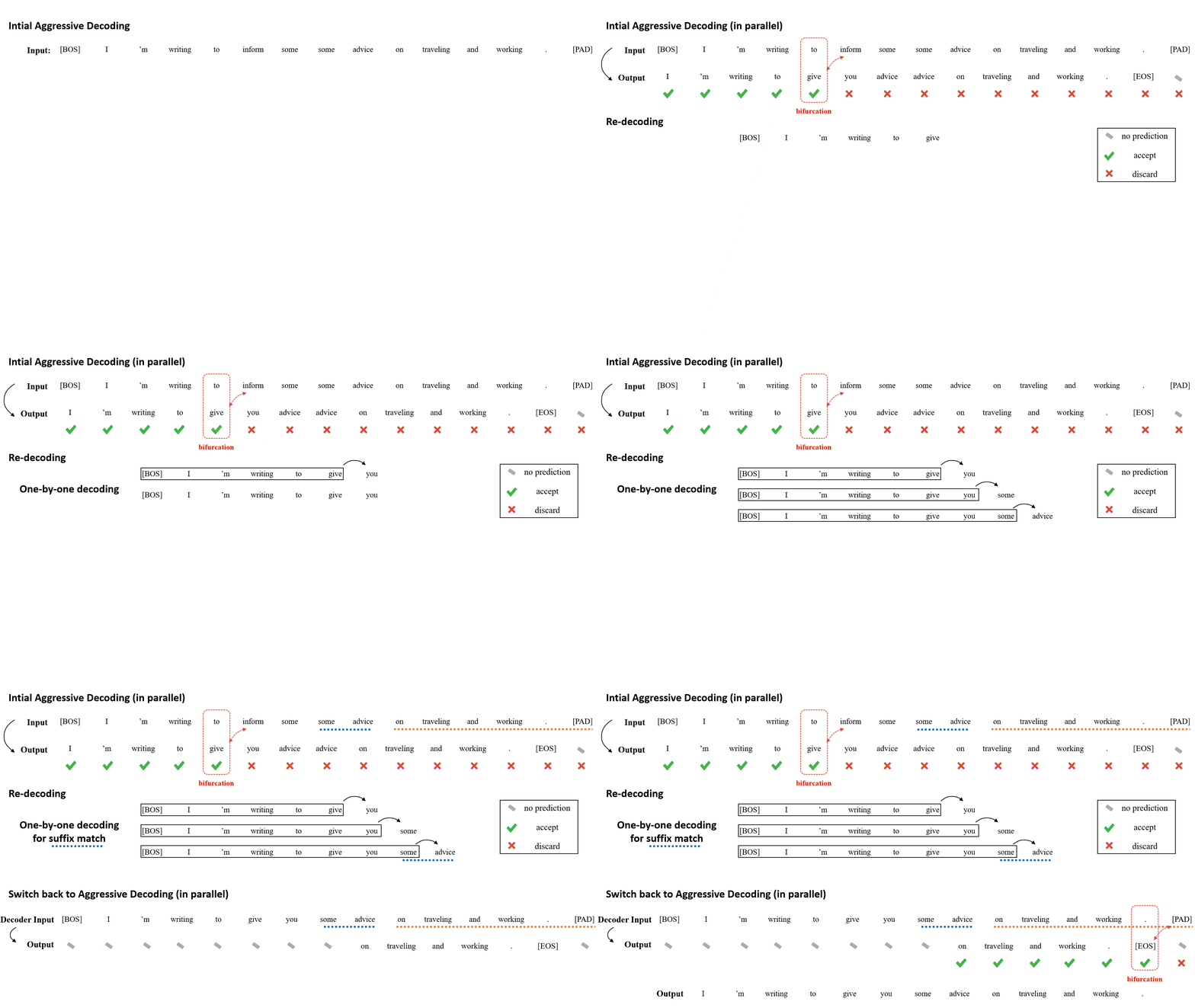
A gif demonstration of the lossless speedup mechanism of Aggressive Decoding. Aggressive Decoding speculatively uses the input text as the draft output to efficiently verify the draft results in parallel, making it possible to achieve the same result with much less time cost.

The figure above shows how Aggressive Decoding works. If we find a bifurcation during Aggressive Decoding, we discard all the predictions after the bifurcation and re-decode them using conventional one-by-one autoregressive decoding. If we find a suffix match (i.e., some advice highlighted with the blue dotted lines) between the output and the input during one-by-one re-decoding, we switch back to Aggressive Decoding by copying the tokens (highlighted with the orange dashed lines) and following the matched tokens in the input to the decoder input by assuming they will be the same. In this way, Aggressive Decoding can guarantee that the generated tokens are identical to autoregressive greedy decoding but with much fewer decoding steps, significantly improving the decoding efficiency.

Offline evaluations

We test Aggressive Decoding in grammar correction and other text rewriting tasks, such as text simplification, with a 6+6 standard transformer as well as a transformer with deep encoder and shallow decoder. All results confirm that Aggressive Decoding can introduce a significant speedup without quality loss.

    CoNLL14 NLCC-18 Wikilarge
F0.5 speedup F0.5 speedup SARI BLEU speedup
6+6 Transformer (beam=1) 61.3 1 29.4 1 36.1 90.7 1
6+6 Transformer (AD) 61.3 6.8 29.4 7.7 36.1 90.7 8
    CoNLL14
F0.5 speedup
12+2 Transformer (beam=1) 66.4 1
12+2 Transformer (AD) 66.4 4.2

And it can work even better on more powerful computing devices that excel at parallel computing (e.g., A100):
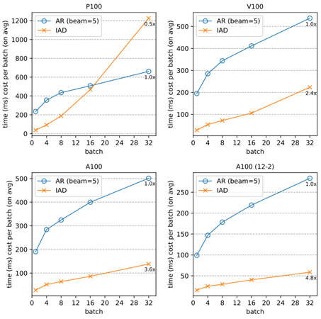
Four charts showing the speedup introduced by Aggressive Decoding in different computing devices. Aggressive Decoding can result in better speedup results in more advanced computing devices (I.e., V100 and A100 with fp16), demonstrating its huge potential in the future with even more powerful computing devices (e.g., H100 with fp8).

Online evaluation

We ran an A/B experiment between a Marian server model and an equal size server model with Aggressive Decoding using ONNX Runtime. The latter shows 2x+ improvement @p50 and 3x+ improvement @p95 and @p99 over the Marian runtime, with conventional autoregressive decoding in CPU as shown in the graph below. Moreover, it offers better efficiency stability than the previous autoregressive decoding, which varies drastically in latency (approximately proportional to the sentence length), as Aggressive Decoding substantially reduces the decoding cost with only a few steps of parallel computing regardless of the sentence length. This substantial inference time speedup resulted in a two-thirds COGS reduction in the production endpoints.

Three bar charts showing model latency comparison between the Marian server model and the ONNX server model with aggressive decoding at 50th percentile, 95th percentile and 99th percentile across fifteen regions. The first bar chart shows 2x latency improvement from the ONNX model at 50th percentile. The second and third bar charts show 3x latency improvement from the ONNX model at 95th percentile and 99th percentile.

Both offline/online evaluations confirm that Aggressive Decoding allows us to achieve significant COGS reduction without any loss of model prediction quality. Based on this intuition, we generalize[4]Aggressive Decoding to more general seq2seq tasks. Its high efficiency with lossless quality makes Aggressive Decoding likely to become the de facto decoding standard for seq2seq tasks and to play a vital role in the cost reduction of seq2seq model deployment.

Accelerate Grammar Checker with ONNX Runtime

ONNX Runtime is a high-performance engine, developed by Microsoft, that runs AI models across various hardware targets. A wide range of ML-powered Microsoft products leverage ONNX Runtime for inferencing performance acceleration. To further reduce the inferencing latency, the PyTorch Grammar Checker with Aggressive Decoding was exported to ONNX format using PyTorch-ONNX exporter, then inferenced with ONNX Runtime, which enables transformer optimizations and quantitation for CPU performance acceleration as well as model size reduction. A number of techniques are enabled in this end-to-end solution to run the advanced grammar checker model efficiently.

PyTorch provides a built-in function to export the PyTorch model to ONNX format with ease. To support the unique architecture of the grammar checker model, we enabled export of complex nested control flows to ONNX in the exporter. During this effort, we also extended the official ONNX specification on sequence type and operators to represent more complex scenarios (i.e., the autoregressive search algorithm). This eliminates the need to separately export model encoder and decoder components and stitch them together later with additional sequence generation implementation for production. With sequence type and operators support in PyTorch-ONNX exporter and ONNX Runtime, we were able to export one single ONNX graph, including encoder and decoder and sequence generation, which brings in both efficient computation and simpler inference logic. Furthermore, the shape type inference component of PyTorch ONNX exporter is enhanced to produce a valid ONNX model under stricter ONNX shape type constraints.

The innovative Aggressive Decoding algorithm introduced in the grammar checker model was originally implemented in Fairseq. To make it ONNX compatible, we reimplemented this Aggressive Decoding algorithm in HuggingFace for easy exporting. When diving into the implementation, we identified certain components that are not directly supported in the ONNX standard operator set (e.g., bifurcation detector). There are two approaches for exporting unsupported operators to ONNX and running with ONNX Runtime. We can either create a graph composing several standard ONNX operators that have equivalent semantics or implement a custom operator in ONNX Runtime with more efficient implementation. ONNX Runtime custom operator capability allows users to implement their own operators to run within ONNX Runtime with more flexibility. This is a tradeoff between implementation cost and performance. Considering the complexity of these components, the composition of standard ONNX operators might become a performance bottleneck. Hence, we introduced custom operators in ONNX Runtime to represent these components.

ONNX Runtime enables transformer optimizations and quantization, showing very promising performance gain on both CPU and GPU. We further enhanced encoder attention fusion and decoder reshape fusion for the grammar checker model. Another big challenge of supporting this model is multiple model subgraphs. We implemented subgraphs fusion in ONNX Runtime transformers optimizer and quantization tool. ONNX Runtime Quantization was applied to the whole model, further improving throughput and latency.

Quality Enhancement by GPT-3.5 LLMs

To further improve the precision and recall of the models in production, we employ the powerful GPT-3.5 as the teacher model. Specifically, the GPT-3.5 model works in the following two ways to help improve the result:

  • Training data augmentation: We fine-tune the GPT-3.5 model and use it to generate labels for massive unannotated texts. The annotations obtained are verified to be of high quality and can be used as augmented training data to enhance the performance of our model.
  • Training data cleaning: We leverage the powerful zero/few-shot capability of GPT-3.5 to distinguish between high-quality and low-quality training examples. The annotations of the identified low-quality examples are then regenerated by the GPT-3.5 model, resulting in a cleaner and higher-quality training set, which directly enhances the performance of our model.

EdgeFormer: Cost-effective parameterization for on-device seq2seq modeling

In recent years, the computational power of client devices has greatly increased, allowing for the use of deep neural networks to achieve the ultimate zero-COGS goal. However, running generative language models on these devices still poses a significant challenge, as the memory efficiency of these models must be strictly controlled. The traditional methods of compression used for neural networks in natural language understanding are often not applicable when it comes to generative language models.
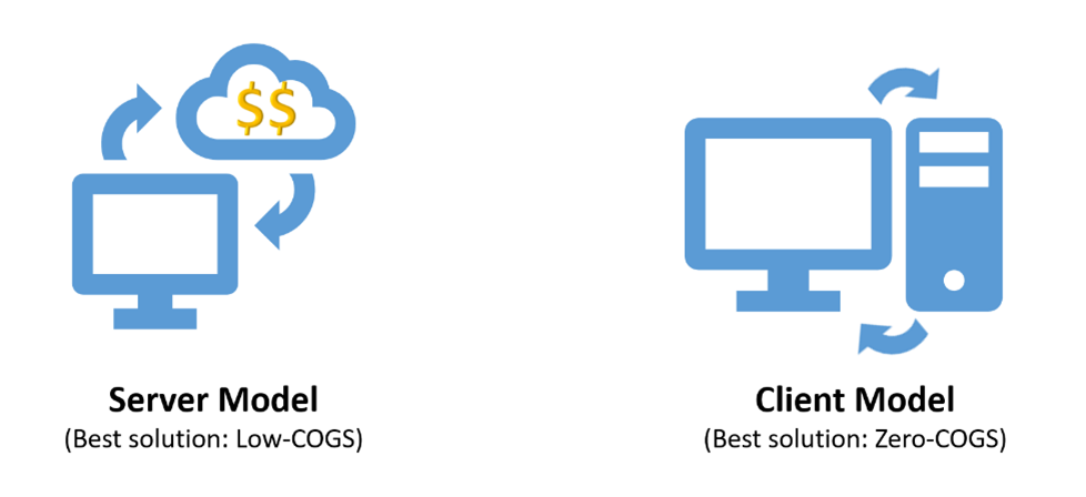
Two illustrations to show the differences between a server model and a client model.

To ship a client grammar model, the model should be highly efficient (e.g., within 100ms latency), which has already been solved by Aggressive Decoding, mentioned earlier. Moreover, the client model must be memory-efficient (e.g., within a 50MB RAM footprint), which is the main bottleneck for a powerful (generative) transformer model (usually over 50 million parameters) to run on a client device.

To address this challenge, we introduce EdgeFormer[6], a cutting-edge on-device seq2seq modeling technology for obtaining lightweight generative language models with competitive performance that can be easily run on a user’s computer.
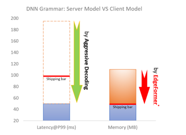
A figure shows the latency and memory shipping bar for the client DNN grammar checker. Aggressive Decoding can effectively address the latency challenge, while the memory challenge is resolved by another innovation called EdgeFormer.

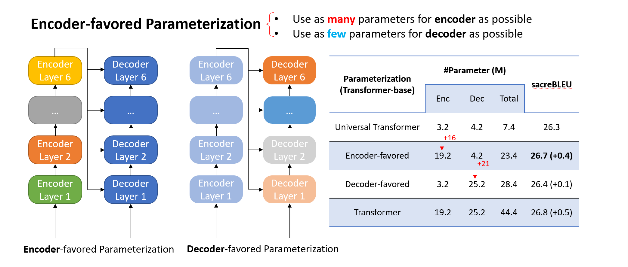
The main idea of EdgeFormer is two principles, which we proposed for cost-effective parameterization:

  • Encoder-favored parameterization
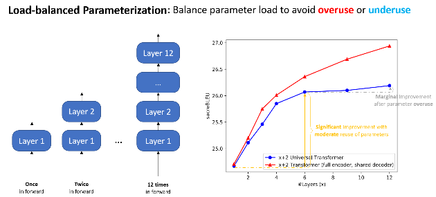
  • Load-balanced parameterization
An illustration and a table that show encoder-favored parameterization is cost-effective.
The (left) figure shows parameters’ load in different network architectures. The (right) chart shows that either underusing or overusing a parameter is undesirable, suggesting we balance the load of parameters.

We designed EdgeFormer with the above principles of cost-effective parameterization, allowing each parameter to be utilized to its maximum potential, which achieves competitive results despite the stringent computational and memory constraints of client devices.

Based on EdgeFormer, we further propose EdgeLM – the pretrained version of EdgeFormer, which is the first publicly available pretrained on-device seq2seq model that can be easily fine-tuned for seq2seq tasks with strong results. EdgeLM serves as the foundation model of the grammar client model to realize the zero-COGS goal, which achieves over 5x model size compression with minimal quality loss compared to the server model.

Inference cost reduction to empower client-device deployment

Model deployment on client devices has strict requirements on hardware usage, such as memory and disk size, to avoid interference with other user applications. ONNX Runtime shows advantages for on-device deployment along with its lightweight engine and comprehensive client-inference focused solutions, such as ONNX Runtime quantization and ONNX Runtime extensions. In addition, to maintain service quality while meeting shipping requirements, MSR introduced a series of optimization techniques, including system-aware model optimization, model metadata simplification, and deferred parameter loading as well as customized quantization strategy. Based on the EdgeFormer modeling, these system optimizations can further reduce the memory cost by 2.7x, without sacrificing model performance.

We will elaborate on each one in the following sections: 

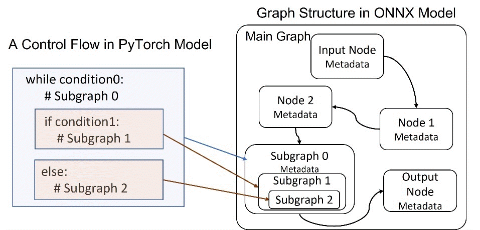
System-aware model optimization. As the model is represented as a dataflow graph, the major memory cost for this model is from the many subgraphs generated. As shown in the figure below, a branch in the PyTorch code is mapped as a subgraph. Therefore, we optimize the model implementation to reduce the usage of branch instructions. Particularly, we leverage greedy search as the decoder search algorithm, as beam search contains more branch instructions. The usage of this method can reduce memory cost by 38%

Two charts show the mapping of a PyTorch model and ONNX model graph. The left chart shows a while loop with the if_else statement as the loop body. It is an example of a control flow in a PyTorch DNN model. Each branch of the control flow is mapped to a subgraph in the right chart. The right chart illustrates an ONNX dataflow graph composed of connected nodes. Each node contains metadata. Each subgraph in the main graph is mapped to a PyTorch branch.
Mapping of PyTorch model and ONNX model graph

Model metadata simplification. Also shown in the figure above, the model contains a lot of metadata that consumes memory, such as the node name and type, input and output, and parameters. To reduce the cost, we simplify the metadata to keep only the basic required information for inference. For example, the node name is simplified from a long string to an index. Besides that, we optimize the model graph implementation in ONNX Runtime to keep just one copy of the metadata, rather than duplicating all the available metadata each time a subgraph is generated.

Deferred weight loading in ONNX Runtime. Current model files include both the model graphs and weights, which are then loaded into memory together during model initialization. However, this increases memory usage as shown in the figure below, because the weights will be copied repeatedly during model graph parsing and conversion. To avoid this, we save model graphs and weights separately. During initialization in ONNX Runtime, only the graphs are loaded into memory for actual parsing and conversion. The weights, on the other hand, still reside on disk with only the pointer kept in memory, through file mapping. The actual weight loading to memory will be deferred until the model inference. This technique can reduce the peak memory cost by 50%.
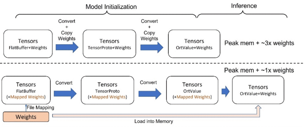
Two charts show the difference between the deferred weights loading and the default ONNX runtime implementation. The upper chart shows, in the model initialization stage, each step of model graph parsing and conversion requires a weight copy. The three steps from left to right are FlatBuffer, TensorProto, and OrtValue. During inference stage, the peak memory cost is added with three times of mode weight size. The lower chart also shows the three steps, but with mapped weights in each step. The weights are loaded until inference starts. The peak memory is thus added with the weight size only.
Deferred weights loading by file mapping during model initialization

ONNX Runtime quantization and ONNX Runtime extensions. Quantization is a well-known model compression technique that brings in both performance acceleration and model size reduction while sacrificing model accuracy. ONNX Runtime Quantization offers diverse tuning knobs to allow us to apply customized quantization strategy. Specifically, we customize the strategy as post-training, dynamic, UINT8, per-channel and all-operator quantization, for this model for minimum accuracy impact. Onnxruntime-extensions provides a set of ONNX Runtime custom operators to support the common pre- and post-processing operators for vision, text, and natural language processing models. With it, the pre- and post-processing for this model, including tokenization, string manipulation, and so on, can be integrated into one self-contained ONNX model file, leading to improved performance, simplified deployment, reduced memory usage, and better portability.

Conclusion

In this blog post, we have presented how we leveraged the cutting-edge research innovations from MSR and ONNX Runtime to optimize the server grammar checker model and achieve the ultimate zero-COGS goal with the client grammar checker model. The server model has achieved ~200% increase in inference speed while saving two-thirds of the cost, with no loss of model prediction quality. The client model has achieved over 5x model size compression with minimal quality loss compared to the server model. These optimizations have enabled us to scale quickly to more web and desktop endpoints and provide AI-powered writing assistance to millions of users around the world.

The innovation shared in this blog post is just the first milestone in our long-term continuous effort of COGS reduction for generative AI models. Our proposed approach is not limited to accelerating the neural grammar checker; it can be easily generalized and applied more broadly to scenarios such as abstractive summarization, translation, or search engines to accelerate large language models for COGS reduction[5,8], which is critical not only for Microsoft but also for the entire industry in the artificial general intelligence (AGI) era.

Reference

[1] Tao Ge, Furu Wei, Ming Zhou: Fluency Boost Learning and Inference for Neural Grammatical Error Correction. In ACL 2018.

[2] Tao Ge, Furu Wei, Ming Zhou: Reaching Human-level Performance in Automatic Grammatical Error Correction: An Empirical Study. https://arxiv.org/abs/1807.01270

[3] Xin Sun, Tao Ge, Shuming Ma, Jingjing Li, Furu Wei, Houfeng Wang: A Unified Strategy for Multilingual Grammatical Error Correction with Pre-trained Cross-lingual Language Model. In IJCAI 2022.

[4] Xin Sun, Tao Ge, Furu Wei, Houfeng Wang: Instantaneous Grammatical Error Correction with Shallow Aggressive Decoding. In ACL 2021.

[5] Tao Ge, Heming Xia, Xin Sun, Si-Qing Chen, Furu Wei: Lossless Acceleration for Seq2seq Generation with Aggressive Decoding. https://arxiv.org/pdf/2205.10350.pdf

[6] Tao Ge, Si-Qing Chen, Furu Wei: EdgeFormer: A Parameter-efficient Transformer for On-device Seq2seq Generation. In EMNLP 2022.

[7] Heidorn, George. “Intelligent Writing Assistance.” Handbook of Natural Language Processing. Robert Dale, Hermann L. Moisl, and H. L. Somers, editors. New York: Marcel Dekker, 2000: 181-207.

[8] Nan Yang, Tao Ge, Liang Wang, Binxing Jiao, Daxin Jiang, Linjun Yang, Rangan Majumder, Furu Wei: Inference with Reference: Lossless Acceleration of Large Language Models. https://arxiv.org/abs/2304.04487

The post Achieving Zero-COGS with Microsoft Editor Neural Grammar Checker appeared first on Microsoft Research.

Read More

NVIDIA Cambridge-1 AI Supercomputer Expands Reach to Researchers via the Cloud

NVIDIA Cambridge-1 AI Supercomputer Expands Reach to Researchers via the Cloud

Scientific researchers need massive computational resources that can support exploration wherever it happens. Whether they’re conducting groundbreaking pharmaceutical research, exploring alternative  energy sources or discovering new ways to prevent financial fraud, accessible state-of-the-art AI computing resources are key to driving innovation. This new model of computing can solve the challenges of generative AI and power the next wave of innovation.

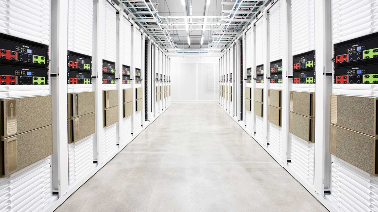
Cambridge-1, a supercomputer NVIDIA launched in the U.K. during the pandemic, has powered discoveries from some of the country’s top healthcare researchers. The system is now becoming part of NVIDIA DGX Cloud to accelerate the pace of scientific innovation and discovery — across almost every industry.

As a cloud-based resource, it will broaden access to AI supercomputing for researchers in climate science, autonomous machines, worker safety and other areas, delivered with the simplicity and speed of the cloud, ideally located for the U.K. and European access.

DGX Cloud is a multinode AI training service that makes it possible for any enterprise to access leading-edge supercomputing resources from a browser. The original Cambridge-1 infrastructure included 80 NVIDIA DGX systems; now it will join with DGX Cloud, to allow customers access to world-class infrastructure.

History of Healthcare Insights

Academia, startups and the UK’s large pharma ecosystem used the Cambridge-1 supercomputing resource to accelerate research and design new approaches to drug discovery, genomics and medical imaging with generative AI in some of the following ways:

  • InstaDeep, in collaboration with NVIDIA and the Technical University of Munich Lab, developed a 2.5 billion-parameter LLM for genomics on Cambridge-1. This project aimed to create a more accurate model for predicting the properties of DNA sequences.
  • King’s College London used Cambridge-1 to create 100,000 synthetic brain images — and made them available for free to healthcare researchers. Using the open-source AI imaging platform MONAI, the researchers at King’s created realistic, high-resolution 3D images of human brains, training in weeks versus months.
  • Oxford Nanopore used Cambridge-1 to quickly develop highly accurate, efficient models for base calling in DNA sequencing. The company also used the supercomputer to support inference for the ORG.one project, which aims to enable DNA sequencing of critically endangered species
  • Peptone, in collaboration with a pharma partner, used Cambridge-1 to run physics-based simulations to evaluate the effect of mutations on protein dynamics with the goal of better understanding why specific antibodies work efficiently. This research could improve antibody development and biologics discovery.
  • Relation Therapeutics developed a large language model which reads DNA to better understand genes, which is a key step to creating new medicines. Their research takes us a step closer to understanding how genes are controlled in certain diseases.

Read More

Beyond Fast: GeForce RTX 4060 GPU Family Gives Creators More Options to Accelerate Workflows, Starting at $299

Beyond Fast: GeForce RTX 4060 GPU Family Gives Creators More Options to Accelerate Workflows, Starting at $299

Editor’s note: This post is part of our weekly In the NVIDIA Studio series, which celebrates featured artists, offers creative tips and tricks, and demonstrates how NVIDIA Studio technology improves creative workflows. We’re also deep diving on new GeForce RTX 40 Series GPU features, technologies and resources, and how they dramatically accelerate content creation.

The GeForce RTX 4060 family will be available starting next week, bringing massive creator benefits to the popular 60-class GPUs.

The latest GPUs in the 40 Series come backed by NVIDIA Studio technologies, including hardware acceleration for 3D, video and AI workflows; optimizations for RTX hardware in over 110 of the most popular creative apps; and exclusive Studio apps like Omniverse, Broadcast and Canvas.

Real-time ray-tracing renderer D5 Render introduced support for NVIDIA DLSS 3 technology, enabling super smooth real-time rendering experiences, so creators can work with larger scenes without sacrificing speed or interactivity.

Plus, the new Into the Omniverse series highlights the latest advancements to NVIDIA Omniverse, a platform furthering the evolution of the metaverse with the OpenUSD framework. The series showcases how artists, developers and enterprises can use the open development platform to transform their 3D workflows. The first installment highlights an update coming soon to the Adobe Substance 3D Painter Connector.

In addition, NVIDIA 3D artist Daniel Barnes returns this week In the NVIDIA Studio to share his mesmerizing, whimsical animation, Wormhole 00527.

Beyond Fast

The GeForce RTX 4060 family is powered by the ultra-efficient NVIDIA Ada Lovelace architecture with fourth-generation Tensor Cores for AI content creation, third-generation RT Cores and compatibility with DLSS 3 for ultra-fast 3D rendering, as well as the eighth-generation NVIDIA encoder (NVENC), now with support for AV1.

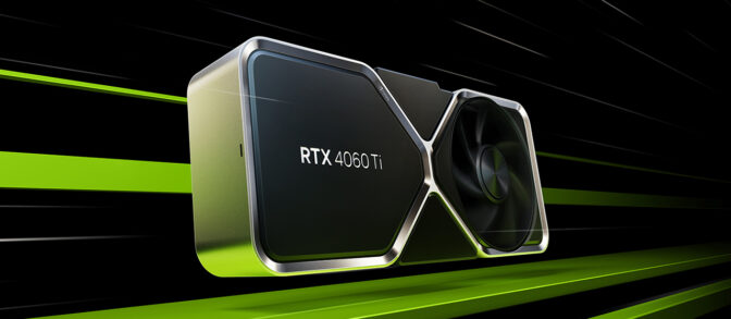
The GeForce RTX 4060 Ti GPU.

3D modelers can build and edit realistic 3D models in real time, up to 45% faster than the previous generation, thanks to third-generation RT Cores, DLSS 3 and the NVIDIA Omniverse platform.

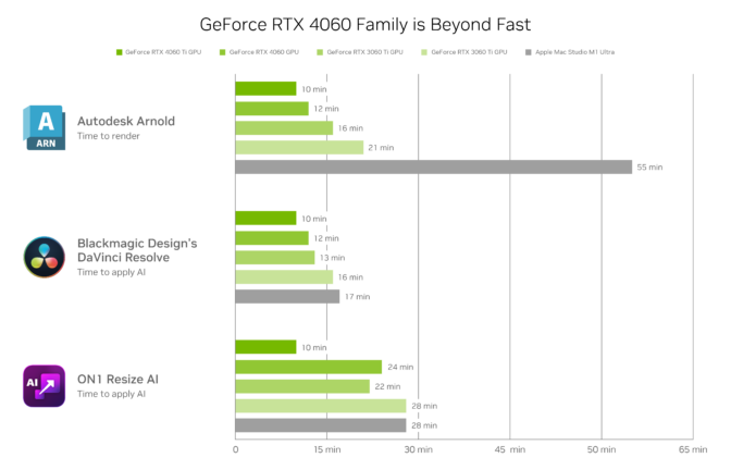
Tested on GeForce RTX 4060 and 3060 GPUs. Maya with Arnold 2022 (7.1.1) measures render time of NVIDIA SOL 3D model. DaVinci Resolve measures FPS applying Magic Mask effect “Faster” quality setting to 4K resolution. ON1 Resize AI measures time required to apply effect to batch of 10 photos. Time measurement is normalized for easier comparison across tests.

Video editors specializing in Adobe Premiere Pro, Blackmagic Design’s DaVinci Resolve and more have at their disposal a variety of AI-powered effects, such as auto-reframe, magic mask and depth estimation. Fourth-generation Tensor Cores seamlessly hyper-accelerate these effects, so creators can stay in their flow states.

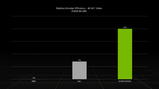
Broadcasters can jump into next-generation livestreaming with the eighth-generation NVENC with support for AV1. The new encoder is 40% more efficient, making livestreams appear as if there were a 40% increase in bitrate — a big boost in image quality that enables 4K streaming on apps like OBS Studio and platforms such as YouTube and Discord.

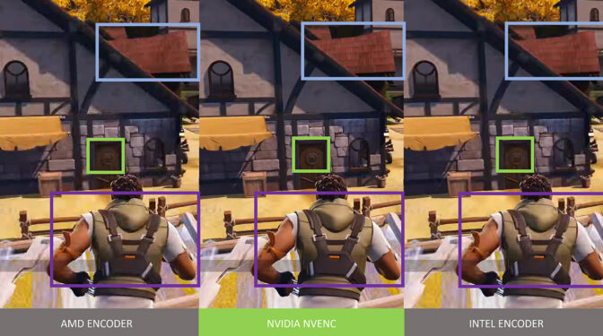
10 Mbps with default OBS streaming settings.

NVENC boasts the most efficient hardware encoding available, providing significantly better quality than other GPUs. At the same bitrate, images will look better, sharper and have less artifacts, like in the example above.

Encode quality comparison, measured with BD-BR.

Creators are embracing AI en masse. DLSS 3 multiplies frame rates in popular 3D apps. ON1 ResizeAI, software that enables high-quality photo enlargement, is sped up 24% compared with last-generation hardware. DaVinci Resolve’s AI Magic Mask feature saves video editors considerable time automating the highly manual process of rotoscoping, carried out 20% faster than the previous generation.

The GeForce RTX 4060 Ti (8GB) will be available starting Wednesday, May 24, at $399. The GeForce RTX 4060 Ti (16GB) will be available in July, starting at $499. GeForce RTX 4060 will also be available in July, starting at $299.

Visit the Studio Shop for GeForce RTX 4060-powered NVIDIA Studio systems when available, and explore the range of high-performance Studio products.

D5 Render, DLSS 3 Combine to Beautiful Effect

D5 Render adds support for NVIDIA DLSS 3, bringing a vastly improved real-time experience to architects, designers, interior designers and 3D artists.

Such professionals want to navigate scenes smoothly while editing, and demonstrate their creations to clients in the highest quality. Scenes can be incredibly detailed and complex, making it difficult to maintain high real-time viewport frame rates and present in original quality.

D5 is coveted by many artists for its global illumination technology, called D5 GI, which delivers high-quality lighting and shading effects in real time, without sacrificing workflow efficiency.

D5 Render and DLSS 3 work brilliantly to create photorealistic imagery.

By integrating DLSS 3, which combines AI-powered DLSS Frame Generation and Super Resolution technologies, real-time viewport frame rates increase up to 3x, making creator experiences buttery smooth. This allows designers to deal with larger scenes, higher-quality models and textures — all in real time — while maintaining a smooth, interactive viewport.

Learn more about the update.

Venture ‘Into the Omniverse’

NVIDIA Omniverse is a key component of the NVIDIA Studio platform and the future of collaborative 3D content creation.

A new monthly blog series, Into the Omniverse, showcases how artists, developers and enterprises can transform their creative workflows using the latest Omniverse advancements.

This month, 3D creators across industries are set to benefit from the pairing of Omniverse and the Adobe Substance 3D suite of creative tools.

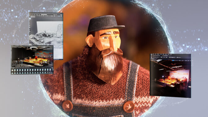
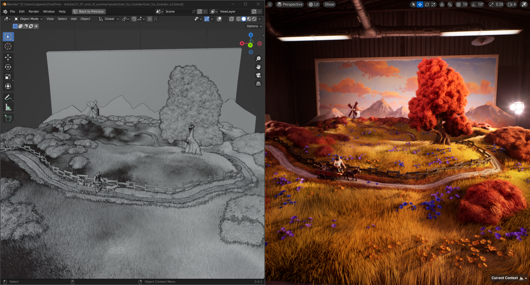
“End of Summer,” created by the Adobe Substance 3D art and development team, built in Omniverse.

An upcoming update to the Omniverse Connector for Adobe Substance 3D Painter will dramatically increase flexibility for users, with new capabilities including an export feature using Universal Scene Description (OpenUSD), an open, extensible file framework enabling non-destructive workflows and collaboration in scene creation.

Find details in the blog and check in every month for more Omniverse news.

Your Last Worm-ing

NVIDIA 3D artist Daniel Barnes has a simple initial approach to his work: sketch until something seems cool enough to act on. While his piece Wormhole 00527 was no exception to this usual process, an emotional component made a significant impact on it.


“After the pandemic and various global events, I took even more interest in spaceships and escape pods,” said Barnes. “It was just an abstract form of escapism that really played on the idea of ‘get me out of here,’ which I think we all experienced at one point, being inside so much.”

Barnes imagined Wormhole 00527 to comprise each blur one might pass by as an alternate star system — a place on the other side of the galaxy where things are really similar but more peaceful, he said. “An alternate Earth of sorts,” the artist added.

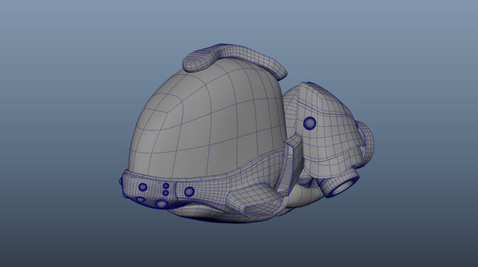
Sculpting on his tablet one night in the Nomad app, Barnes imported a primitive model into Autodesk Maya for further refinement. He retopologized the scene, converting high-resolution models into much smaller files that can be used for animation.

Modeling in Autodesk Maya.

“I’ve been creating in 3D for over a decade now, and GeForce RTX graphics cards have been able to power multiple displays smoothly and run my 3D software viewports at great speeds. Plus, rendering in real time on some projects is great for fast development.” — Daniel Barnes

Barnes then took a screenshot, further sketched out his modeling edits and made lighting decisions in Adobe Photoshop.

His GeForce RTX 4090 GPU gives him access to over 30 GPU-accelerated features for quickly, smoothly modifying and adjusting images. These features include blur gallery, object selection and perspective warp.

Back in Autodesk Maya, Barnes used the quad-draw tool — a streamlined, one-tool workflow for retopologizing meshes — to create geometry, adding break-in panels that would be advantageous for animating.

So this is what a wormhole looks like.

Barnes used Chaos V-Ray with Autodesk Maya’s Z-depth feature, which provides information about each object’s distance from the camera in its current view. Each pixel representing the object is evaluated for distance individually — meaning different pixels for the same object can have varying grayscale values. This made it far easier for Barnes to tweak depth of field and add motion-blur effects.

Example of Z-depth. Image courtesy of Chaos V-Ray with Autodesk Maya.

He also added a combination of lights and applied materials with ease. Deploying RTX-accelerated ray tracing and AI denoising with the default Autodesk Arnold renderer enabled smooth movement in the viewport, resulting in beautifully photorealistic renders.

The Z-depth feature made it easier to apply motion-blur effects.

He finished the project by compositing in Adobe After Effects, using GPU-accelerated features for faster rendering with NVIDIA CUDA technology.

3D artist Daniel Barnes.

When asked what his favorite creative tools are, Barnes didn’t hesitate. “Definitely my RTX cards and nice large displays!” he said.

Check out Barnes’ portfolio on Instagram.

Follow NVIDIA Studio on Instagram, Twitter and Facebook. Access tutorials on the Studio YouTube channel and get updates directly in your inbox by subscribing to the Studio newsletter. 

Get started with NVIDIA Omniverse by downloading the standard license free, or learn how Omniverse Enterprise can connect your team. Developers can get started with Omniverse resources. Stay up to date on the platform by subscribing to the newsletter, and follow NVIDIA Omniverse on Instagram, Medium and Twitter

For more, join the Omniverse community and check out the Omniverse forums, Discord server, Twitch and YouTube channels.

Read More

First Xbox Title Joins GeForce NOW

First Xbox Title Joins GeForce NOW

Get ready for action — the first Xbox game title is now streaming from GeForce GPUs in the cloud directly to GeForce NOW members, with more to come later this month.

Gears 5 comes to the service this GFN Thursday. Keep reading to find out what other entries from the Xbox library will be streaming on GeForce NOW soon.

Also, time’s almost up on an exclusive discount for six-month GeForce NOW Priority memberships. Sign up today to save 40% before the offer ends on Sunday, May 21.

All Geared Up

Gears 5 on GeForce NOW
The gang’s all here.

NVIDIA and Microsoft have been working together to bring the first Xbox PC titles to the GeForce NOW library. With their gaming fueled by GeForce GPU servers in the cloud, members can access the best of Xbox Game Studios and Bethesda titles across nearly any device, including underpowered PCs, Macs, iOS and Android mobile devices, NVIDIA SHIELD TV, supported smart TVs and more.

Gears 5 from The Coalition is the first PC title from Xbox Game Studios to hit GeForce NOW. The latest entry in the Gears saga includes an acclaimed campaign playable solo or cooperatively, plus a variety of PvE and PvP modes to team up and battle in.

More Microsoft titles will follow shortly, starting with Deathloop, Grounded and Pentiment on Thursday, May 25.

Members will be able to stream these Xbox PC hits purchased through Steam on PCs, macOS devices, Chromebooks, smartphones and other devices. Support for Microsoft Store will become available in the coming months. Learn more about Xbox PC game support on GeForce NOW.

GeForce NOW Priority members can skip the wait and play Gears 5 or one of the other 1,600+ supported titles at 1080p 60 frames per second. Or go Ultimate for an upgraded experience, playing at up to 4K 120 fps for gorgeous graphics, or up to 240 fps for ultra-low latency that gives the competitive edge.

Microsoft on GeForce NOW
Like peanut butter and jelly.

GeForce NOW members will see more PC games from Xbox added regularly and can keep up with the latest news and release dates through GFN Thursday updates.

Green Light Special

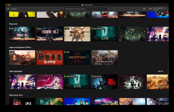
The latest GeForce NOW app updates are rolling out now. Version 2.0.52 brings a few fit-and-finish updates for members, including a new way to easily catch game discounts, content and more.

Wall of Games GeForce NOW
Look for the latest deals, downloadable content and more in the latest GeForce NOW app update.

Promotional tags can be found on featured games throughout the app on PC and macOS. The tags are curated to highlight the most compelling offers available on the 1,600+ GeForce NOW-supported games. Keep an eye out for these promotional tags, which showcase new downloadable content, discounts, free games and more.

The update also includes in-app search improvements, surround-sound support in the browser experience on Windows and macOS, updated in-game button prompts for members using DualShock 4 and DualSense controllers, and more. Check out the in-app release highlights for more info.

Play for Today

Outlast Trials on GeForce NOW
They say things aren’t so scary when you’re with friends. ‘The Outlast Trials’ aims to prove them wrong.

Don’t get spooked in The Outlast Trials, newly supported this week on GeForce NOW. Go it alone or team up in this multiplayer edition of the survival horror franchise. Avoid the monstrosities waiting in the Murkoff experiments while using new tools to aid stealth, create opportunities to flee, slow enemies and more.

With support for more games every week, there’s always a new adventure around the corner. Here’s this week’s additions:

  • Tin Hearts (New release on Steam, May 16)
  • The Outlast Trials (New release on Steam, May 18)
  • Gears 5 (Steam)

With the weekend kicking off, what are you gearing up to play? Let us know on Twitter or in the comments below.

Read More

Build a serverless meeting summarization backend with large language models on Amazon SageMaker JumpStart

Build a serverless meeting summarization backend with large language models on Amazon SageMaker JumpStart

AWS delivers services that meet customers’ artificial intelligence (AI) and machine learning (ML) needs with services ranging from custom hardware like AWS Trainium and AWS Inferentia to generative AI foundation models (FMs) on Amazon Bedrock. In February 2022, AWS and Hugging Face announced a collaboration to make generative AI more accessible and cost efficient.

Generative AI has grown at an accelerating rate from the largest pre-trained model in 2019 having 330 million parameters to more than 500 billion parameters today. The performance and quality of the models also improved drastically with the number of parameters. These models span tasks like text-to-text, text-to-image, text-to-embedding, and more. You can use large language models (LLMs), more specifically, for tasks including summarization, metadata extraction, and question answering.

Amazon SageMaker JumpStart is an ML hub that can helps you accelerate your ML journey. With JumpStart, you can access pre-trained models and foundation models from the Foundations Model Hub to perform tasks like article summarization and image generation. Pre-trained models are fully customizable for your use cases and can be easily deployed into production with the user interface or SDK. Most importantly, none of your data is used to train the underlying models. Because all data is encrypted and doesn’t leave the virtual private cloud (VPC), you can trust that your data will remain private and confidential.

This post focuses on building a serverless meeting summarization using Amazon Transcribe to transcribe meeting audio and the Flan-T5-XL model from Hugging Face (available on JumpStart) for summarization.

Solution overview

The Meeting Notes Generator Solution creates an automated serverless pipeline using AWS Lambda for transcribing and summarizing audio and video recordings of meetings. The solution can be deployed with other FMs available on JumpStart.

The solution includes the following components:

  • A shell script for creating a custom Lambda layer
  • A configurable AWS CloudFormation template for deploying the solution
  • Lambda function code for starting Amazon Transcribe transcription jobs
  • Lambda function code for invoking a SageMaker real-time endpoint hosting the Flan T5 XL model

The following diagram illustrates this architecture.

Architecture Diagram

As shown in the architecture diagram, the meeting recordings, transcripts, and notes are stored in respective Amazon Simple Storage Service (Amazon S3) buckets. The solution takes an event-driven approach to transcribe and summarize upon S3 upload events. The events trigger Lambda functions to make API calls to Amazon Transcribe and invoke the real-time endpoint hosting the Flan T5 XL model.

The CloudFormation template and instructions for deploying the solution can be found in the GitHub repository.

Real-time inference with SageMaker

Real-time inference on SageMaker is designed for workloads with low latency requirements. SageMaker endpoints are fully managed and support multiple hosting options and auto scaling. Once created, the endpoint can be invoked with the InvokeEndpoint API. The provided CloudFormation template creates a real-time endpoint with the default instance count of 1, but it can be adjusted based on expected load on the endpoint and as the service quota for the instance type permits. You can request service quota increases on the Service Quotas page of the AWS Management Console.

The following snippet of the CloudFormation template defines the SageMaker model, endpoint configuration, and endpoint using the ModelData and ImageURI of the Flan T5 XL from JumpStart. You can explore more FMs on Getting started with Amazon SageMaker JumpStart. To deploy the solution with a different model, replace the ModelData and ImageURI parameters in the CloudFormation template with the desired model S3 artifact and container image URI, respectively. Check out the sample notebook on GitHub for sample code on how to retrieve the latest JumpStart model artifact on Amazon S3 and the corresponding public container image provided by SageMaker.

  # SageMaker Model
  SageMakerModel:
    Type: AWS::SageMaker::Model
    Properties:
      ModelName: !Sub ${AWS::StackName}-SageMakerModel
      Containers:
        - Image: !Ref ImageURI
          ModelDataUrl: !Ref ModelData
          Mode: SingleModel
          Environment: {
            "MODEL_CACHE_ROOT": "/opt/ml/model",
            "SAGEMAKER_ENV": "1",
            "SAGEMAKER_MODEL_SERVER_TIMEOUT": "3600",
            "SAGEMAKER_MODEL_SERVER_WORKERS": "1",
            "SAGEMAKER_PROGRAM": "inference.py",
            "SAGEMAKER_SUBMIT_DIRECTORY": "/opt/ml/model/code/",
            "TS_DEFAULT_WORKERS_PER_MODEL": 1
          }
      EnableNetworkIsolation: true
      ExecutionRoleArn: !GetAtt SageMakerExecutionRole.Arn

  # SageMaker Endpoint Config
  SageMakerEndpointConfig:
    Type: AWS::SageMaker::EndpointConfig
    Properties:
      EndpointConfigName: !Sub ${AWS::StackName}-SageMakerEndpointConfig
      ProductionVariants:
        - ModelName: !GetAtt SageMakerModel.ModelName
          VariantName: !Sub ${SageMakerModel.ModelName}-1
          InitialInstanceCount: !Ref InstanceCount
          InstanceType: !Ref InstanceType
          InitialVariantWeight: 1.0
          VolumeSizeInGB: 40

  # SageMaker Endpoint
  SageMakerEndpoint:
    Type: AWS::SageMaker::Endpoint
    Properties:
      EndpointName: !Sub ${AWS::StackName}-SageMakerEndpoint
      EndpointConfigName: !GetAtt SageMakerEndpointConfig.EndpointConfigName

Deploy the solution

For detailed steps on deploying the solution, follow the Deployment with CloudFormation section of the GitHub repository.

If you want to use a different instance type or more instances for the endpoint, submit a quota increase request for the desired instance type on the AWS Service Quotas Dashboard.

To use a different FM for the endpoint, replace the ImageURI and ModelData parameters in the CloudFormation template for the corresponding FM.

Test the solution

After you deploy the solution using the Lambda layer creation script and the CloudFormation template, you can test the architecture by uploading an audio or video meeting recording in any of the media formats supported by Amazon Transcribe. Complete the following steps:

  1. On the Amazon S3 console, choose Buckets in the navigation pane.
  2. From the list of S3 buckets, choose the S3 bucket created by the CloudFormation template named meeting-note-generator-demo-bucket-<aws-account-id>.
  3. Choose Create folder.
  4. For Folder name, enter the S3 prefix specified in the S3RecordingsPrefix parameter of the CloudFormation template (recordings by default).
  5. Choose Create folder.
  6. In the newly created folder, choose Upload.
  7. Choose Add files and choose the meeting recording file to upload.
  8. Choose Upload.

Now we can check for a successful transcription.

  1. On the Amazon Transcribe console, choose Transcription jobs in the navigation pane.
  2. Check that a transcription job with a corresponding name to the uploaded meeting recording has the status In progress or Complete.
  3. When the status is Complete, return to the Amazon S3 console and open the demo bucket.
  4. In the S3 bucket, open the transcripts/ folder.
  5. Download the generated text file to view the transcription.

We can also check the generated summary.

  1. In the S3 bucket, open the notes/ folder.
  2. Download the generated text file to view the generated summary.

Prompt engineering

Even though LLMs have improved in the last few years, the models can only take in finite inputs; therefore, inserting an entire transcript of a meeting may exceed the limit of the model and cause an error with the invocation. To design around this challenge, we can break down the context into manageable chunks by limiting the number of tokens in each invocation context. In this sample solution, the transcript is broken down into smaller chunks with a maximum limit on the number of tokens per chunk. Then each transcript chunk is summarized using the Flan T5 XL model. Finally, the chunk summaries are combined to form the context for the final combined summary, as shown in the following diagram.

The following code from the GenerateMeetingNotes Lambda function uses the Natural Language Toolkit (NLTK) library to tokenize the transcript, then it chunks the transcript into sections, each containing up to a certain number of tokens:

# Chunk transcript into chunks
transcript = contents['results']['transcripts'][0]['transcript']
transcript_tokens = word_tokenize(transcript)

num_chunks = int(math.ceil(len(transcript_tokens) / CHUNK_LENGTH))
transcript_chunks = []
for i in range(num_chunks):
    if i == num_chunks - 1:
        chunk = TreebankWordDetokenizer().detokenize(transcript_tokens[CHUNK_LENGTH * i:])
    else:
        chunk = TreebankWordDetokenizer().detokenize(transcript_tokens[CHUNK_LENGTH * i:CHUNK_LENGTH * (i + 1)])
    transcript_chunks.append(chunk)

After the transcript is broken up into smaller chunks, the following code invokes the SageMaker real-time inference endpoint to get summaries of each transcript chunk:

# Summarize each chunk
chunk_summaries = []
for i in range(len(transcript_chunks)):
    text_input = '{}n{}'.format(transcript_chunks[i], instruction)
    payload = {
        "text_inputs": text_input,
        "max_length": 100,
        "num_return_sequences": 1,
        "top_k": 50,
        "top_p": 0.95,
        "do_sample": True
    }
    query_response = query_endpoint_with_json_payload(json.dumps(payload).encode('utf-8'))
    generated_texts = parse_response_multiple_texts(query_response)
    chunk_summaries.append(generated_texts[0])
    print(generated_texts[0])

Finally, the following code snippet combines the chunk summaries as the context to generate a final summary:

# Create a combined summary
text_input = '{}n{}'.format(' '.join(chunk_summaries), instruction)
payload = {
    "text_inputs": text_input,
    "max_length": 100,
    "num_return_sequences": 1,
    "top_k": 50,
    "top_p": 0.95,
    "do_sample": True
}
query_response = query_endpoint_with_json_payload(json.dumps(payload).encode('utf-8'))
generated_texts = parse_response_multiple_texts(query_response)

results = {
    "summary": generated_texts,
    "chunk_summaries": chunk_summaries
}

The full GenerateMeetingNotes Lambda function can be found in the GitHub repository.

Clean up

To clean up the solution, complete the following steps:

  1. Delete all objects in the demo S3 bucket and the logs S3 bucket.
  2. Delete the CloudFormation stack.
  3. Delete the Lambda layer.

Conclusion

This post demonstrated how to use FMs on JumpStart to quickly build a serverless meeting notes generator architecture with AWS CloudFormation. Combined with AWS AI services like Amazon Transcribe and serverless technologies like Lambda, you can use FMs on JumpStart and Amazon Bedrock to build applications for various generative AI use cases.

For additional posts on ML at AWS, visit the AWS ML Blog.


About the author

Eric Kim is a Solutions Architect (SA) at Amazon Web Services. He works with game developers and publishers to build scalable games and supporting services on AWS. He primarily focuses on applications of artificial intelligence and machine learning.

Read More

Prepare training and validation dataset for facies classification using Snowflake integration and train using Amazon SageMaker Canvas

Prepare training and validation dataset for facies classification using Snowflake integration and train using Amazon SageMaker Canvas

This post is co-written with Thatcher Thornberry from bpx energy. 

Facies classification is the process of segmenting lithologic formations from geologic data at the wellbore location. During drilling, wireline logs are obtained, which have depth-dependent geologic information. Geologists are deployed to analyze this log data and determine depth ranges for potential facies of interest from the different types of log data. Accurately classifying these regions is critical for the drilling processes that follow.

Facies classification using AI and machine learning (ML) has become an increasingly popular area of investigation for many oil majors. Many data scientists and business analysts at large oil companies don’t have the necessary skillset to run advanced ML experiments on important tasks such as facies classification. To address this, we show you how to easily prepare and train a best-in-class ML classification model on this problem.

In this post, aimed primarily at those who are already using Snowflake, we explain how you can import both training and validation data for a facies classification task from Snowflake into Amazon SageMaker Canvas and subsequently train the model using a 3+ category prediction model.

Solution overview

Our solution consists of the following steps:

  1. Upload facies CSV data from your local machine to Snowflake. For this post, we use data from the following open-source GitHub repo.
  2. Configure AWS Identity and Access Management (IAM) roles for Snowflake and create a Snowflake integration.
  3. Create a secret for Snowflake credentials (optional, but advised).
  4. Import Snowflake directly into Canvas.
  5. Build a facies classification model.
  6. Analyze the model.
  7. Run batch and single predictions using the multi-class model.
  8. Share the trained model to Amazon SageMaker Studio.

Prerequisites

Prerequisites for this post include the following:

Upload facies CSV data to Snowflake

In this section, we take two open-source datasets and upload them directly from our local machine to a Snowflake database. From there, we set up an integration layer between Snowflake and Canvas.

  1. Download the training_data.csv and validation_data_nofacies.csv files to your local machine. Make note of where you saved them.
  2. Ensuring that you have the correct Snowflake credentials and have installed the Snowflake CLI desktop app, you can federate in. For more information, refer to Log into SnowSQL.
  3. Select the appropriate Snowflake warehouse to work within, which in our case is COMPUTE_WH:
USE WAREHOUSE COMPUTE_WH;

  1. Choose a database to use for the remainder of the walkthrough:
use demo_db;
  1. Create a named file format that will describe a set of staged data to access or load into Snowflake tables.

This can be run either in the Snowflake CLI or in a Snowflake worksheet on the web application. For this post, we run a SnowSQL query in the web application. See Getting Started With Worksheets for instructions to create a worksheet on the Snowflake web application.

  1. Create a table in Snowflake using the CREATE statement.

The following statement creates a new table in the current or specified schema (or replaces an existing table).

It’s important that the data types and the order in which they appear are correct, and align with what is found in the CSV files that we previously downloaded. If they’re inconsistent, we’ll run into issues later when we try to copy the data across.

  1. Do the same for the validation database.

Note that the schema is a little different to the training data. Again, ensure that the data types and column or feature orders are correct.

  1. Load the CSV data file from your local system into the Snowflake staging environment:
    • The following is the syntax of the statement for Windows OS:
      put file://D:path-to-file.csv @DB_Name.PUBLIC.%table_name;

    • The following is the syntax of the statement for Mac OS:
      put file:///path-to-file.csv @DB_NAME.PUBLIC.%table_name;

The following screenshot shows an example command and output from within the SnowSQL CLI.

  1. Copy the data into the target Snowflake table.

Here, we load the training CSV data to the target table, which we created earlier. Note that you have to do this for both the training and validation CSV files, copying them into the training and validation tables, respectively.

  1. Verify that the data has been loaded into the target table by running a SELECT query (you can do this for both the training and validation data):
select * from TRAINING_DATA

Configure Snowflake IAM roles and create the Snowflake integration

As a prerequisite for this section, please follow the official Snowflake documentation on how to configure a Snowflake Storage Integration to Access Amazon S3.

Retrieve the IAM user for your Snowflake account

Once you have successfully configured your Snowflake storage integration, run the following DESCRIBE INTEGRATION command to retrieve the ARN for the IAM user that was created automatically for your Snowflake account:

DESC INTEGRATION SAGEMAKER_CANVAS_INTEGRATION;

Record the following values from the output:

  • STORAGE_AWS_IAM_USER_ARN – The IAM user created for your Snowflake account
  • STORAGE_AWS_EXTERNAL_ID – The external ID needed to establish a trust relationship

Update the IAM role trust policy

Now we update the trust policy:

  1. On the IAM console, choose Roles in the navigation pane.
  2. Choose the role you created.
  3. On the Trust relationship tab, choose Edit trust relationship.
  4. Modify the policy document as shown in the following code with the DESC STORAGE INTEGRATION output values you recorded in the previous step.
{
    "Version": "2012-10-17",
    "Statement": [
        {
            "Sid": "",
            "Effect": "Allow",
            "Principal": {
                "AWS": "<snowflake_user_arn>"
            },
            "Action": "sts:AssumeRole",
            "Condition": {
                "StringEquals": {
                    "sts:ExternalId": "<snowflake_external_id>"
                }
            }
        }
    ]
}
  1. Choose Update trust policy.

Create an external stage in Snowflake

We use an external stage within Snowflake for loading data from an S3 bucket in your own account into Snowflake. In this step, we create an external (Amazon S3) stage that references the storage integration you created. For more information, see Creating an S3 Stage.

This requires a role that has the CREATE_STAGE privilege for the schema as well as the USAGE privilege on the storage integration. You can grant these privileges to the role as shown in the code in the next step.

Create the stage using the CREATE_STAGE command with placeholders for the external stage and S3 bucket and prefix. The stage also references a named file format object called my_csv_format:

grant create stage on schema public to role <iam_role>;
grant usage on integration SAGEMAKER_CANVAS_INTEGRATION to role <iam_role_arn>;
create stage <external_stage>
storage_integration = SAGEMAKER_CANVAS_INTEGRATION
url = '<s3_bucket>/<prefix>'
file_format = my_csv_format;

Create a secret for Snowflake credentials

Canvas allows you to use the ARN of an AWS Secrets Manager secret or a Snowflake account name, user name, and password to access Snowflake. If you intend to use the Snowflake account name, user name, and password option, skip to the next section, which covers adding the data source.

To create a Secrets Manager secret manually, complete the following steps:

  1. On the Secrets Manager console, choose Store a new secret.
  2. For Select secret type¸ select Other types of secrets.
  3. Specify the details of your secret as key-value pairs.

The names of the key are case-sensitive and must be lowercase.

If you prefer, you can use the plaintext option and enter the secret values as JSON:

{
"username": "<snowflake username>",
"password": "<snowflake password>",
"accountid": "<snowflake account id>"
}
  1. Choose Next.
  2. For Secret name, add the prefix AmazonSageMaker (for example, our secret is AmazonSageMaker-CanvasSnowflakeCreds).
  3. In the Tags section, add a tag with the key SageMaker and value true.

  1. Choose Next.
  2. The rest of the fields are optional; choose Next until you have the option to choose Store to store the secret.
  3. After you store the secret, you’re returned to the Secrets Manager console.
  4. Choose the secret you just created, then retrieve the secret ARN.
  5. Store this in your preferred text editor for use later when you create the Canvas data source.

Import Snowflake directly into Canvas

To import your facies dataset directly into Canvas, complete the following steps:

  1. On the SageMaker console, choose Amazon SageMaker Canvas in the navigation pane.
  2. Choose your user profile and choose Open Canvas.
  3. On the Canvas landing page, choose Datasets in the navigation pane.
  4. Choose Import.

  1. Click on Snowflake in the below image and then immediately “Add Connection”.
  2. Enter the ARN of the Snowflake secret that we previously created, the storage integration name (SAGEMAKER_CANVAS_INTEGRATION), and a unique connection name of your choosing.
  3. Choose Add connection.

If all the entries are valid, you should see all the databases associated with the connection in the navigation pane (see the following example for NICK_FACIES).

  1. Choose the TRAINING_DATA table, then choose Preview dataset.

If you’re happy with the data, you can edit the custom SQL in the data visualizer.

  1. Choose Edit in SQL.
  2. Run the following SQL command before importing into Canvas. (This assumes that the database is called NICK_FACIES. Replace this value with your database name.)
SELECT "FACIES", "FORMATION", "WELL_NAME", "DEPTH", "GR", "ILD_LOG10", "DELTAPHI", "PHIND", "PE", "NM_M", "RELPOS" FROM "NICK_FACIES"."PUBLIC"."TRAINING_DATA";

Something similar to the following screenshot should appear in the Import preview section.

  1. If you’re happy with the preview, choose Import data.

  1. Choose an appropriate data name, ensuring that it’s unique and fewer than 32 characters long.
  2. Use the following command to import the validation dataset, using the same method as earlier:
SELECT "FORMATION", "WELL_NAME", "DEPTH", "GR", "ILD_LOG10", "DELTAPHI", "PHIND", "PE", "NM_M", "RELPOS" FROM "NICK_FACIES"."PUBLIC"."VALIDATION_DATA";

Build a facies classification model

To build your facies classification model, complete the following steps:

  1. Choose Models in the navigation pane, then choose New Model.
  2. Give your model a suitable name.
  3. On the Select tab, choose the recently imported training dataset, then choose Select dataset.
  4. On the Build tab, drop the WELL_NAME column.

We do this because the well names themselves aren’t useful information for the ML model. They are merely arbitrary names that we find useful to distinguish between the wells themselves. The name we give a particular well is irrelevant to the ML model.

  1. Choose FACIES as the target column.
  2. Leave Model type as 3+ category prediction.
  3. Validate the data.
  4. Choose Standard build.

Your page should look similar to the following screenshot just before building your model.

After you choose Standard build, the model enters the analyze stage. You’re provided an expected build time. You can now close this window, log out of Canvas (in order to avoid charges), and return to Canvas at a later time.

Analyze the facies classification model

To analyze the model, complete the following steps:

  1. Federate back into Canvas.
  2. Locate your previously created model, choose View, then choose Analyze.
  3. On the Overview tab, you can see the impact that individual features are having on the model output.
  4. In the right pane, you can visualize the impact that a given feature (X axis) is having on the prediction of each facies class (Y axis).

These visualizations will change accordingly depending on the feature you select. We encourage you to explore this page by cycling through all 9 classes and 10 features.

  1. On the Scoring tab, we can see the predicted vs. actual facies classification.
  2. Choose Advanced metrics to view F1 scores, average accuracy, precision, recall, and AUC.
  3. Again, we encourage viewing all the different classes.
  4. Choose Download to download an image to your local machine.

In the following image, we can see a number of different advanced metrics, such as the F1 score. In statistical analysis, the F1 score conveys the balance between the precision and the recall of a classification model, and is computed using the following equation: 2*((Precision * Recall)/ (Precision + Recall)).

Run batch and single prediction using the multi-class facies classification model

To run a prediction, complete the following steps:

  1. Choose Single prediction to modify the feature values as needed, and get a facies classification returned on the right of the page.

You can then copy the prediction chart image to your clipboard, and also download the predictions into a CSV file.

  1. Choose Batch prediction and then choose Select dataset to choose the validation dataset you previously imported.
  2. Choose Generate predictions.

You’re redirected to the Predict page, where the Status will read Generating predictions for a few seconds.

After the predictions are returned, you can preview, download, or delete the predictions by choosing the options menu (three vertical dots) next to the predictions.

The following is an example of a predictions preview.

Share a trained model in Studio

You can now share the latest version of the model with another Studio user. This allows data scientists to review the model in detail, test it, make any changes that may improve accuracy, and share the updated model back with you.

The ability to share your work with a more technical user within Studio is a key feature of Canvas, given the key distinction between ML personas’ workflows. Note the strong focus here on collaboration between cross-functional teams with differing technical abilities.

  1. Choose Share to share the model.

  1. Choose which model version to share.
  2. Enter the Studio user to share the model with.
  3. Add an optional note.
  4. Choose Share.

Conclusion

In this post, we showed how with just a few clicks in Amazon SageMaker Canvas you can prepare and import your data from Snowflake, join your datasets, analyze estimated accuracy, verify which columns are impactful, train the best performing model, and generate new individual or batch predictions. We’re excited to hear your feedback and help you solve even more business problems with ML. To build your own models, see Getting started with using Amazon SageMaker Canvas.


About the Authors

Nick McCarthy is a Machine Learning Engineer in the AWS Professional Services team. He has worked with AWS clients across various industries including healthcare, finance, sports, telecoms and energy to accelerate their business outcomes through the use of AI/ML. Working with the bpx data science team, Nick recently finished building bpx’s Machine Learning platform on Amazon SageMaker.

Thatcher Thornberry is a Machine Learning Engineer at bpx Energy. He supports bpx’s data scientists by developing and maintaining the company’s core Data Science platform in Amazon SageMaker. In his free time he loves to hack on personal coding projects and spend time outdoors with his wife.
Read More

Into the Omniverse: Adobe Substance 3D, NVIDIA Omniverse Enhance Creative Freedom Within 3D Workflows

Into the Omniverse: Adobe Substance 3D, NVIDIA Omniverse Enhance Creative Freedom Within 3D Workflows

Editor’s note: This is the first installment of our monthly Into the Omniverse series, which highlights the latest advancements to NVIDIA Omniverse furthering the evolution of the metaverse with the OpenUSD framework, and showcases how artists, developers and enterprises can transform their workflows with the platform.

An update to the Omniverse Connector for Adobe Substance 3D Painter will save 3D creators across industries significant time and effort. New capabilities include an export feature using Universal Scene Description (OpenUSD), an open, extensible file framework enabling non-destructive workflows and collaboration in scene creation.

Benjamin Samar, technical director of video production company Elara Systems, is using the Adobe Substance 3D Painter Connector to provide a “uniquely human approach to an otherwise clinical discussion,” he said.

Samar and his team tapped the Connector to create an animated public-awareness video for sickle cell disease. The video aims to help adolescents experiencing sickle cell disease understand the importance of quickly telling an adult or a medical professional if they’re experiencing symptoms.

According to Samar, the Adobe Substance 3D Painter Connector for Omniverse was especially useful for setting up all of the video’s environments and characters — before bringing them into the USD Composer app for scene composition and real-time RTX rendering of the high-quality visuals.

“By using this Connector, materials were automatically imported, converted to Material Definition Language and ready to go inside USD Composer with a single click,” he said.

The Adobe Substance 3D Art and Development team itself uses Omniverse in their workflows. Their End of Summer project fostered collaboration and creativity among the Adobe artists in Omniverse, and resulted in stunningly rich and realistic visuals.

Learn more about how they used Adobe Substance 3D tools with Unreal Engine 5 and Omniverse in this on-demand NVIDIA GTC session, and get an exclusive behind-the-scenes look at Adobe’s NVIDIA Studio-accelerated workflows in the making of this project.

Plus, technical artists are using Adobe Substance 3D and Omniverse to create scratches and other defects on 3D objects to train vision AI models.


Adobe and Omniverse workflows offer creators improved efficiency and flexibility — whether they’re training AI models, animating an educational video to improve medical knowledge or bringing a warm summer scene to life.

And soon, the next release of the Adobe Substance 3D Painter Connector for Omniverse will further streamline their creative processes.

Connecting the Dots for a More Seamless Workflow

Version 203.0 of the Adobe Substance 3D Painter Connector for Omniverse, coming mid-June, will offer new capabilities that enable more seamless workflows.

Substance 3D Painter’s new OpenUSD export feature, compatible with version 8.3.0 of the app and above, allows users to export textures using any built-in or user-defined preset to dynamically build OmniPBR shaders — programs that calculate the appropriate levels of light, darkness and color during 3D rendering — in USD Composer.

To further speed and ease workflows, the Connector update will remove “rotating texture folders,” uniquely generated temporary directories that textures were exported to with each brush stroke.

With each change the artist makes, textures will now save over the same path, greatly speeding the process for locally saved projects.

Get Plugged Into the Omniverse

Discover the latest in AI, graphics and more by watching NVIDIA founder and CEO Jensen Huang’s COMPUTEX keynote on Sunday, May 28, at 8 p.m. PT.

#SetTheScene for your Adobe and Omniverse workflow by joining the latest community challenge. Share your best 3D environments on social media with the #SetTheScene hashtag for a chance to be featured on channels for NVIDIA Omniverse (Twitter, LinkedIn, Instagram) and NVIDIA Studio (Twitter, Facebook, Instagram).

Get started with NVIDIA Omniverse by downloading the standard license free, or learn how Omniverse Enterprise can connect your team. Developers can get started with Omniverse resources.

Stay up to date on the platform by subscribing to the newsletter, and follow NVIDIA Omniverse on Instagram, Medium and Twitter. For more, join the Omniverse community and check out the Omniverse forums, Discord server, Twitch and YouTube channels.

Featured image courtesy of Adobe Substance 3D art and development team.

Read More