Understanding and predicting urban heat islands at Gramener using Amazon SageMaker geospatial capabilities

Understanding and predicting urban heat islands at Gramener using Amazon SageMaker geospatial capabilities

This is a guest post co-authored by Shravan Kumar and Avirat S from Gramener.

Gramener, a Straive company, contributes to sustainable development by focusing on agriculture, forestry, water management, and renewable energy. By providing authorities with the tools and insights they need to make informed decisions about environmental and social impact, Gramener is playing a vital role in building a more sustainable future.

Urban heat islands (UHIs) are areas within cities that experience significantly higher temperatures than their surrounding rural areas. UHIs are a growing concern because they can lead to various environmental and health issues. To address this challenge, Gramener has developed a solution that uses spatial data and advanced modeling techniques to understand and mitigate the following UHI effects:

  • Temperature discrepancy – UHIs can cause urban areas to be hotter than their surrounding rural regions.
  • Health impact – Higher temperatures in UHIs contribute to a 10-20% increase in heat-related illnesses and fatalities.
  • Energy consumption UHIs amplify air conditioning demands, resulting in an up to 20% surge in energy consumption.
  • Air quality UHIs worsen air quality, leading to elevated levels of smog and particulate matter, which can increase respiratory problems.
  • Economic impact – UHIs can result in billions of dollars in additional energy costs, infrastructure damage, and healthcare expenditures.

Gramener’s GeoBox solution empowers users to effortlessly tap into and analyze public geospatial data through its powerful API, enabling seamless integration into existing workflows. This streamlines exploration and saves valuable time and resources, allowing communities to quickly identify UHI hotspots. GeoBox then transforms raw data into actionable insights presented in user-friendly formats like raster, GeoJSON, and Excel, ensuring clear understanding and immediate implementation of UHI mitigation strategies. This empowers communities to make informed decisions and implement sustainable urban development initiatives, ultimately supporting citizens through improved air quality, reduced energy consumption, and a cooler, healthier environment.

This post demonstrates how Gramener’s GeoBox solution uses Amazon SageMaker geospatial capabilities to perform earth observation analysis and unlock UHI insights from satellite imagery. SageMaker geospatial capabilities make it straightforward for data scientists and machine learning (ML) engineers to build, train, and deploy models using geospatial data. SageMaker geospatial capabilities allow you to efficiently transform and enrich large-scale geospatial datasets, and accelerate product development and time to insight with pre-trained ML models.

Solution overview

Geobox aims to analyze and predict the UHI effect by harnessing spatial characteristics. It helps in understanding how proposed infrastructure and land use changes can impact UHI patterns and identifies the key factors influencing UHI. This analytical model provides accurate estimates of land surface temperature (LST) at a granular level, allowing Gramener to quantify changes in the UHI effect based on parameters (names of indexes and data used).

Geobox enables city departments to do the following:

  • Improved climate adaptation planning – Informed decisions reduce the impact of extreme heat events.
  • Support for green space expansion – More green spaces enhance air quality and quality of life.
  • Enhanced interdepartmental collaboration – Coordinated efforts improve public safety.
  • Strategic emergency preparedness – Targeted planning reduces the potential for emergencies.
  • Health services collaboration – Cooperation leads to more effective health interventions.

Solution workflow

In this section, we discuss how the different components work together, from data acquisition to spatial modeling and forecasting, serving as the core of the UHI solution. The solution follows a structured workflow, with a primary focus on addressing UHIs in a city of Canada.

Phase 1: Data pipeline

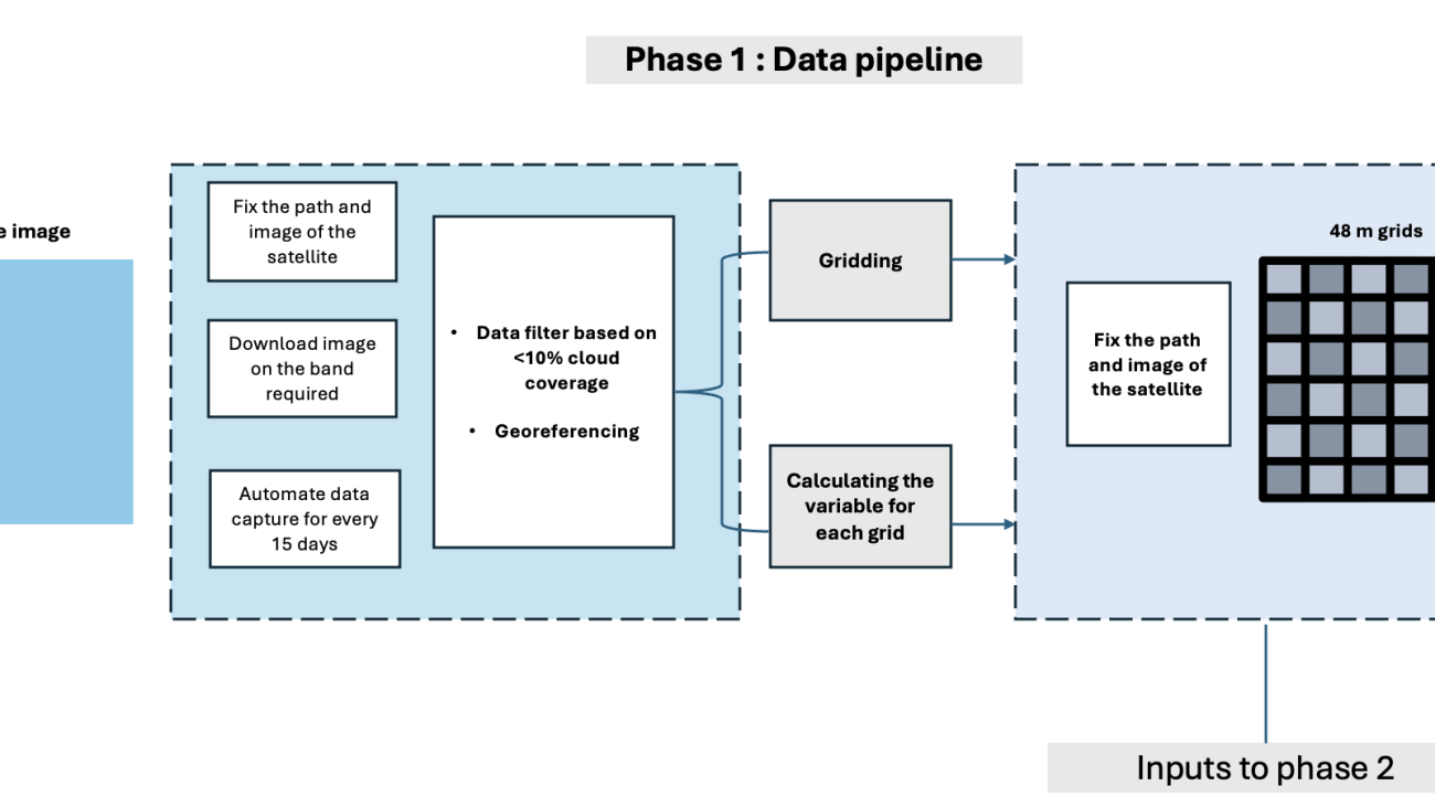
The Landsat 8 satellite captures detailed imagery of the area of interest every 15 days at 11:30 AM, providing a comprehensive view of the city’s landscape and environment. A grid system is established with a 48-meter grid size using Mapbox’s Supermercado Python library at zoom level 19, enabling precise spatial analysis.

Data Pipeline

Phase 2: Exploratory analysis

Integrating infrastructure and population data layers, Geobox empowers users to visualize the city’s variable distribution and derive urban morphological insights, enabling a comprehensive analysis of the city’s structure and development.

Also, Landsat imagery from phase 1 is used to derive insights like the Normalized Difference Vegetation Index (NDVI) and Normalized Difference Built-up Index (NDBI), with data meticulously scaled to the 48-meter grid for consistency and accuracy.

Exploratory Analysis

The following variables are used:

  • Land surface temperature
  • Building site coverage
  • NDVI
  • Building block coverage
  • NDBI
  • Building area
  • Albedo
  • Building count
  • Modified Normalized Difference Water Index (MNDWI)
  • Building height
  • Number of floors and floor area
  • Floor area ratio

Phase 3: Analytics model

This phase comprises three modules, employing ML models on data to gain insights into LST and its relationship with other influential factors:

  • Module 1: Zonal statistics and aggregation – Zonal statistics play a vital role in computing statistics using values from the value raster. It involves extracting statistical data for each zone based on the zone raster. Aggregation is performed at a 100-meter resolution, allowing for a comprehensive analysis of the data.
  • Module 2: Spatial modeling – Gramener evaluated three regression models (linear, spatial, and spatial fixed effects) to unravel the correlation between Land Surface Temperature (LST) and other variables. Among these models, the spatial fixed effect model yielded the highest mean R-squared value, particularly for the timeframe spanning 2014 to 2020.
  • Module 3: Variables forecasting – To forecast variables in the short term, Gramener employed exponential smoothing techniques. These forecasts aided in understanding future LST values and their trends. Additionally, they delved into long-term scale analysis by using Representative Concentration Pathway (RCP8.5) data to predict LST values over extended periods.

Analytics model

Data acquisition and preprocessing

To implement the modules, Gramener used the SageMaker geospatial notebook within Amazon SageMaker Studio. The geospatial notebook kernel is pre-installed with commonly used geospatial libraries, enabling direct visualization and processing of geospatial data within the Python notebook environment.

Gramener employed various datasets to predict LST trends, including building assessment and temperature data, as well as satellite imagery. The key to the UHI solution was using data from the Landsat 8 satellite. This Earth-imaging satellite, a joint venture of USGS and NASA, served as a fundamental component in the project.

With the SearchRasterDataCollection API, SageMaker provides a purpose-built functionality to facilitate the retrieval of satellite imagery. Gramener used this API to retrieve Landsat 8 satellite data for the UHI solution.

The SearchRasterDataCollection API uses the following input parameters:

  • Arn – The Amazon Resource Name (ARN) of the raster data collection used in the query
  • AreaOfInterest – A GeoJSON polygon representing the area of interest
  • TimeRangeFilter – The time range of interest, denoted as {StartTime: <string>, EndTime: <string>}
  • PropertyFilters – Supplementary property filters, such as specifications for maximum acceptable cloud cover, can also be incorporated

The following example demonstrates how Landsat 8 data can be queried via the API:

search_params = {
    "Arn": "arn:aws:sagemaker-geospatial:us-west-2:378778860802:raster-data-collection/public/gmqa64dcu2g9ayx1", # NASA/USGS Landsat
    "RasterDataCollectionQuery": {
        "AreaOfInterest": {
            "AreaOfInterestGeometry": {
                "PolygonGeometry": {
                    "Coordinates": coordinates
                }
            }
        },
        "TimeRangeFilter": {
            "StartTime": "2014-01-01T00:00:00Z",
            "EndTime": "2020-12-31T23:59:59Z",
        },
        "PropertyFilters": {
            "Properties": [{"Property": {"EoCloudCover": {"LowerBound": 0, "UpperBound": 20.0}}}],
            "LogicalOperator": "AND",
        }
    },
}

response = geospatial_client.search_raster_data_collection(**search_params)

To process large-scale satellite data, Gramener used Amazon SageMaker Processing with the geospatial container. SageMaker Processing enables the flexible scaling of compute clusters to accommodate tasks of varying sizes, from processing a single city block to managing planetary-scale workloads. Traditionally, manually creating and managing a compute cluster for such tasks was both costly and time-consuming, particularly due to the complexities involved in standardizing an environment suitable for geospatial data handling.

Now, with the specialized geospatial container in SageMaker, managing and running clusters for geospatial processing has become more straightforward. This process requires minimal coding effort: you simply define the workload, specify the location of the geospatial data in Amazon Simple Storage Service (Amazon S3), and select the appropriate geospatial container. SageMaker Processing then automatically provisions the necessary cluster resources, facilitating the efficient run of geospatial tasks on scales that range from city level to continent level.

Processing

SageMaker fully manages the underlying infrastructure required for the processing job. It allocates cluster resources for the duration of the job and removes them upon job completion. Finally, the results of the processing job are saved in the designated S3 bucket.

A SageMaker Processing job using the geospatial image can be configured as follows from within the geospatial notebook:

from sagemaker import get_execution_role
from sagemaker.sklearn.processing import ScriptProcessor
from sagemaker.processing import ProcessingInput, ProcessingOutput

execution_role_arn = get_execution_role()

geospatial_image_uri = '081189585635.dkr.ecr.us-west-2.amazonaws.com/sagemaker-geospatial-v1-0:latest'
processor = ScriptProcessor(
    command=['python3'],
    image_uri=geospatial_image_uri,
    role=execution_role_arn,
    instance_count=20,
    instance_type='ml.m5.xlarge',
    base_job_name='geospatial-processing-spectral-indices'
)

The instance_count parameter defines how many instances the processing job should use, and the instance_type defines what type of instance should be used.

The following example shows how a Python script is run on the processing job cluster. When the run command is invoked, the cluster starts up and automatically provisions the necessary cluster resources:

processor.run(
    code='calculate_variables.py',
    inputs=[
        ProcessingInput(
            source=s3_manifest_url,
            destination='/opt/ml/processing/input_data/',
            s3_data_type="ManifestFile",
            s3_data_distribution_type="ShardedByS3Key"
        ),
    ],
    outputs=[
        ProcessingOutput(
            source='/opt/ml/processing/output_data/',
            destination=s3_output_prefix_url
        )
    ]
)

Spatial modeling and LST predictions

In the processing job, a range of variables, including top-of-atmosphere spectral radiance, brightness temperature, and reflectance from Landsat 8, are computed. Additionally, morphological variables such as floor area ratio (FAR), building site coverage, building block coverage, and Shannon’s Entropy Value are calculated.

The following code demonstrates how this band arithmetic can be performed:

def calculate_ndvi(nir08, red): 
    return (nir08 - red) / (nir08 + red) 
 
def calculate_ndbi(swir16, nir08): 
    return (swir16 - nir08) / (swir16 + nir08) 
 
def calculate_st(bt): 
    return ((bt * 0.00341802) + 149.0) - 273 
 
def indices_calc(data): 
    with concurrent.futures.ThreadPoolExecutor() as executor: 
        ndvi_future = executor.submit(calculate_ndvi, data.sel(band="SR_B5"), data.sel(band="SR_B4")) 
        ndbi_future = executor.submit(calculate_ndbi, data.sel(band="SR_B6"), data.sel(band="SR_B5")) 
        st_future = executor.submit(calculate_st, data.sel(band="ST_B10")) 
 
        ndvi = ndvi_future.result() 
        ndbi = ndbi_future.result() 
        st = st_future.result() 
 
    ndvi.attrs = data.attrs 
    ndbi.attrs = data.attrs 
    st.attrs = data.attrs 
 
    return ndvi, ndbi, st 

After the variables have been calculated, zonal statistics are performed to aggregate data by grid. This involves calculating statistics based on the values of interest within each zone. For these computations a grid size of approximately 100 meters has been used.

def process_iteration(st, ndvi, ndmi, date, city_name): 
    datacube['st'] = (st.dims, st.values) 
    datacube['ndvi'] = (ndvi.dims, ndvi.values) 
    datacube['ndmi'] = (ndmi.dims, ndmi.values) 
    df = datacube.groupby("id").mean().to_dataframe().reset_index() 
    merged_grid = hexgrid_utm.join(df, on='id', how='left', lsuffix='_')[['id', 'hex_id', 'geometry', 'st', 'ndvi', 'ndmi']] 
    merged_grid.to_file(f"{DATA}/{city_name}/{city_name}_outputs_{date}.geojson", driver='GeoJSON') 
    print("Working on:", date) 
 
def iterative_op(city_json, st, ndvi, ndmi, city_name): 
    with concurrent.futures.ThreadPoolExecutor() as executor: 
        futures = [ 
            executor.submit(process_iteration, st[i], ndvi[i], ndmi[i], date, city_name) 
            for i, _ in enumerate(city_json.time) 
            for date in city_json.date 
        ] 
        for future in concurrent.futures.as_completed(futures): 
            future.result() 
 
    print('Process completed') 

After aggregating the data, spatial modeling is performed. Gramener used spatial regression methods, such as linear regression and spatial fixed effects, to account for spatial dependence in the observations. This approach facilitates modeling the relationship between variables and LST at a micro level.

The following code illustrates how such spatial modeling can be run:

features = [ 
    'ndvi', 
    'ndbi', 
    'st', 
    'build_count', 
    'bbc' 
] 
 
def compute_spatial_weights(df, k=8): 
    knn = KNN.from_dataframe(df, k=k) 
    return df[features].apply(lambda y: weights.spatial_lag.lag_spatial(knn, y)).rename(columns=lambda c: 'w_' + c) 
 
def ordinary_least_squares(df_year, spatial=False): 
    formula = f"lst ~ {' + '.join(features)}"  
    if spatial: 
        df_year = df_year.join(compute_spatial_weights(df_year)) 
        formula += f" + {' + '.join(['w_' + f for f in features])}"  
     
    return smf.ols(formula, data=df_year).fit() 
 
def process(df, year): 
    df_year = pd.merge(df[df['year'] == year].fillna(0), grids[['idx', 'name']], on='idx') 
    ols_model = ordinary_least_squares(df_year) 
    ols_spatial_model = ordinary_least_squares(df_year, spatial=True) 
    ols_spatial_fe_model = ordinary_least_squares(df_year, spatial=True) 
     
    return { 
        'year': year, 
        'ols_model': ols_model, 
        'ols_spatial_model': ols_spatial_model, 
        'ols_spatial_fe_model': ols_spatial_fe_model, 
        'ols_r2': [ols_model.rsquared, ols_spatial_model.rsquared, ols_spatial_fe_model.rsquared] 
    } 

Gramener used exponential smoothing to predict the LST values. Exponential smoothing is an effective method for time series forecasting that applies weighted averages to past data, with the weights decreasing exponentially over time. This method is particularly effective in smoothing out data to identify trends and patterns. By using exponential smoothing, it becomes possible to visualize and predict LST trends with greater precision, allowing for more accurate predictions of future values based on historical patterns.

To visualize the predictions, Gramener used the SageMaker geospatial notebook with open-source geospatial libraries to overlay model predictions on a base map and provides layered visualize geospatial datasets directly within the notebook.

Visualization

Conclusion

This post demonstrated how Gramener is empowering clients to make data-driven decisions for sustainable urban environments. With SageMaker, Gramener achieved substantial time savings in UHI analysis, reducing processing time from weeks to hours. This rapid insight generation allows Gramener’s clients to pinpoint areas requiring UHI mitigation strategies, proactively plan urban development and infrastructure projects to minimize UHI, and gain a holistic understanding of environmental factors for comprehensive risk assessment.

Discover the potential of integrating Earth observation data in your sustainability projects with SageMaker. For more information, refer to Get started with Amazon SageMaker geospatial capabilities.


About the Authors

Abhishek Mittal is a Solutions Architect for the worldwide public sector team with Amazon Web Services (AWS), where he primarily works with ISV partners across industries providing them with architectural guidance for building scalable architecture and implementing strategies to drive adoption of AWS services. He is passionate about modernizing traditional platforms and security in the cloud. Outside work, he is a travel enthusiast.

Janosch Woschitz is a Senior Solutions Architect at AWS, specializing in AI/ML. With over 15 years of experience, he supports customers globally in leveraging AI and ML for innovative solutions and building ML platforms on AWS. His expertise spans machine learning, data engineering, and scalable distributed systems, augmented by a strong background in software engineering and industry expertise in domains such as autonomous driving.

Shravan Kumar is a Senior Director of Client success at Gramener, with decade of experience in Business Analytics, Data Evangelism & forging deep Client Relations. He holds a solid foundation in Client Management, Account Management within the realm of data analytics, AI & ML.

Avirat S is a geospatial data scientist at Gramener, leveraging AI/ML to unlock insights from geographic data. His expertise lies in disaster management, agriculture, and urban planning, where his analysis informs decision-making processes.

Read More

NVIDIA Ranked by Fortune at No. 3 on ‘100 Best Companies to Work For’ List

NVIDIA Ranked by Fortune at No. 3 on ‘100 Best Companies to Work For’ List

NVIDIA jumped to No. 3 on the latest list of America’s 100 Best Companies to Work For by Fortune magazine and Great Place to Work.

It’s the company’s eighth consecutive year and highest ranking yet on the widely followed list, published today, which more than a thousand businesses vie to land on. NVIDIA ranked sixth last year.

“Since the COVID pandemic, employees are increasingly prioritizing work-life balance, mission alignment and empathetic workplaces,” Fortune wrote, with hotelier Hilton taking the top spot, followed by Cisco.

“Even as the broader tech sector has shed tens of thousands of jobs, NVIDIA continued its remarkable streak of nearly 15 years without any layoffs,” Fortune noted in its writeup. NVIDIA also was cited for the company’s “flat structure,” which encourages employees to solve problems quickly and collaboratively through projects.

Survey Says: 97% Are Proud to Share They Work at NVIDIA

To identify the top 100, Fortune conducted a detailed employee survey with Great Place to Work that received more than 1.3 million responses from people in the U.S. The survey showed that 97% of NVIDIANs are proud to tell others where they work.

While many tech companies faced a challenging 2023, with an uncertain economy and several of the biggest employers laying off thousands of workers, NVIDIA focused on managing costs, encouraging innovation and offering unique benefits and compensation that supported employees.

Learn more about NVIDIA life, culture and careers.

Read More

Build a news recommender application with Amazon Personalize

Build a news recommender application with Amazon Personalize

With a multitude of articles, videos, audio recordings, and other media created daily across news media companies, readers of all types—individual consumers, corporate subscribers, and more—often find it difficult to find news content that is most relevant to them. Delivering personalized news and experiences to readers can help solve this problem, and create more engaging experiences. However, delivering truly personalized recommendations presents several key challenges:

  • Capturing diverse user interests – News can span many topics and even within specific topics, readers can have varied interests.
  • Addressing limited reader history – Many news readers have sparse activity histories. Recommenders must quickly learn preferences from limited data to provide value.
  • Timeliness and trending – Daily news cycles mean recommendations must balance personalized content with the discovery of new, popular stories.
  • Changing interests – Readers’ interests can evolve over time. Systems have to detect shifts and adapt recommendations accordingly.
  • Explainability – Providing transparency into why certain stories are recommended builds user trust. The ideal news recommendation system understands the individual and responds to the broader news climate and audience. Tackling these challenges is key to effectively connecting readers with content they find informative and engaging.

In this post, we describe how Amazon Personalize can power a scalable news recommender application. This solution was implemented at a Fortune 500 media customer in H1 2023 and can be reused for other customers interested in building news recommenders.

Solution overview

Amazon Personalize is a great fit to power a news recommendation engine because of its ability to provide real-time and batch personalized recommendations at scale. Amazon Personalize offers a variety of recommendation recipes (algorithms), such as the User Personalization and Trending Now recipes, which are particularly suitable for training news recommender models. The User Personalization recipe analyzes each user’s preferences based on their engagement with content over time. This results in customized news feeds that surface the topics and sources most relevant to an individual user. The Trending Now recipe complements this by detecting rising trends and popular news stories in real time across all users. Combining recommendations from both recipes allows the recommendation engine to balance personalization with the discovery of timely, high-interest stories.

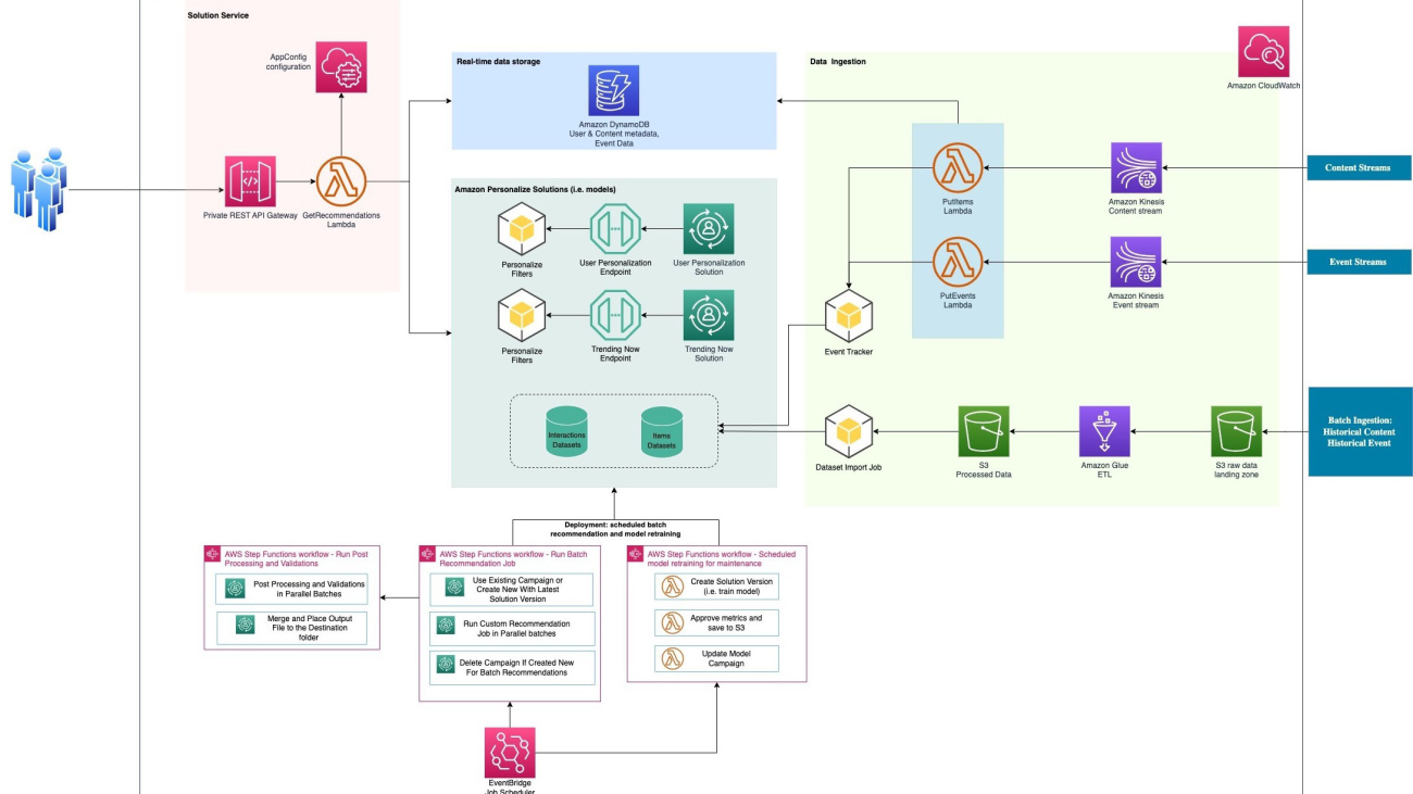
The following diagram illustrates the architecture of a news recommender application powered by Amazon Personalize and supporting AWS services.

This solution has the following limitations:

  • Providing personalized recommendations for just-published articles (articles published a few minutes ago) can be challenging. We describe how to mitigate this limitation later in this post.
  • Amazon Personalize has a fixed number of interactions and items dataset features that can be used to train a model.
  • At the time of writing, Amazon Personalize doesn’t provide recommendation explanations at the user level.

Let’s walk through each of the main components of the solution.

Prerequisites

To implement this solution, you need the following:

  • Historical and real-time user click data for the interactions dataset
  • Historical and real-time news article metadata for the items dataset

Ingest and prepare the data

To train a model in Amazon Personalize, you need to provide training data. In this solution, you use two types of Amazon Personalize training datasets: the interactions dataset and items dataset. The interactions dataset contains data on user-item-timestamp interactions, and the items dataset contains features on the recommended articles.

You can take two different approaches to ingest training data:

  • Batch ingestion – You can use AWS Glue to transform and ingest interactions and items data residing in an Amazon Simple Storage Service (Amazon S3) bucket into Amazon Personalize datasets. AWS Glue performs extract, transform, and load (ETL) operations to align the data with the Amazon Personalize datasets schema. When the ETL process is complete, the output file is placed back into Amazon S3, ready for ingestion into Amazon Personalize via a dataset import job.
  • Real-time ingestion – You can use Amazon Kinesis Data Streams and AWS Lambda to ingest real-time data incrementally. A Lambda function performs the same data transformation operations as the batch ingestion job at the individual record level, and ingests the data into Amazon Personalize using the PutEvents and PutItems APIs.

In this solution, you can also ingest certain items and interactions data attributes into Amazon DynamoDB. You can use these attributes during real-time inference to filter recommendations by business rules. For example, article metadata may contain company and industry names in the article. To proactively recommend articles on companies or industries that users are reading about, you can record how frequently readers are engaging with articles about specific companies and industries, and use this data with Amazon Personalize filters to further tailor the recommended content. We discuss more about how to use items and interactions data attributes in DynamoDB later in this post.

The following diagram illustrates the data ingestion architecture.

Train the model

The bulk of the model training effort should focus on the User Personalization model, because it can use all three Amazon Personalize datasets (whereas the Trending Now model only uses the interactions dataset). We recommend running experiments that systematically vary different aspects of the training process. For the customer that implemented this solution, the team ran over 30 experiments. This included modifying the interactions and items dataset features, adjusting the length of interactions history provided to the model, tuning Amazon Personalize hyperparameters, and evaluating whether an explicit user’s dataset improved offline performance (relative to the increase in training time).

Each model variation was evaluated based on metrics reported by Amazon Personalize on the training data, as well as custom offline metrics on a holdout test dataset. Standard metrics to consider include mean average precision (MAP) @ K (where K is the number of recommendations presented to a reader), normalized discounted cumulative gain, mean reciprocal rank, and coverage. For more information about these metrics, see Evaluating a solution version with metrics. We recommend prioritizing MAP @ K out of these metrics, which captures the average number of articles a reader clicked on out of the top K articles recommended to them, because the MAP metric is a good proxy for (real) article clickthrough rates. K should be selected based on the number of articles a reader can view on a desktop or mobile webpage without having to scroll, allowing you to evaluate recommendation effectiveness with minimal reader effort. Implementing custom metrics, such as recommendation uniqueness (which describes how unique the recommendation output was across the pool of candidate users), can also provide insight into recommendation effectiveness.

With Amazon Personalize, the experimental process allows you to determine the optimal set of dataset features for both the User Personalization and Trending Now models. The Trending Now model exists within the same Amazon Personalize dataset group as the User Personalization model, so it uses the same set of interactions dataset features.

Generate real-time recommendations

When a reader visits a news company’s webpage, an API call will be made to the news recommender via Amazon API Gateway. This triggers a Lambda function that calls the Amazon Personalize models’ endpoints to get recommendations in real time. During inference, you can use filters to filter the initial recommendation output based on article or reader interaction attributes. For example, if “News Topic” (such as sports, lifestyle, or politics) is an article attribute, you can restrict recommendations to specific news topics if that is a product requirement. Similarly, you can use filters on reader interaction events, such as excluding articles a reader has already read.

One key challenge with real-time recommendations is effectively including just-published articles (also called cold items) into the recommendation output. Just-published articles don’t have any historical interaction data that recommenders normally rely on, and recommendation systems need sufficient processing time to assess how relevant just-published articles are to a specific user (even if only using user-item relationship signals).

Amazon Personalize can natively auto detect and recommend new articles ingested into the items dataset every 2 hours. However, because this use case is focused on news recommendations, you need a way to recommend new articles as soon as they’re published and ready for reader consumption.

One way to solve this problem is by designing a mechanism to randomly insert just-published articles into the final recommendation output for each reader. You can add a feature to control what percent of articles in the final recommendation set were just-published articles, and similar to the original recommendation output from Amazon Personalize, you can filter just-published articles by article attributes (such as “News Topic”) if it is a product requirement. You can track interactions on just-published articles in DynamoDB as they start trickling in to the system, and prioritize the most popular just-published articles during recommendation postprocessing, until the just-published articles are detected and processed by the Amazon Personalize models.

After you have your final set of recommended articles, this output is submitted to another postprocessing Lambda function that checks the output to see if it aligns with pre-specified business rules. These can include checking whether recommended articles meet webpage layout specifications, if recommendations are served in a web browser frontend, for example. If needed, articles can be reranked to ensure business rules are met. We recommend reranking by implementing a function that allows higher-ranking articles to only fall down in ranking one place at a time until all business rules are met, providing minimal relevancy loss for readers. The final list of postprocessed articles is returned to the web service that initiated the request for recommendations.

The following diagram illustrates the architecture for this step in the solution.

Generate batch recommendations

Personalized news dashboards (through real-time recommendations) require a reader to actively search for news, but in our busy lives today, sometimes it’s just easier to have your top news sent to you. To deliver personalized news articles as an email digest, you can use an AWS Step Functions workflow to generate batch recommendations. The batch recommendation workflow gathers and postprocesses recommendations from our User Personalization model or Trending Now model endpoints, giving flexibility to select what combination of personalized and trending articles teams want to push to their readers. Developers also have the option of using the Amazon Personalize batch inference feature; however, at the time of writing, creating an Amazon Personalize batch inference job doesn’t support including items ingested after an Amazon Personalize custom model has been trained, and it doesn’t support the Trending Now recipe.

During a batch inference Step Functions workflow, the list of readers is divided into batches, processed in parallel, and submitted to a postprocessing and validation layer before being sent to the email generation service. The following diagram illustrates this workflow.

Scale the recommender system

To effectively scale, you also need the news recommender to accommodate a growing number of users and increased traffic without creating any degradation in reader experience. Amazon Personalize model endpoints natively auto scale to meet increased traffic. Engineers only need to set and monitor a minimum provisioned transactions per second (TPS) variable for each Amazon Personalize endpoint.

Beyond Amazon Personalize, the news recommender application presented here is built using serverless AWS services, allowing engineering teams to focus on delivering the best reader experience without worrying about infrastructure maintenance.

Conclusion

In this attention economy, it has become increasingly important to deliver relevant and timely content for consumers. In this post, we discussed how you can use Amazon Personalize to build a scalable news recommender, and the strategies organizations can implement to address the unique challenges of delivering news recommendations.

To learn more about Amazon Personalize and how it can help your organization build recommendation systems, check out the Amazon Personalize Developer Guide.

Happy building!


About the Authors

Bala Krishnamoorthy is a Senior Data Scientist at AWS Professional Services, where he helps customers build and deploy AI-powered solutions to solve their business challenges. He has worked with customers across diverse sectors, including media & entertainment, financial services, healthcare, and technology. In his free time, he enjoys spending time with family/friends, staying active, trying new restaurants, travel, and kickstarting his day with a steaming hot cup of coffee.

Rishi Jala is a NoSQL Data Architect with AWS Professional Services. He focuses on architecting and building highly scalable applications using NoSQL databases such as Amazon DynamoDB. Passionate about solving customer problems, he delivers tailored solutions to drive success in the digital landscape.
Read More

Nielsen Sports sees 75% cost reduction in video analysis with Amazon SageMaker multi-model endpoints

Nielsen Sports sees 75% cost reduction in video analysis with Amazon SageMaker multi-model endpoints

This is a guest post co-written with Tamir Rubinsky and Aviad Aranias from Nielsen Sports.

Nielsen Sports shapes the world’s media and content as a global leader in audience insights, data, and analytics. Through our understanding of people and their behaviors across all channels and platforms, we empower our clients with independent and actionable intelligence so they can connect and engage with their audiences—now and into the future.

At Nielsen Sports, our mission is to provide our customers—brands and rights holders—with the ability to measure the return on investment (ROI) and effectiveness of a sport sponsorship advertising campaign across all channels, including TV, online, social media, and even newspapers, and to provide accurate targeting at local, national, and international levels.

In this post, we describe how Nielsen Sports modernized a system running thousands of different machine learning (ML) models in production by using Amazon SageMaker multi-model endpoints (MMEs) and reduced operational and financial cost by 75%.

Challenges with channel video segmentation

Our technology is based on artificial intelligence (AI) and specifically computer vision (CV), which allows us to track brand exposure and identify its location accurately. For example, we identify if the brand is on a banner or a shirt. In addition, we identify the location of the brand on the item, such as the top corner of a sign or the sleeve. The following figure shows an example of our tagging system.

example of Nielsen tagging system

To understand our scaling and cost challenges, let’s look at some representative numbers. Every month, we identify over 120 million brand impressions across different channels, and the system must support the identification of over 100,000 brands and variations of different brands. We have built one of the largest databases of brand impressions in the world with over 6 billion data points.

Our media evaluation process includes several steps, as illustrated in the following figure:

  1. First, we record thousands of channels around the world using an international recording system.
  2. We stream the content in combination with the broadcast schedule (Electronic Programming Guide) to the next stage, which is segmentation and separation between the game broadcasts themselves and other content or advertisements.
  3. We perform media monitoring, where we add additional metadata to each segment, such as league scores, relevant teams, and players.
  4. We perform an exposure analysis of the brands’ visibility and then combine the audience information to calculate the valuation of the campaign.
  5. The information is delivered to the customer by a dashboard or analyst reports. The analyst is given direct access to the raw data or through our data warehouse.

media evaluation steps

Because we operate at a scale of over a thousand channels and tens of thousands of hours of video a year, we must have a scalable automation system for the analysis process. Our solution automatically segments the broadcast and knows how to isolate the relevant video clips from the rest of the content.

We do this using dedicated algorithms and models developed by us for analyzing the specific characteristics of the channels.

In total, we are running thousands of different models in production to support this mission, which is costly, incurs operational overhead, and is error-prone and slow. It took months to get models with new model architecture to production.

This is where we wanted to innovate and rearchitect our system.

Cost-effective scaling for CV models using SageMaker MMEs

Our legacy video segmentation system was difficult to test, change, and maintain. Some of the challenges include working with an old ML framework, inter-dependencies between components, and a hard-to-optimize workflow. This is because we were based on RabbitMQ for the pipeline, which was a stateful solution. To debug one component, such as feature extraction, we had to test all of the pipeline.

The following diagram illustrates the previous architecture.

previous architecture

As part of our analysis, we identified performance bottlenecks such as running a single model on a machine, which showed a low GPU utilization of 30–40%. We also discovered inefficient pipeline runs and scheduling algorithms for the models.

Therefore, we decided to build a new multi-tenant architecture based on SageMaker, which would implement performance optimization improvements, support dynamic batch sizes, and run multiple models simultaneously.

Each run of the workflow targets a group of videos. Each video is between 30–90 minutes long, and each group has more than five models to run.

Let’s examine an example: a video can be 60 minutes long, consisting of 3,600 images, and each image needs to inferred by three different ML models during the first stage. With SageMaker MMEs, we can run batches of 12 images in parallel, and the full batch completes in less than 2 seconds. In a regular day, we have more than 20 groups of videos, and on a packed weekend day, we can have more than 100 groups of videos.

The following diagram shows our new, simplified architecture using a SageMaker MME.

simplified architecture using a SageMaker MME

Results

With the new architecture, we achieved many of our desired outcomes and some unseen advantages over the old architecture:

  • Better runtime – By increasing batch sizes (12 videos in parallel) and running multiple models concurrently (five models in parallel), we have decreased our overall pipeline runtime by 33%, from 1 hour to 40 minutes.
  • Improved infrastructure – With SageMaker, we upgraded our existing infrastructure, and we are now using newer AWS instances with newer GPUs such as g5.xlarge. One of the biggest benefits from the change is the immediate performance improvement from using TorchScript and CUDA optimizations.
  • Optimized infrastructure usage – By having a single endpoint that can host multiple models, we can reduce both the number of endpoints and the number of machines we need to maintain, and also increase the utilization of a single machine and its GPU. For a specific task with five videos, we now use only five machines of g5 instances, which gives us 75% cost benefit from the previous solution. For a typical workload during the day, we use a single endpoint with a single machine of g5.xlarge with a GPU utilization of more than 80%. For comparison, the previous solution had less than 40% utilization.
  • Increased agility and productivity – Using SageMaker allowed us to spend less time migrating models and more time improving our core algorithms and models. This has increased productivity for our engineering and data science teams. We can now research and deploy a new ML model in under 7 days, instead of over 1 month previously. This is a 75% improvement in velocity and planning.
  • Better quality and confidence – With SageMaker A/B testing capabilities, we can deploy our models in a gradual way and be able to safely roll back. The faster lifecycle to production also increased our ML models’ accuracy and results.

The following figure shows our GPU utilization with the previous architecture (3040% GPU utilization).

GPU utilization with the previous architecture

The following figure shows our GPU utilization with the new simplified architecture (90% GPU utilization).

GPU utilization with the new simplified architecture

Conclusion

In this post, we shared how Nielsen Sports modernized a system running thousands of different models in production by using SageMaker MMEs and reduced their operational and financial cost by 75%.

For further reading, refer to the following:


About the Authors

Eitan SelaEitan Sela is a Generative AI and Machine Learning Specialist Solutions Architect with Amazon Web Services. He works with AWS customers to provide guidance and technical assistance, helping them build and operate Generative AI and Machine Learning solutions on AWS. In his spare time, Eitan enjoys jogging and reading the latest machine learning articles.

Gal GoldmanGal Goldman is a Senior Software Engineer and an Enterprise Senior Solution Architect in AWS with a passion for cutting-edge solutions. He specializes in and has developed many distributed Machine Learning services and solutions. Gal also focuses on helping AWS customers accelerate and overcome their engineering and Generative AI challenges.

Tal PanchekTal Panchek is a Senior Business Development Manager for Artificial Intelligence and Machine Learning with Amazon Web Services. As a BD Specialist, he is responsible for growing adoption, utilization, and revenue for AWS services. He gathers customer and industry needs and partner with AWS product teams to innovate, develop, and deliver AWS solutions.

Tamir RubinskyTamir Rubinsky leads Global R&D Engineering at Nielsen Sports, bringing vast experience in building innovative products and managing high-performing teams. His work transformed sports sponsorship media evaluation through innovative, AI-powered solutions.

Aviad AraniasAviad Aranias is a MLOps Team Leader and Nielsen Sports Analysis Architect who specializes in crafting complex pipelines for analyzing sports event videos across numerous channels. He excels in building and deploying deep learning models to handle large-scale data efficiently. In his spare time, he enjoys baking delicious Neapolitan pizzas.
Read More

‘The Elder Scrolls Online’ Joins GeForce NOW for Game’s 10th Anniversary

‘The Elder Scrolls Online’ Joins GeForce NOW for Game’s 10th Anniversary

Rain or shine, a new month means new games. GeForce NOW kicks off April with nearly 20 new games, seven of which are available to play this week.

GFN Thursday celebrates the 10-year anniversary of ZeniMax Online Studios’ Elder Scrolls Online by bringing the award-winning online role-playing game (RPG) to the cloud this week.

Plus, the GeForce NOW Ultimate membership comes to gamers in Japan for the first time, with new GeForce RTX 4080 SuperPODs online today.

The Rising Sun Goes Ultimate

Japan and GeForce NOW
Get ready to drift into the cloud.

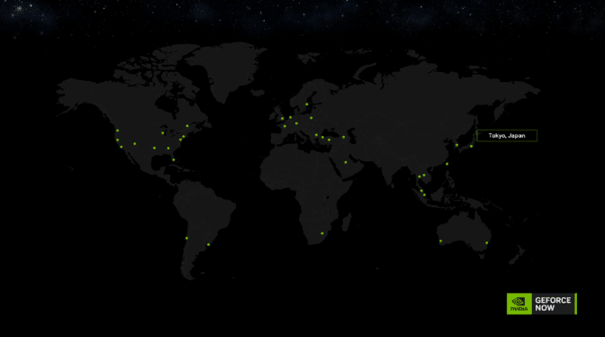
GeForce NOW is rolling out the green carpet to gamers in Japan, expanding next-generation cloud gaming worldwide. The Ultimate membership tier is now available to gamers in the region, delivering up to 4K gaming at up to 120 frames per second, all at ultra-low latency — even on devices without the latest hardware.

Gamers in Japan can now access from the cloud triple-A titles by some of the world’s largest publishers. Capcom’s Street Fighter 6 and Resident Evil Village will be coming to GeForce NOW at a later date for members to stream at the highest performance.

GeForce NOW will operate in Japan alongside GeForce NOW Alliance partner and telecommunications company KDDI, which currently offers its customers access to GeForce RTX 3080-powered servers, in addition to its mobile benefits. Plus, new GFNA partners in other regions will be announced this year — stay tuned to GFN Thursdays for details.

A Decade of Adventure

Elder Scrolls Online on GeForce NOW
The cloud is slay-ing.

Discover Tamriel from the comfort of almost anywhere with GeForce NOW. Explore the Elder Scrolls universe solo or alongside thousands of other players in The Elder Scrolls Online as it joins the cloud this week for members.

For a decade, Elder Scrolls Online has cultivated a vibrant community of millions of players and a legacy of exciting stories, characters and adventures. Players have explored Morrowind, Summerset, Skyrim and more, thanks to regular updates and chapter releases. The title’s anniversary celebrations kick off in Amsterdam this week, and fans worldwide can join in by streaming the game from the cloud.

Set during Tamriel’s Second Era, a millennium before The Elder Scrolls V: Skyrim, The Elder Scrolls Online has players exploring a massive, ever-growing world. Together they can encounter memorable quests, challenging dungeons, player vs. player battles and more. Gamers can play their way by customizing their characters, looting and crafting new gear, and unlocking and developing their abilities.

Experience the epic RPG with an Ultimate membership and venture forth in the cloud with friends, tapping eight-hour gaming sessions and exclusive access to servers. Ultimate members can effortlessly explore the awe-inspiring fantasy world with the ability to stream at up to 4K and 120 fps, or experience the game at ultrawide resolutions on supported devices.

April Showers Bring New Games

MEGAMAN X DiVE OFFLINE on GeForce NOW
X marks the cloud.

Dive into a new adventure with Mega Man X DiVE Offline from Capcom. It’s the offline, reimagined version of Mega Man X, featuring the franchise’s classic action, over 100 characters from the original series and an all-new story with hundreds of stages to play. Strengthen characters and weapons with a variety of power-ups — then test them out in the side-scrolling action.

Catch it alongside other new games joining the cloud this week:

  • ARK: Survival Ascended (New release on Xbox, available on PC Game Pass, April 1)
  • Thief (New release on Epic Games Store, free from April 4-11)
  • Sons of Valhalla (New release on Steam, April 5)
  • Elder Scrolls Online (Steam and Epic Games Store)
  • MEGA MAN X DiVE Offline (Steam)
  • SUPERHOT: MIND CONTROL DELETE (Xbox, available on PC Game Pass)
  • Turbo Golf Racing 1.0 (Xbox, available on PC Game Pass)

And members can look for the following throughout the rest of the month:

  • Dead Island 2 (New release on Steam, April 22)
  • Phantom Fury (New release on Steam, April 23)
  • Oddsparks: An Automation Adventure (New release on Steam, April 24)
  • 9-Bit Armies: A Bit Too Far (Steam)
  • Backpack Battles (Steam)
  • Dragon’s Dogma 2 Character Creator & Storage (Steam)
  • Evil West (Xbox, available on PC Game Pass)
  • Islands of Insight (Steam)
  • Lightyear Frontier (Steam and Xbox, available on PC Game Pass)
  • Manor Lords (New release on Steam and Xbox, available on PC Game Pass)
  • Metaball (Steam)
  • Tortuga – A Pirate’s Tale (Steam)

Making the Most of March

In addition to the 30 games announced last month, six more joined the GeForce NOW library:

  • Zoria: Age of Shattering (New release on Steam, March 7)
  • Deus Ex: Mankind Divided (New release on Epic Games Store, free, March 14)
  • Dragon’s Dogma 2 (New release on Steam, March 21)
  • Diablo IV (Xbox, available on PC Game Pass)
  • Granblue Fantasy: Relink (Steam)
  • Space Engineers (Xbox, available on PC Game Pass)

Some titles didn’t make it in March. Crown Wars: The Black Prince and Breachway have delayed their launch dates to later this year, and Portal: Revolution will join GeForce NOW in the future. Stay tuned to GFN Thursday for updates.

What are you planning to play this weekend? Let us know on X or in the comments below.

Read More

Accelerating MoE model inference with Locality-Aware Kernel Design

Accelerating MoE model inference with Locality-Aware Kernel Design

1.0 Summary

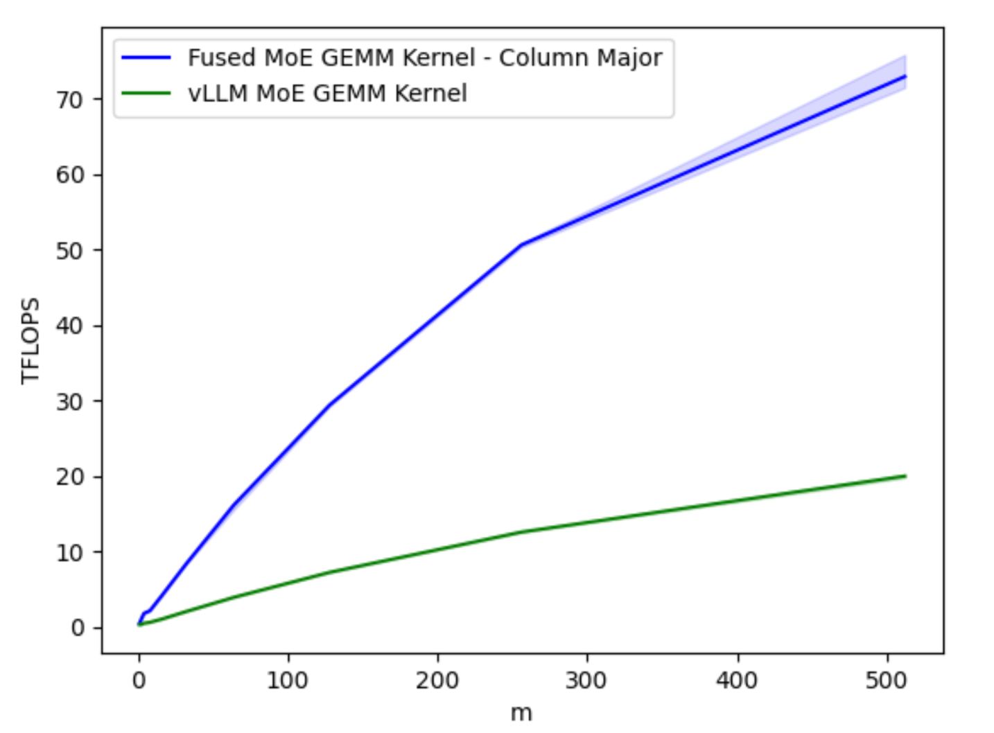
We show that by implementing column-major scheduling to improve data locality, we can accelerate the core Triton GEMM (General Matrix-Matrix Multiply) kernel for MoEs (Mixture of Experts) up to 4x on A100, and up to 4.4x on H100 Nvidia GPUs. This post demonstrates several different work decomposition and scheduling algorithms for MoE GEMMs and shows, at the hardware level, why column-major scheduling produces the highest speedup.

Repo and code available at: https://github.com/pytorch-labs/applied-ai/tree/main/triton/.

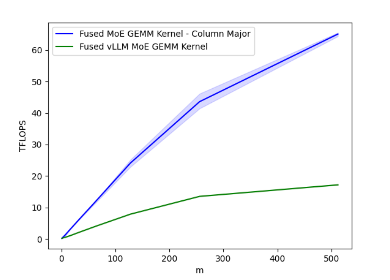
Figure 1A. Optimized Fused MoE GEMM Kernel TFLOPs on A100 for varying Batch Sizes M

Figure 1A. Optimized Fused MoE GEMM Kernel TFLOPs on A100 for varying Batch Sizes M

Figure 1B. Optimized Fused MoE GEMM Kernel TFLOPs on H100 for varying Batch Sizes M

Figure 1B. Optimized Fused MoE GEMM Kernel TFLOPs on H100 for varying Batch Sizes M

2.0 Background

OpenAI’s Triton is a hardware-agnostic language and compiler that as our prior blog post has shown can be used to accelerate quantization workflows. We also showed that in terms of kernel development, much of the same learnings and performance analysis tools from CUDA can be leveraged to provide similar insights into how Triton kernels work under-the-hood and subsequent measures to speedup these kernels in latency sensitive environments. As Triton becomes increasingly adopted in production settings, it is important that developers understand the common tips and tricks to developing performant kernels as well as the generality of these methods to various different architectures and workflows. Thus, this post will explore how we optimized the Triton kernel developed by vLLM for the popular Mixture of Experts (MoE) Mixtral model using classical techniques and how these techniques can be implemented in Triton to achieve performance gain.

Mixtral 8x7B is a sparse Mixture of Experts Language Model. Unlike the classical dense transformer architecture, each transformer block houses 8 MLP layers where each MLP is an ‘expert’. As a token flows through, a router network selects which 2 of the 8 experts should process that token and the results are then combined. The selected experts for the same token vary at each layer. As a result, while Mixtral 8x7B has a total of 47B params, during inference only 13B params are active.

The MoE GEMM (General Matrix-Matrix Multiply) kernel receives a stacked weight matrix containing all the experts, and must subsequently route each token to the TopK (2 for Mixtral) experts by utilizing a mapping array produced by the resultant scores of the router network. In this post, we provide methods to efficiently parallelize this computation during inference time, specifically during autoregression (or decoding stages).

3.0 Work Decomposition – SplitK

We have previously shown that for the matrix problem sizes found in LLM inference, specifically in the context of W4A16 quantized inference, GEMM kernels can be accelerated by applying a SplitK work decomposition. Thus, we started our MoE acceleration research by implementing SplitK in the vLLM MoE Kernel, which produced speedups of approximately 18-20% over the Data Parallel approach.

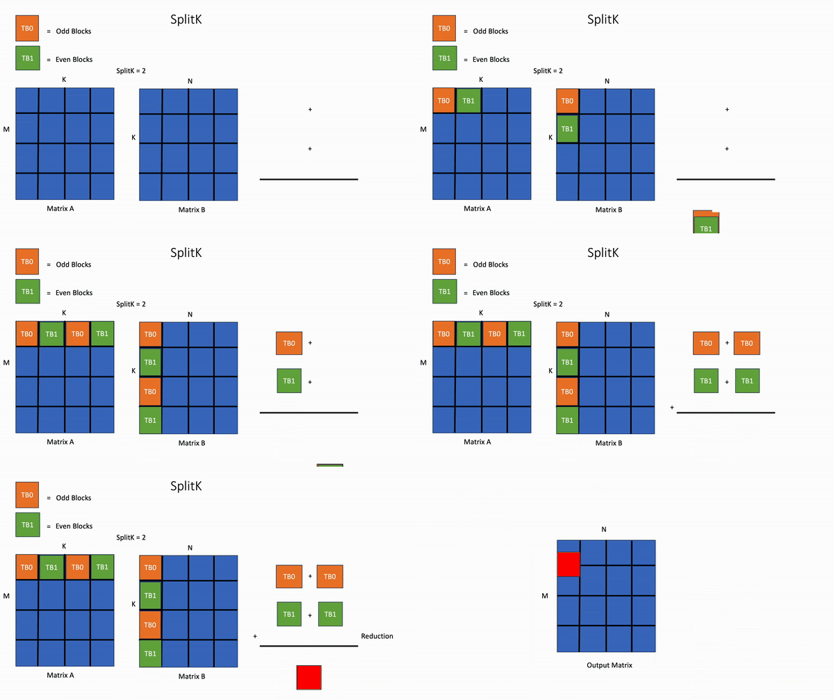
This result shows that the SplitK optimization can be used as a part of a more formulaic approach to improving/developing Triton kernels in inference settings. To build intuition about these different work decompositions, let’s consider a simple example for the multiplication of two 4×4 matrices and SplitK=2.

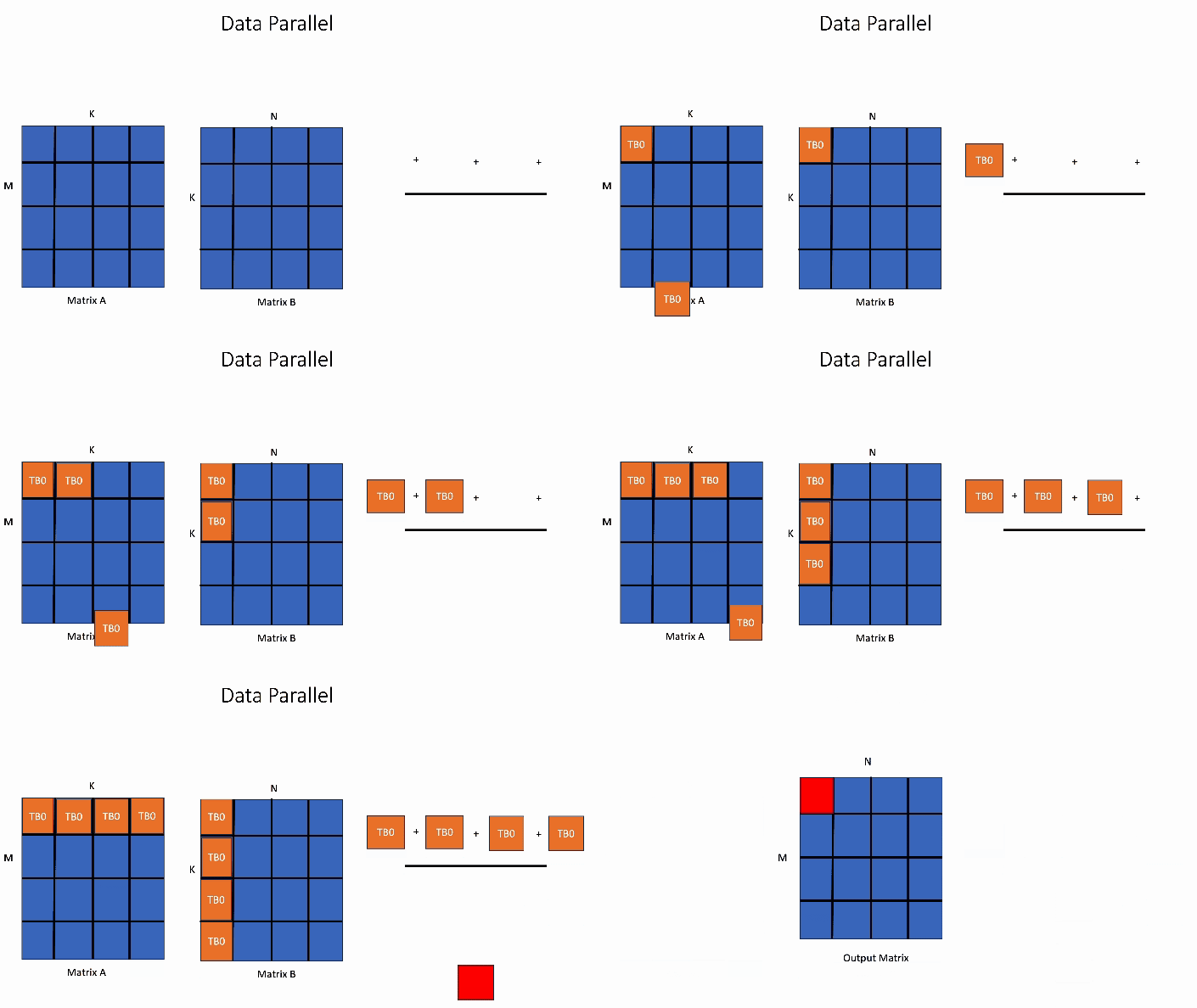
In the data parallel GEMM kernel shown below, the computation for a single block of the output matrix will be handled by 1 threadblock, TB0.

Figure 2. Data Parallel GEMM

Figure 2. Data Parallel GEMM

In contrast, in the SplitK kernel, the work required to compute 1 block in the output matrix, is “split” or shared amongst 2 thread blocks TB0 and TB1. This provides better load balancing and increased parallelism.

Figure 3. SplitK GEMM

Figure 3. SplitK GEMM

The key idea is that we’ve increased our parallelism from MN to MN*SplitK. This approach does incur some costs such as adding inter-threadblock communication via atomic operations. However, these costs are minimal compared to the savings of other constrained GPU resources like shared memory and registers. Most importantly, the SplitK strategy provides superior load balancing characteristics for skinny matrices, (as is the case in MoE inference) and is the common matrix profile during decoding and inference.

4.0 GEMM Hardware Scheduling – Column Major

To improve upon the ~20% speedup with SplitK we focused our investigation on the logic that controls the hardware scheduling of the GEMM in Triton Kernels. Our profiling of the vLLM MoE kernel showed a low L2 cache hit rate, thus we investigated three scheduling options – column-major, row-major and grouped launch. Due to some intrinsic properties of MoE models, such as large expert matrices, and having to dynamically load TopK (2 for Mixtral) matrices during the duration of the kernel, cache reuse/hit rate becomes a bottleneck that this optimization will target.

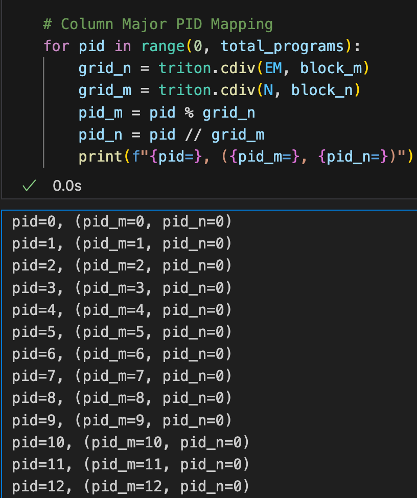
For background, in our previous blog, we touched on the concept of “tile swizzling”, a method to achieve greater L2 cache hit rate. This concept relates to how the software schedules the GEMM onto the SMs of a GPU. In Triton, this schedule is determined by the pid_m and pid_n calculations. Our key insight is that for skinny matrix multiplications, a column-major ordering ensures optimal reuse of the columns of the weight matrix, B. To illustrate this, let’s take a look at a snippet of what a column major computation of pid_m, and pid_n would look like:

Figure 4. Column Major ordering in PyTorch

Figure 4. Column Major ordering in PyTorch

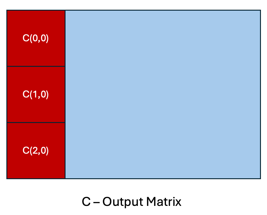
From above, we note that with this mapping, we schedule the GEMM such that we calculate the output blocks of C in the following order: C(0, 0), C(1, 0), C(2, 0),… etc. To understand the implications we provide the following illustration:

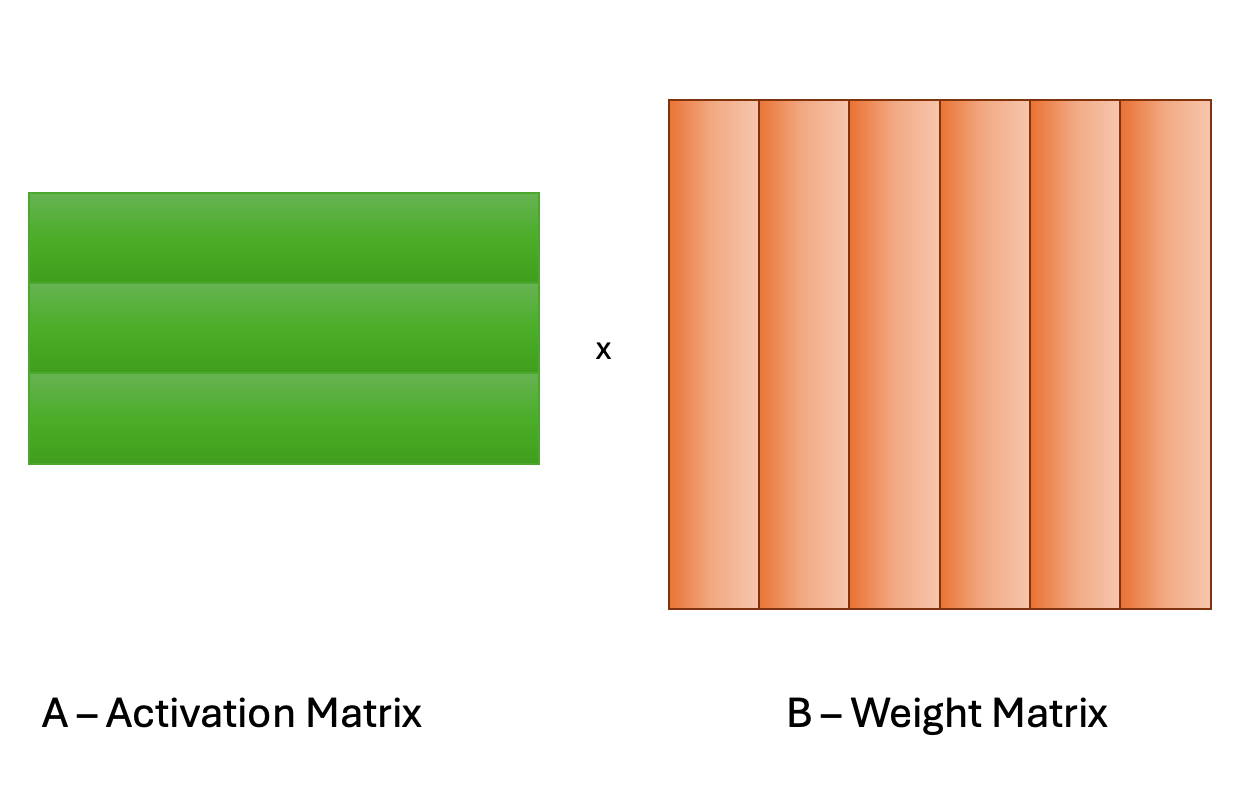
Activation matrix / Weight matrix

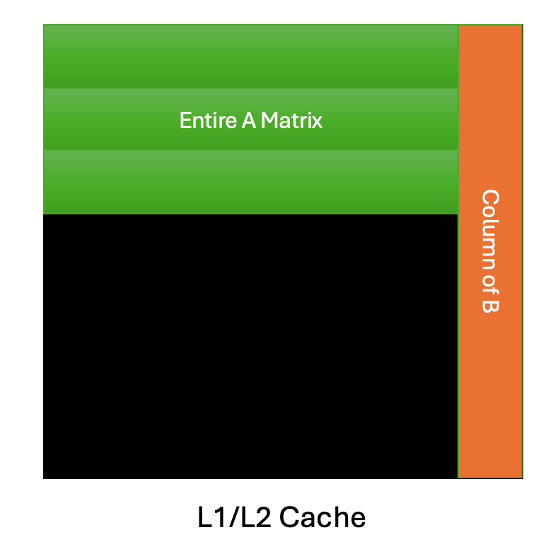
L1/L2 Cache

C - Output Matrix

Figure 5. Cache Reuse Pattern for a Column-Major GEMM Schedule

In the above simplified view of a column-major schedule, let’s assume for a GEMM with skinny activation matrix A, that the entire matrix can fit in the GPU cache which is a reasonable assumption to make for the type of problem sizes we encounter in MoE inference. This allows for maximal reuse of the columns of the weight matrix B, due to the fact that the B column can be re-used for the corresponding output tile calculations, C(0,0), C(1, 0) and C(2, 0). Consider instead, a row-major schedule, C(0,0), C(0,1), C(0, 2) etc. We would have to evict the column of B, and issue multiple load instructions to DRAM to calculate the same amount of output blocks.

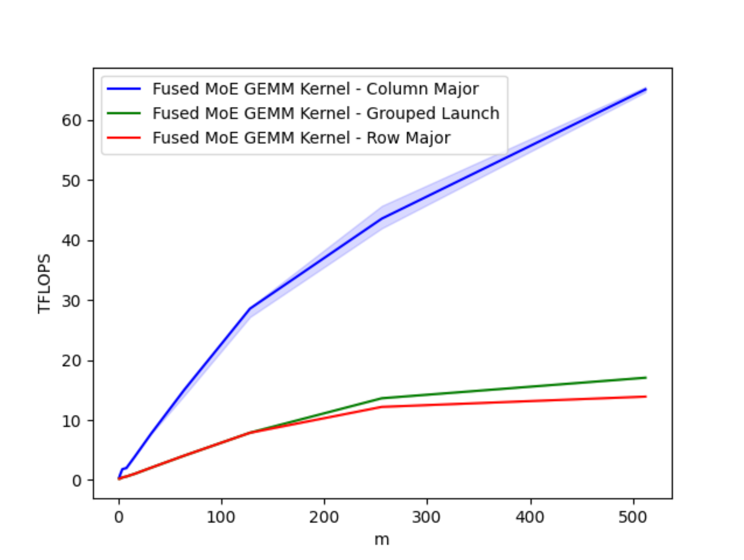
An important design consideration when optimizing kernels is a memory access pattern that results in the least amount of global load instructions. This optimal memory access pattern is achieved with the column-major schedule. The results below showcase the performance of the three schedules we investigated:

Figure 6. Comparison of GEMM Schedules on A100 for varying Batch Sizes M

Figure 6. Comparison of GEMM Schedules on A100 for varying Batch Sizes M

The column-major schedule provides up to a 4x speedup over the other patterns, and as we’ll show in the next section, provides an optimal memory access pattern due to greatly improved data locality.

5.0 Nsight Compute Analysis – Throughput and Memory Access Pattern

For performance analysis, we focus on the M = 2 case for the H100. A similar study can be done for the A100 as many of the same observations carry over. We note the following salient results, that showcase the impact of our optimizations.

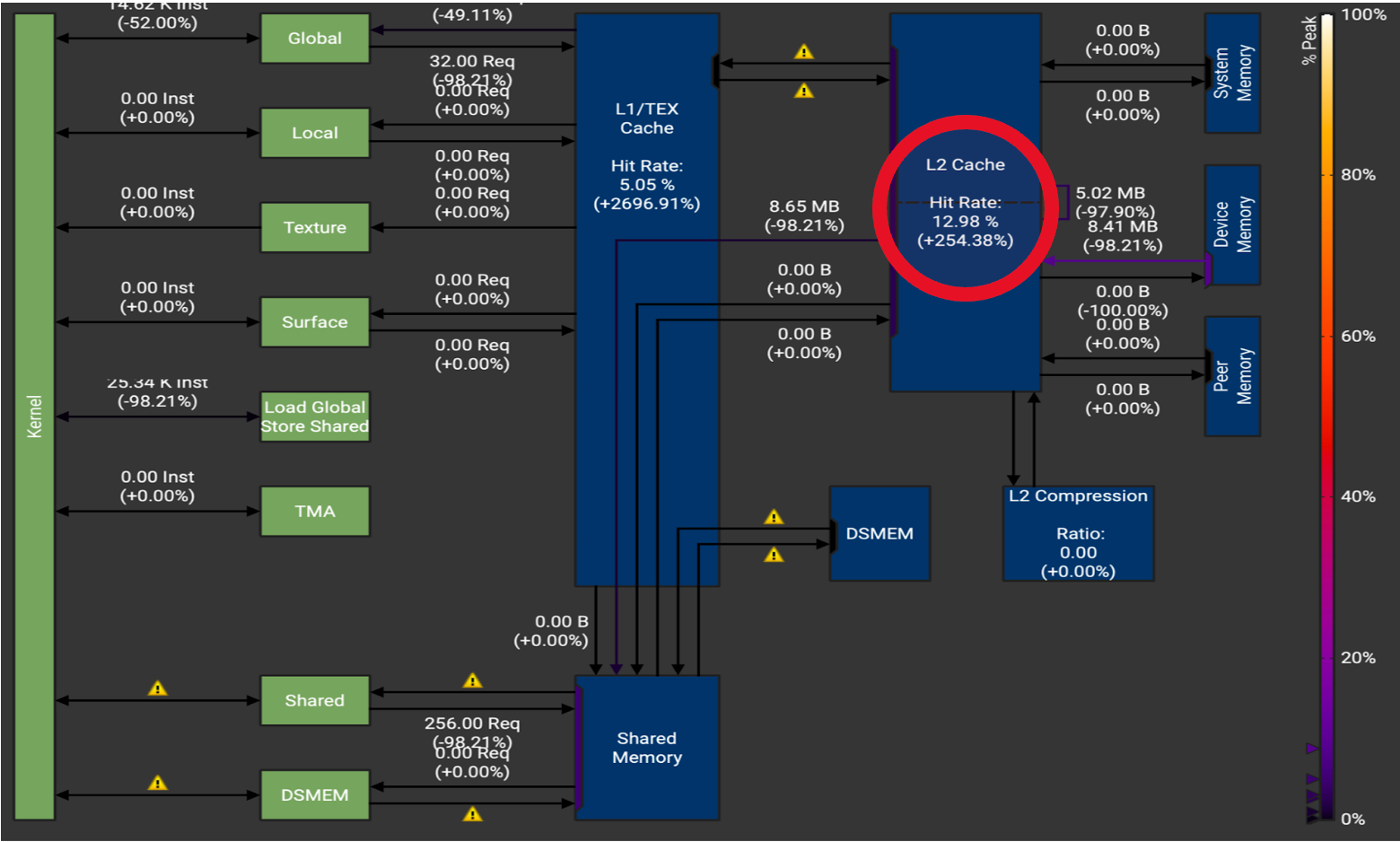
Figure 7. H100 Memory Throughput Chart for M = 2.  Note the very large increase in the cache hit rates L1 cache hit rate (+2696%) and L2 cache hit rate (+254%).

Figure 7. H100 Memory Throughput Chart for M = 2. Note the very large increase in the cache hit rates L1 cache hit rate (+2696%) and L2 cache hit rate (+254%).

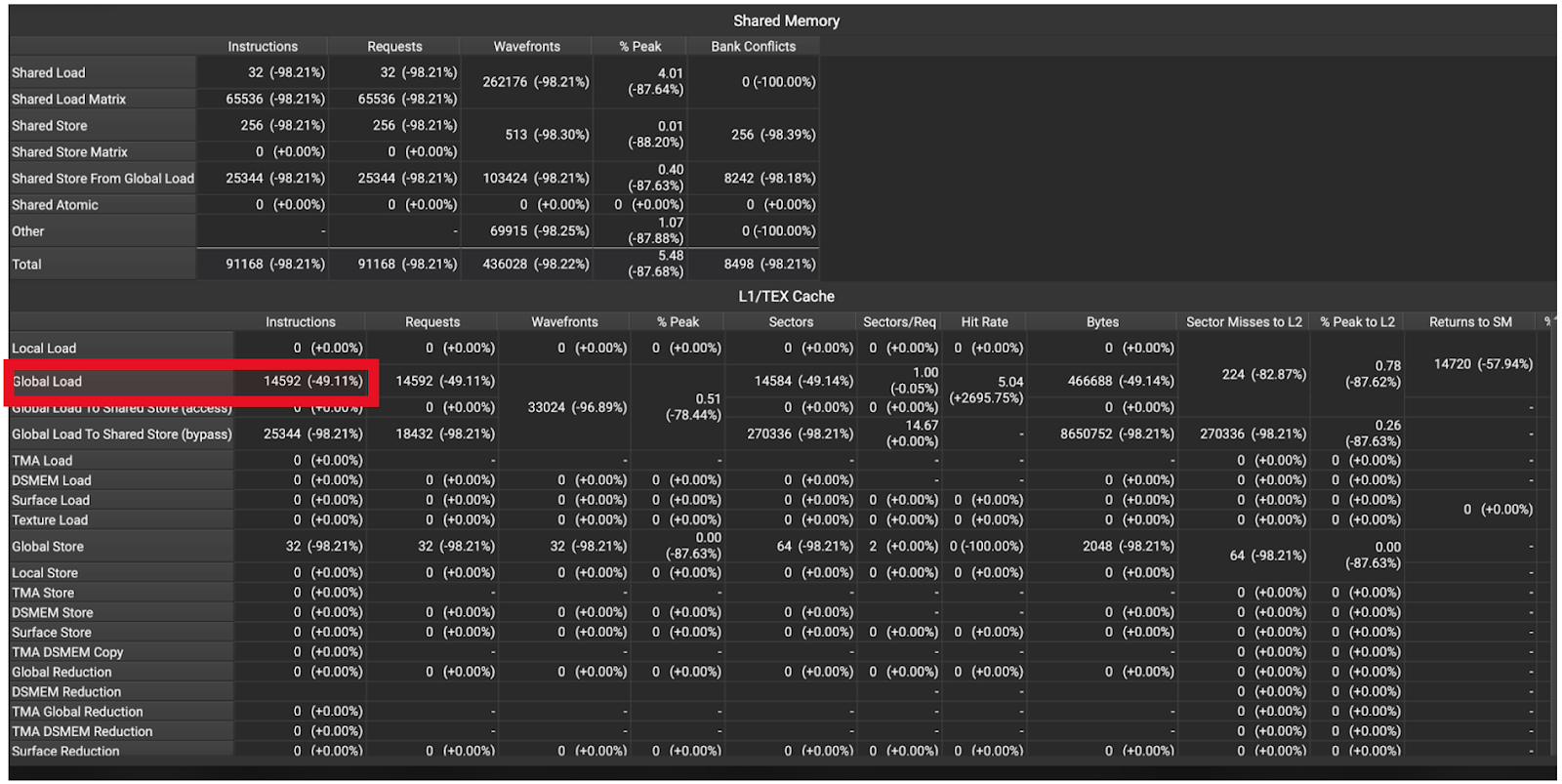
Figure 8. H100 Memory Instruction Statistics M = 2. Note the 49% reduction in global memory loads.

Figure 8. H100 Memory Instruction Statistics M = 2. Note the 49% reduction in global memory loads.

These statistics show that our optimizations had the intended effect, which can be seen in the reduced cache misses, reduced memory accesses and the resultant 2.7x speedup. More concretely, the trace shows us a 2.54x increase in L2 hit rate (Figure 7), and a ~50% reduction in DRAM accesses (Figure 8).

These improvements ultimately yield the reduced latency, with the optimized kernel being 2.7x faster for bs=2 and 4.4x for bs=512.

6.0 Future Work

Our kernel was tested in FP16, which showcases the numerics and performance of the column major scheduling for MoE, but most production models are using BFloat16. We encountered a limitation in Triton such that tl.atomic_add does not support Bfloat16 and hit launch latency concerns which would require cuda graph support for column major production use. In initial testing this translated to a 70% end-to-end speedup but, we encountered some expert mapping inconsistencies in an end to end environment that are not reflected in the test environment, so further work is needed to fully realize these speedups.

For future work, we intend to move this into a CUDA kernel which will ensure full BFloat16 support and reduced launch latency relative to Triton, and potentially resolve the expert routing inconsistency. We’ve also previously published work on enabling GPTQ W4A16 with Triton GEMM kernels, so natural follow-on work would include fusing dequantization into this kernel to allow for a GPTQ quantized inference path.

7.0 Reproducibility

We have open sourced the Triton kernel code along with an easy to run performance benchmark for readers interested in comparing or verifying the performance on their own GPU.

Acknowledgements

We want to thank Daniel Han, Raghu Ganti, Mudhakar Srivatsa, Bert Maher, Gregory Chanan, Eli Uriegas, and Geeta Chauhan for their review of the presented material and Woo Suk from the vLLM team as we built on his implementation of the Fused MoE kernel.

Read More

MobileCLIP: Fast Image-Text Models through Multi-Modal Reinforced Training

*Equal Contributors
Contrastive pretraining of image-text foundation models, such as CLIP, demonstrated excellent zero-shot performance and improved robustness on a wide range of downstream tasks. However, these models utilize large transformer-based encoders with significant memory and latency overhead which pose challenges for deployment on mobile devices. In this work, we introduce MobileCLIP — a new family of efficient image-text models optimized for runtime performance along with a novel and efficient training approach, namely multi-modal reinforced training. The proposed training…Apple Machine Learning Research

Seamlessly transition between no-code and code-first machine learning with Amazon SageMaker Canvas and Amazon SageMaker Studio

Seamlessly transition between no-code and code-first machine learning with Amazon SageMaker Canvas and Amazon SageMaker Studio

Amazon SageMaker Studio is a web-based, integrated development environment (IDE) for machine learning (ML) that lets you build, train, debug, deploy, and monitor your ML models. SageMaker Studio provides all the tools you need to take your models from data preparation to experimentation to production while boosting your productivity.

Amazon SageMaker Canvas is a powerful no-code ML tool designed for business and data teams to generate accurate predictions without writing code or having extensive ML experience. With its intuitive visual interface, SageMaker Canvas simplifies the process of loading, cleansing, and transforming datasets, and building ML models, making it accessible to a broader audience.

However, as your ML needs evolve, or if you require more advanced customization and control, you may want to transition from a no-code environment to a code-first approach. This is where the seamless integration between SageMaker Canvas and SageMaker Studio comes into play.

In this post, we present a solution for the following types of users:

  • Non-ML experts such as business analysts, data engineers, or developers, who are domain experts and are interested in low-code no-code (LCNC) tools to guide them in preparing data for ML and building ML models. This persona typically is only a SageMaker Canvas user and often relies on ML experts in their organization to review and approve their work.
  • ML experts who are interested in how LCNC tools can accelerate parts of the ML lifecycle (such as data prep), but are also likely to take a high-code approach to certain parts of the ML lifecycle (such as model building). This persona is typically a SageMaker Studio user who might also be a SageMaker Canvas user. ML experts also often play a role in reviewing and approving the work of non-ML experts for production use cases.

The utility of the solutions proposed in this post is two-fold. Firstly, by demonstrating how you can share models across SageMaker Canvas and SageMaker Studio, non-ML and ML experts can collaborate across their preferred environments, which might be a no-code environment (SageMaker Canvas) for non-experts and a high-code environment (SageMaker Studio) for experts. Secondly, by demonstrating how to share a model from SageMaker Canvas to SageMaker Studio, we show how ML experts who want to pivot from a LCNC approach for development to a high-code approach for production can do so across SageMaker environments. The solution outlined in this post is for users of the new SageMaker Studio. For users of SageMaker Studio Classic, see Collaborate with data scientists for how you can seamlessly transition between SageMaker Canvas and SageMaker Studio Classic.

Solution overview

To seamlessly transition between no-code and code-first ML with SageMaker Canvas and SageMaker Studio, we have outlined two options. You can choose the option based on your requirements. In some cases, you might decide to use both options in parallel.

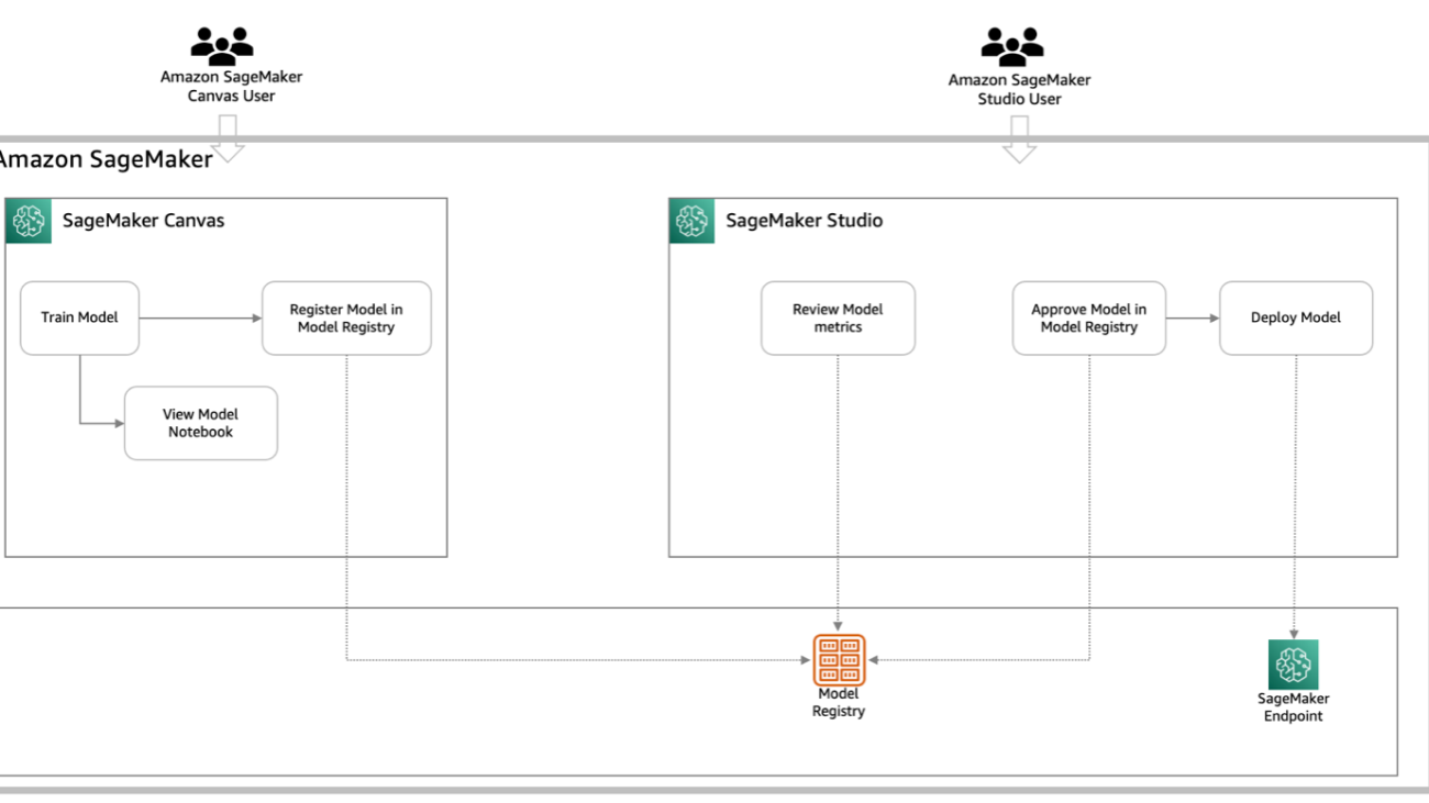
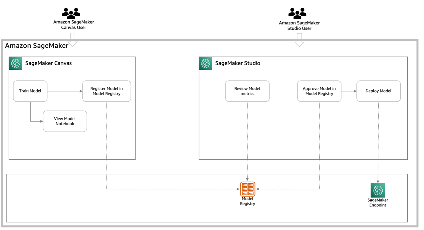
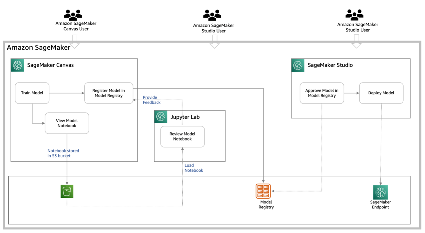
  • Option 1: SageMaker Model Registry – A SageMaker Canvas user registers their model in the Amazon SageMaker Model Registry, invoking a governance workflow for ML experts to review model details and metrics, then approve or reject it, after which the user can deploy the approved model from SageMaker Canvas. This option is an automated sharing process providing you with built-in governance and approval tracking. You can view the model metrics; however, there is limited visibility on the model code and architecture. The following diagram illustrates the architecture.

Option 1: SageMaker Model Registry

  • Option 2: Notebook export – In this option, the SageMaker Canvas user exports the full notebook from SageMaker Canvas to Amazon Simple Storage Service (Amazon S3), then shares it with ML experts to import into SageMaker Studio, enabling complete visibility and customization of the model code and logic before the ML expert deploys the enhanced model. In this option, there is complete visibility of the model code and architecture with the ability for the ML expert to customize and enhance the model in SageMaker Studio. However, this option demands a manual export and import of the model notebook into the IDE. The following diagram illustrates this architecture.

Option 2: Notebook export

The following phases describe the steps for collaboration:

  • Share – The SageMaker Canvas user registers the model from SageMaker Canvas or downloads the notebook from SageMaker Canvas
  • Review – The SageMaker Studio user accesses the model through the model registry to review and run the exported notebook through JupyterLab to validate the model
  • Approval – The SageMaker Studio user approves the model from the model registry
  • Deploy – The SageMaker Studio user can deploy the model from JupyterLab, or the SageMaker Canvas user can deploy the model from SageMaker Canvas

Let’s look at the two options (model registry and notebook export) within each step in detail.

Prerequisites

Before you dive into the solution, make sure you have signed up for and created an AWS account. Then you need to create an administrative user and a group. For instructions on both steps, refer to Set Up Amazon SageMaker Prerequisites. You can skip this step if you already have your own version of SageMaker Studio running.

Complete the prerequisites for setting up SageMaker Canvas and create the model of your choice for your use case.

Share the model

The SageMaker Canvas user shares the model with the SageMaker Studio user by either registering it in SageMaker Model Registry, which triggers a governance workflow, or by downloading the full notebook from SageMaker Canvas and providing it to the SageMaker Studio user.

SageMaker Model Registry

To deploy using SageMaker Model Registry, complete the following steps:

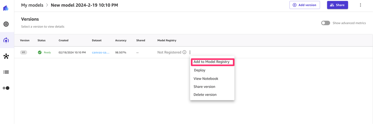
  1. After a model is created in SageMaker Canvas, choose the options menu (three vertical dots) and choose Add to Model Registry.
    add to model registry
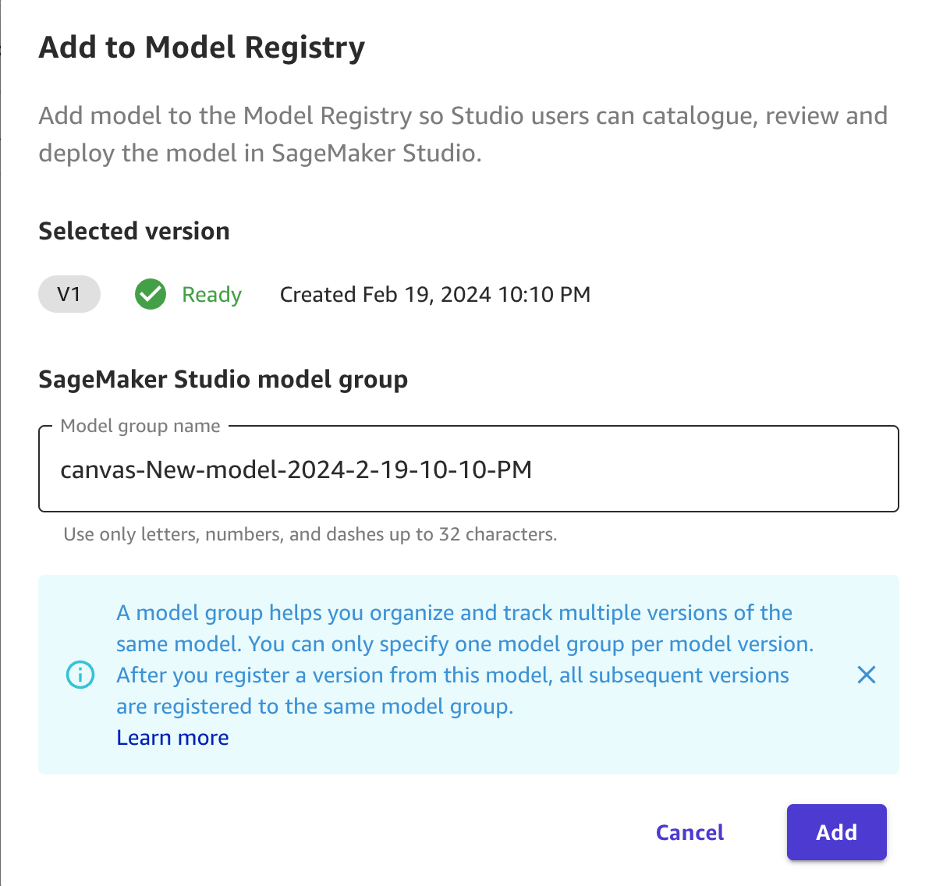
  2. Enter a name for the model group.
  3. Choose Add.
    model group name

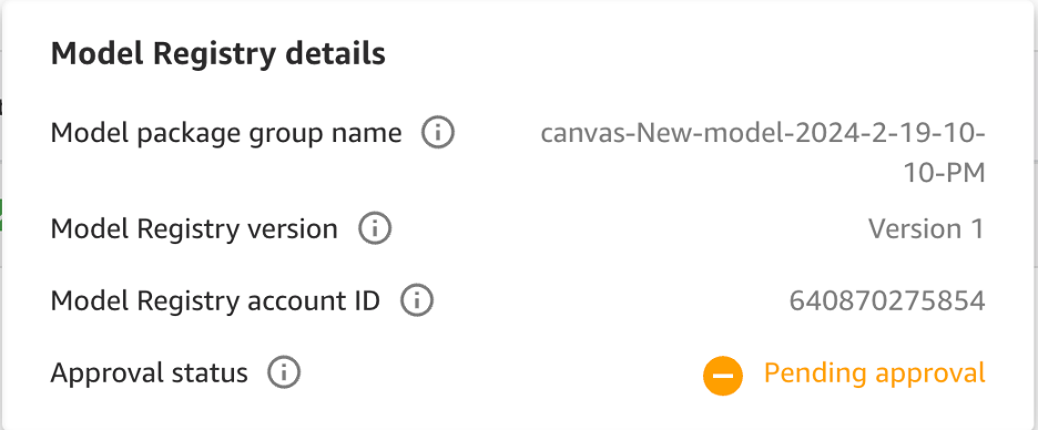
You can now see the model is registered.
model registered

You can also see the model is pending approval.
pending approval

SageMaker notebook export

To deploy using a SageMaker notebook, complete the following steps:

  1. On the options menu, choose View Notebook.
    view notebook
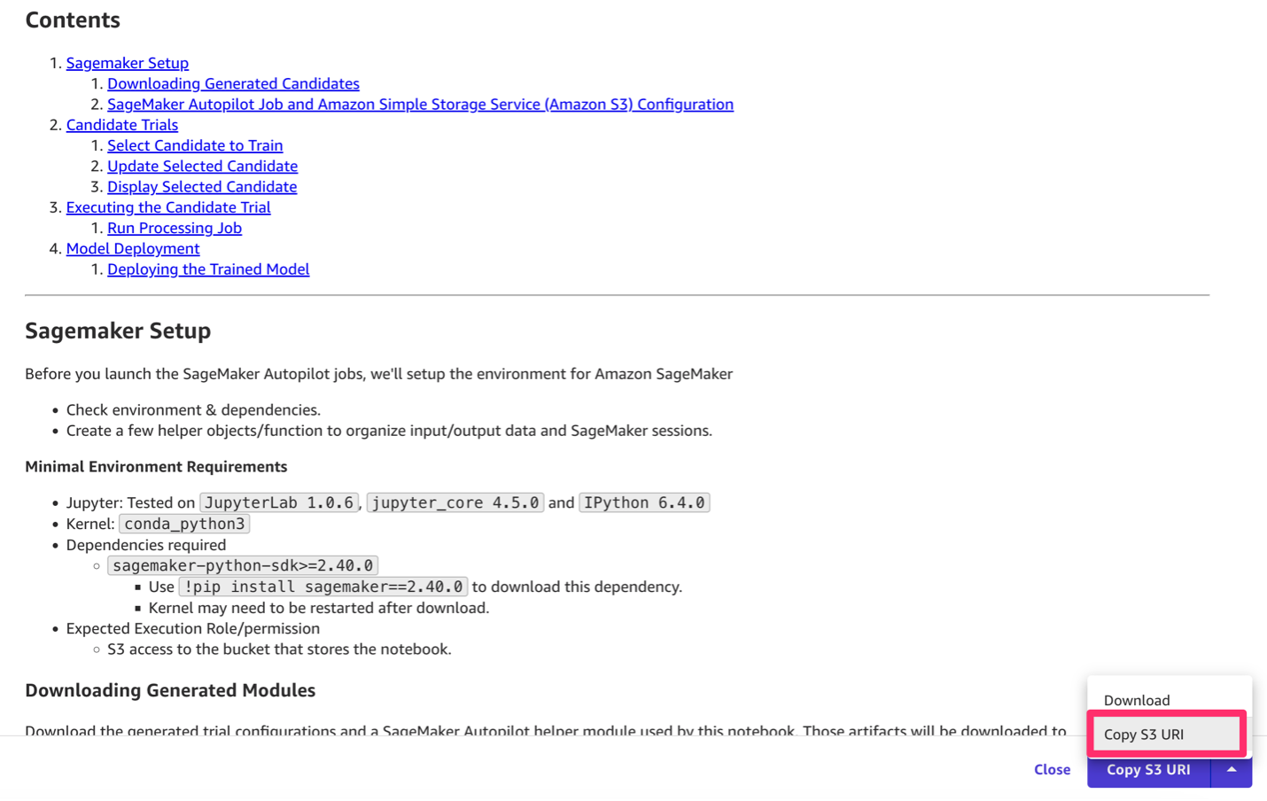
  2. Choose Copy S3 URI.
    s3 uri

You can now share the S3 URI with the SageMaker Studio user.

Review the model

The SageMaker Studio user accesses the shared model through the model registry to review its details and metrics, or they can import the exported notebook into SageMaker Studio and use Jupyter notebooks to thoroughly validate the model’s code, logic, and performance.

SageMaker Model Registry

To use the model registry, complete the following steps:

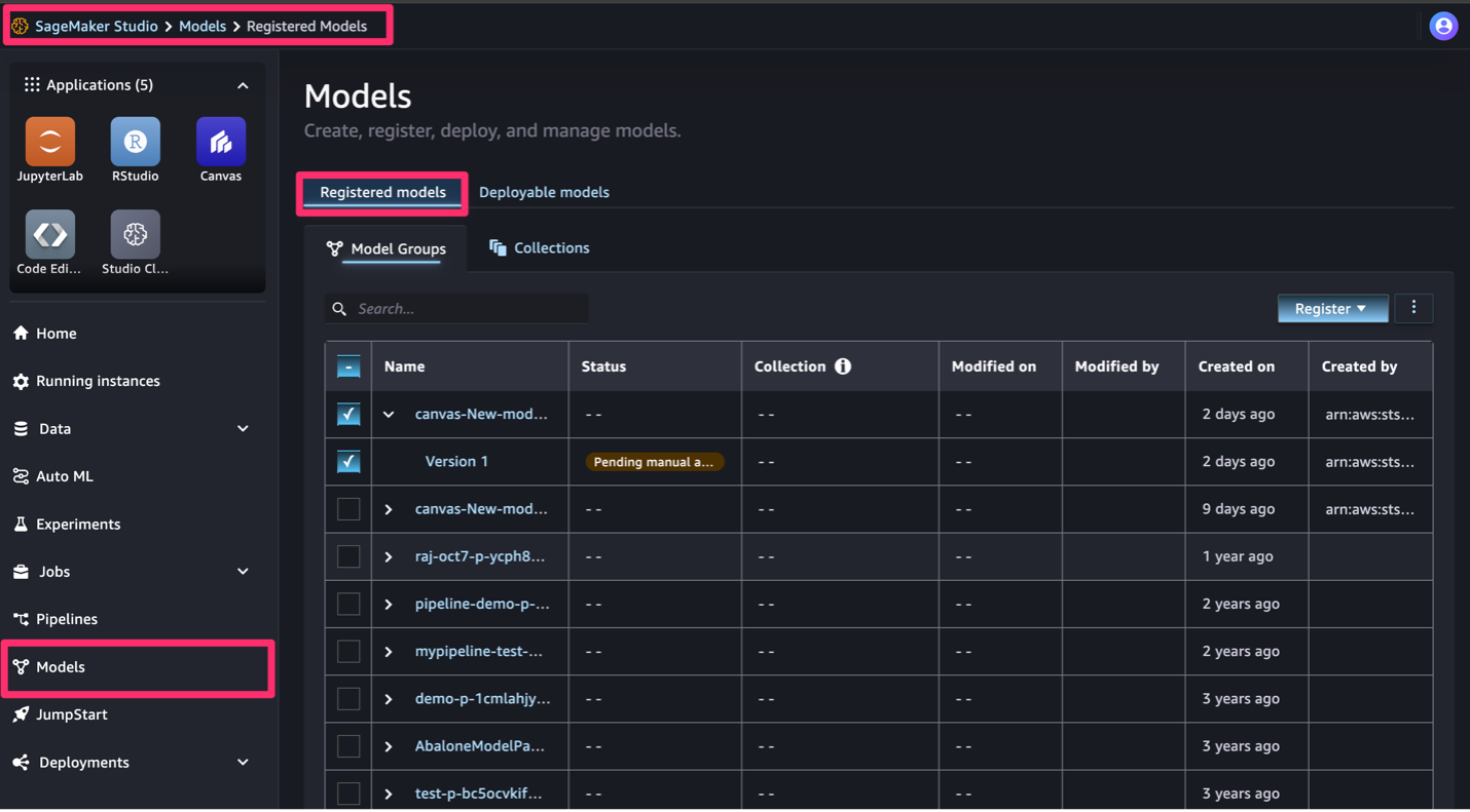
  1. On the SageMaker Studio console, choose Models in the navigation pane.
  2. Choose Registered models.
  3. Choose your model.
    model registry

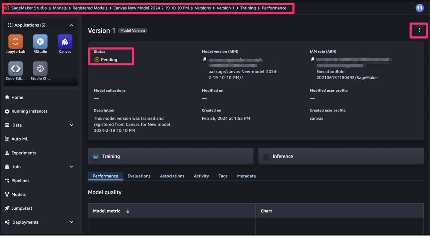
You can review the model details and see that the status is pending.
status pending

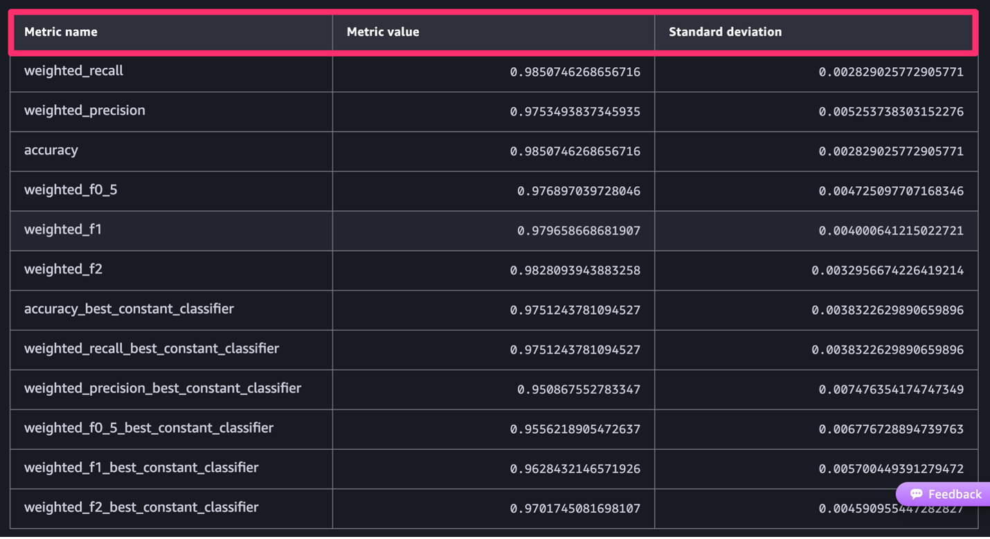
You can also review the different metrics to check on the model performance.
review metrics

You can view the model metrics; however, there is limited visibility on the model code and architecture. If you want complete visibility of the model code and architecture with the ability to customize and enhance the model, use the notebook export option.

SageMaker notebook export

To use the notebook export option as the SageMaker Studio user, complete the following steps.

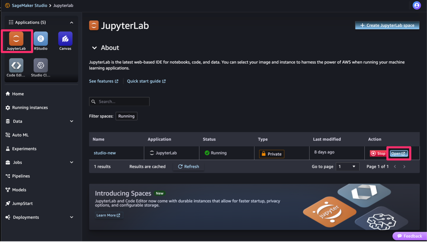
  1. Launch SageMaker Studio and choose JupyterLab under Applications.
  2. Open the JupyterLab space.If you don’t have a JupyterLab space, you can create one.
    jupyter lab
  3. Open a terminal and run the following command to copy the notebook from Amazon S3 to SageMaker Studio (the account number in the following example is changed to awsaccountnumber):
    sagemaker-user@default:~$ aws s3 cp s3://sagemaker-us-east-1-awsaccountnumber/Canvas/default-20240130t161835/Training/output/Canvas1707947728560/sagemaker-automl-candidates/notebooks/SageMakerAutopilotCandidateDefinitionNotebook.ipynb ./canvas.ipynb

    terminal

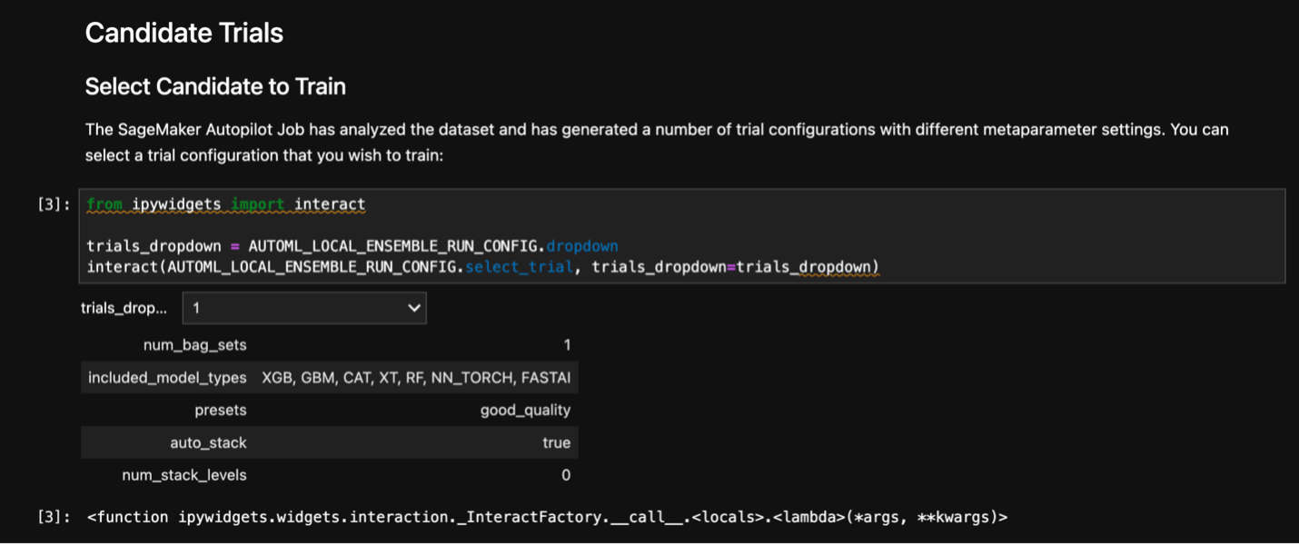
  4. After the notebook is downloaded, you can open the notebook and run the notebook to evaluate further.

candidate trials

Approve the model

After a comprehensive review, the SageMaker Studio user can make an informed decision to either approve or reject the model in the model registry based on their assessment of its quality, accuracy, and suitability for the intended use case.

For users who registered their model via the Canvas UI, please follow the below steps to approve the model. For users who exported the model notebook from the Canvas UI, you may register and approve the model using SageMaker model registry, however, these steps are not required.

SageMaker Model Registry

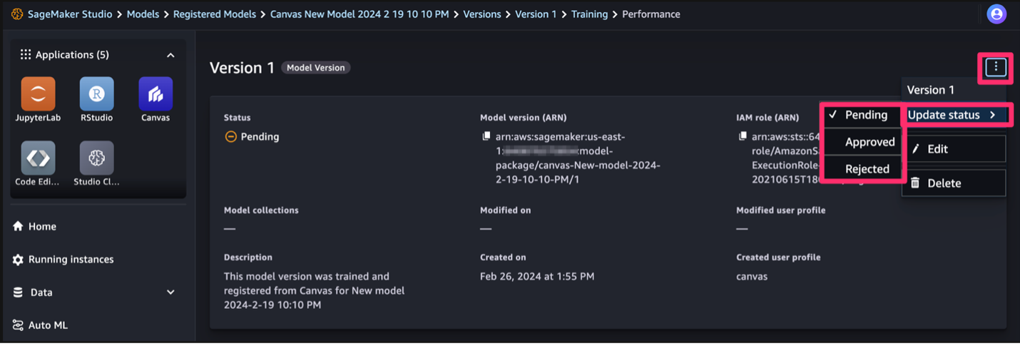
As the SageMaker Studio user, when you’re comfortable with the model, you can update the status to approved. Approval happens only in SageMaker Model Registry. Complete the following steps:

  1. In SageMaker Studio, navigate to the version of the model.
  2. On the options menu, choose Update status and Approved.
    status update
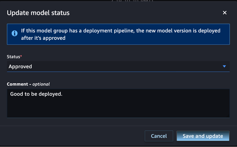
  3. Enter an optional comment and choose Save and update.
    update model status

Now you can see the model is approved.
approved

Deploy the model

Once the model is ready to deploy (it has received necessary reviews and approvals), users have two options. For users who took the model registry approach, they can deploy from either SageMaker Studio or from SageMaker Canvas. For users who took the model notebook export approach, they can deploy from SageMaker Studio. Both deployment options are detailed below.

Deploy via SageMaker Studio

The SageMaker Studio user can deploy the model from the JupyterLab space.
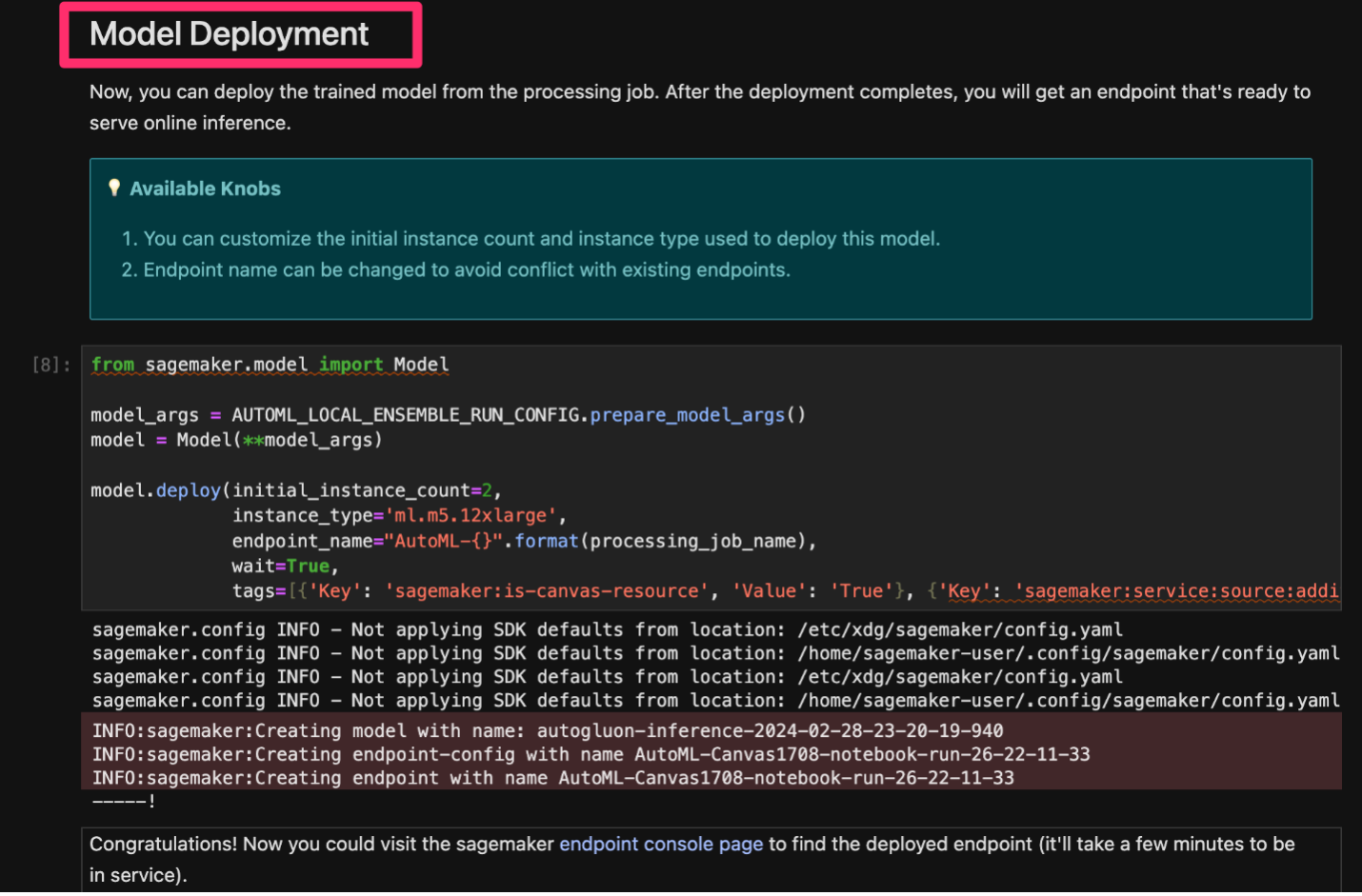
model deployment

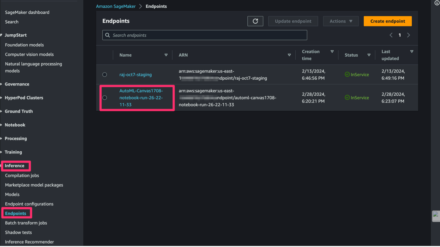
After the model is deployed, you can navigate to the SageMaker console, choose Endpoints under Inference in the navigation pane, and view the model.
endpoints

Deploy via SageMaker Canvas

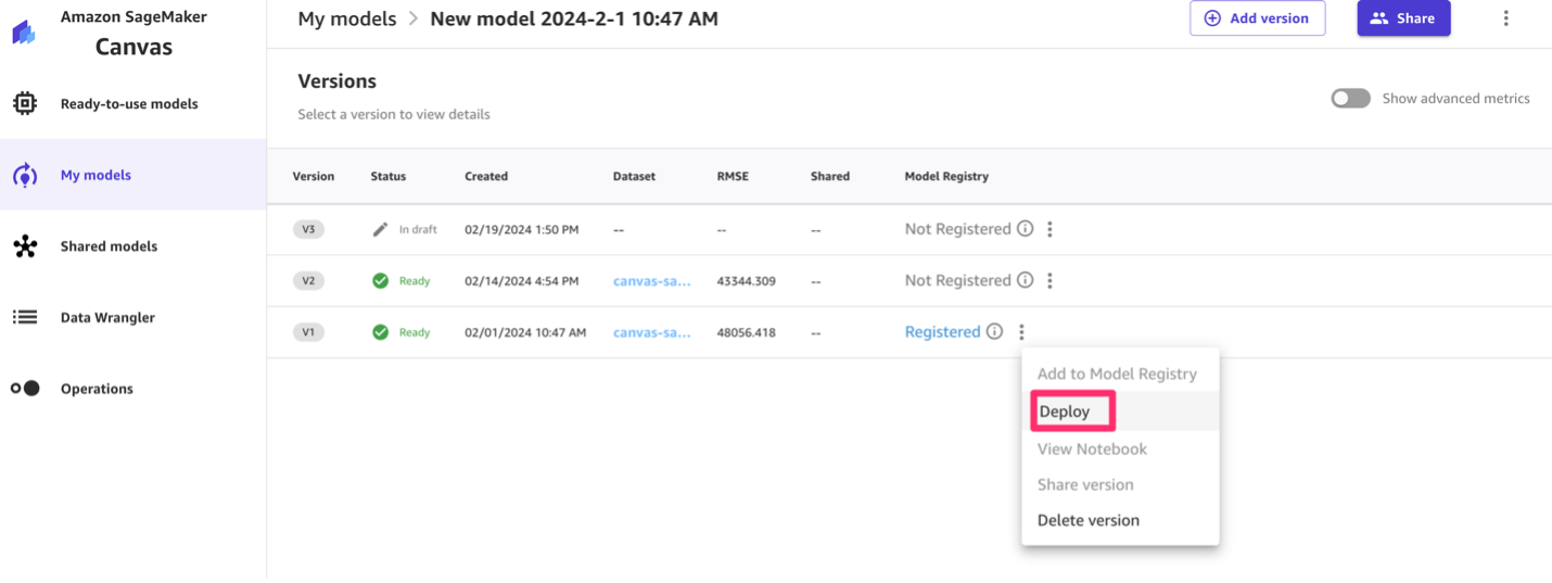
Alternatively, if the deployment is handled by the SageMaker Canvas user, you can deploy the model from SageMaker Canvas.

canvas deploy

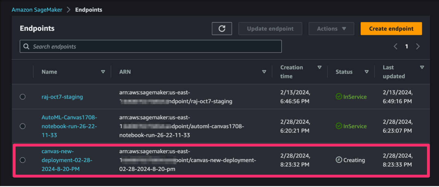
After the model is deployed, you can navigate to the Endpoints page on the SageMaker console to view the model.
deployed endpoints

Clean up

To avoid incurring future session charges, log out of SageMaker Canvas.

To avoid ongoing charges, delete the SageMaker inference endpoints. You can delete the endpoints via the SageMaker console or from the SageMaker Studio notebook using the following commands:

predictor.delete_model()

predictor.delete_endpoint()

Conclusion

Previously, you could only share models to SageMaker Canvas (or view shared SageMaker Canvas models) in SageMaker Studio Classic. In this post, we showed how to share models built in SageMaker Canvas with SageMaker Studio so that different teams can collaborate and you can pivot from a no-code to a high-code deployment path. By either using SageMaker Model Registry or exporting notebooks, ML experts and non-experts can collaborate, review, and enhance models across these platforms, enabling a smooth workflow from data preparation to production deployment.

For more information about collaborating on models using SageMaker Canvas, refer to Build, Share, Deploy: how business analysts and data scientists achieve faster time-to-market using no-code ML and Amazon SageMaker Canvas.


About the Authors

Rajakumar Sampathkumar is a Principal Technical Account Manager at AWS, providing customer guidance on business-technology alignment and supporting the reinvention of their cloud operation models and processes. He is passionate about cloud and machine learning. Raj is also a machine learning specialist and works with AWS customers to design, deploy, and manage their AWS workloads and architectures.

Meenakshisundaram Thandavarayan works for AWS as an AI/ ML Specialist. He has a passion to design, create, and promote human-centered data and analytics experiences. Meena focusses on developing sustainable systems that deliver measurable, competitive advantages for strategic customers of AWS. Meena is a connector and design thinker, and strives to drive business to new ways of working through innovation, incubation, and democratization.

Claire O’Brien Rajkumar is a Sr. Product Manager on the Amazon SageMaker team focused on SageMaker Canvas, the SageMaker low-code no-code workspace for ML and generative AI. SageMaker Canvas helps democratize ML and generative AI by lowering barriers to adoption for those new to ML and accelerating workflows for advanced practitioners.

Read More

Research Focus: Week of April 1, 2024

Research Focus: Week of April 1, 2024

Welcome to Research Focus, a series of blog posts that highlights notable publications, events, code/datasets, new hires and other milestones from across the research community at Microsoft.

Research Focus April 1, 2024

LLMs in the Imaginarium: Tool Learning through Simulated Trial and Error

In the same way that tools can help people complete tasks beyond their innate abilities, tools are essential for large language models (LLMs) to acquire up-to-date information and take consequential actions in external environments. Existing work on tool-augmented LLMs primarily focuses on the broad coverage of tools and the flexibility of adding new tools. However, a surprisingly understudied question is how accurately an LLM uses tools for which it has been trained.

In a recent paper: LLMs in the Imaginarium: Tool Learning through Simulated Trial and Error, researchers from Microsoft find that existing LLMs, including GPT-4 and open-source LLMs specifically fine-tuned for tool use, only reach a correctness rate of 30% to 60%, which is too unreliable for practical use. They propose a biologically inspired method for tool-augmented LLMs – simulated trial and error (STE) – that orchestrates three key mechanisms: trial and error, imagination, and memory. STE simulates plausible scenarios for using a tool, then the LLM interacts with the tool to learn from its execution feedback. Both short-term and long-term memory are employed to improve the depth and breadth of the exploration. Experiments on ToolBench show STE substantially improves tool learning for LLMs under both in-context learning and fine-tuning settings.

Microsoft Research Podcast

AI Frontiers: AI for health and the future of research with Peter Lee

Peter Lee, head of Microsoft Research, and Ashley Llorens, AI scientist and engineer, discuss the future of AI research and the potential for GPT-4 as a medical copilot.


Benchmarking Large Language Models Across Languages, Modalities, Models and Tasks

The latest LLMs have surpassed the performance of older language models on several tasks and benchmarks, sometimes approaching or even exceeding human performance. Yet, it is not always clear whether this is due to the increased capabilities of these models, or other effects, such as artifacts in datasets, test dataset contamination, and the lack of datasets that measure the true capabilities of these models.

As a result, research to comprehend LLM capabilities and limitations has surged of late. However, much of this research has been confined to English, leaving LLM building and evaluation for non-English languages relatively unexplored. Several new LLMs have been introduced recently, necessitating their evaluation on non-English languages. In a recent paper: MEGAVERSE: Benchmarking Large Language Models Across Languages, Modalities, Models and Tasks, researchers from Microsoft aim to perform a thorough evaluation of the non-English capabilities of state-of-the-art LLMs (GPT-3.5-Turbo, GPT-4, PaLM2, Mistral, Gemini, Gemma and Llama2) by comparing them on the same set of multilingual datasets. Their benchmark comprises 22 datasets covering 81 languages including several low-resource African languages. They also include two multimodal datasets in the benchmark and compare the performance of LLaVA-v1.5 and GPT-4-Vision. Experiments show that GPT-4 and PaLM2 outperform the Llama and Mistral models on various tasks, notably on low-resource languages, with GPT-4 outperforming PaLM2 on more datasets. However, issues such as data contamination must be addressed to obtain an accurate assessment of LLM performance on non-English languages.


Training Audio Captioning Models without Audio

Automated Audio Captioning (AAC) is a process that creates text descriptions for audio recordings. Unlike Closed Captioning, which transcribes speech, AAC aims to describe all sounds in the audio (e.g. : A muffled rumble with people talking in the background while a siren blares in the distance). Typical AAC systems require expensive curated data of audio-text pairs, which often results in a shortage of suitable data, impeding model training.

In this paper: Training Audio Captioning Models without Audio, researchers from Microsoft and Carnegie Mellon University propose a new paradigm for training AAC systems, using text descriptions alone, thereby eliminating the requirement for paired audio and text descriptions. Their approach leverages CLAP, a contrastive learning model that uses audio and text encoders to create a shared vector representation between audio and text. For instance, the text “siren blaring” and its corresponding audio recording would share the same vector. The model is trained on text captions: a GPT language decoder generates captions conditioned on the pretrained CLAP text encoder and a mapping network. During inference, audio input is first converted to its vector using the pretrained CLAP audio encoder and then a text caption is generated.

The researchers find that the proposed text-only framework competes well with top-tier models trained on both text and audio, proving that efficient text-to-audio conversion is possible. They also demonstrated the ability to incorporate various writing styles, such as humorous, beneficial for tailoring caption generation to specific fields. Finally, they highlight that enriching training with LLM-generated text leads to improved performance and has potential in increasing vocabulary diversity.

The post Research Focus: Week of April 1, 2024 appeared first on Microsoft Research.

Read More