Monthly Archives: June 2024

Amazon SageMaker JumpStart is a machine learning (ML) hub offering pre-trained models and pre-built solutions. It provides access to hundreds of foundation models (FMs). A private hub is a feature in SageMaker JumpStart that allows an organization to share their models and notebooks so as to centralize model artifacts, facilitate discoverability, and increase the reuse within the organization. With new models released daily, many enterprise admins want more control over the FMs that can be discovered and used by users within their organization (for example, only allowing models based on pytorch framework to be discovered).

Now enterprise admins can effortlessly configure granular access control over the FMs that SageMaker JumpStart provides out of box so that only allowed models can be accessed by users within their organizations. In this post, we discuss the steps required for an administrator to configure granular access control of models in SageMaker JumpStart using a private hub, as well as the steps for users to access and consume models from the private hub.

Solution overview

Starting today, with SageMaker JumpStart and its private hub feature, administrators can create repositories for a subset of models tailored to different teams, use cases, or license requirements using the Amazon SageMaker Python SDK. Admins can also set up multiple private hubs with different lists of models discoverable for different groups of users. Users are then only able to discover and use models within the private hubs they have access to through Amazon SageMaker Studio and the SDK. This level of control empowers enterprises to consume the latest in open weight generative artificial intelligence (AI) development while enforcing governance guardrails. Finally, admins can share access to private hubs across multiple AWS accounts, enabling collaborative model management while maintaining centralized control. SageMaker JumpStart uses AWS Resource Access Manager (AWS RAM) to securely share private hubs with other accounts in the same organization. The new feature is available in the us-east-2 AWS Region as of writing, and will be available to more Regions soon.

The following diagram shows an example architecture of SageMaker JumpStart with its public and private hub features. The diagram illustrates how SageMaker JumpStart provides access to different model repositories, with some users accessing the public SageMaker JumpStart hub and others using private curated hubs.

In the following section, we demonstrate how admins can configure granular access control of models in SageMaker JumpStart using a private hub. Then we show how users can access and consume allowlisted models in the private hub using SageMaker Studio and the SageMaker Python SDK. Finally, we look at how an admin user can share the private hub with users in another account.

Prerequisites

To use the SageMaker Python SDK and run the code associated with this post, you need the following prerequisites:

• An AWS account that contains all your AWS resources
• An AWS Identity and Access Management (IAM) role with access to SageMaker Studio notebooks
• SageMaker JumpStart enabled in a SageMaker Studio domain

Create a private hub, curate models, and configure access control (admins)

This section provides a step-by-step guide for administrators to create a private hub, curate models, and configure access control for your organization’s users.

1. Because the feature has been integrated in the latest SageMaker Python SDK, to use the model granular access control feature with a private hub, let’s first update the SageMaker Python SDK:

   !pip3 install sagemaker —force-reinstall —quiet

2. Next, import the SageMaker and Boto3 libraries:

   import boto3
   from sagemaker import Session
   from sagemaker.jumpstart.hub.hub import Hub

3. Configure your private hub:

   HUB_NAME="CompanyHub"
   HUB_DISPLAY_NAME="Allowlisted Models"
   HUB_DESCRIPTION="These are allowlisted models taken from the JumpStart Public Hub."
   REGION="<your_region_name>" # for example, "us-west-2"

   In the preceding code, HUB_NAME specifies the name of your Hub. HUB_DISPLAY_NAME is the display name for your hub that will be shown to users in UI experiences. HUB_DESCRIPTION is the description for your hub that will be shown to users.

4. Set up a Boto3 client for SageMaker:

   sm_client = boto3.client('sagemaker')
   session = Session(sagemaker_client=sm_client)
   session.get_caller_identity_arn()

5. Check if the following policies have been already added to your admin IAM role; if not, you can add them as inline policies:

   {
       "Version": "2012-10-17",
       "Statement": [
           {
               "Action": [
                   "s3:ListBucket",
                   "s3:GetObject",
                   "s3:GetObjectTagging"
               ],
               "Resource": [
                   "arn:aws:s3:::jumpstart-cache-prod-<REGION>",
                   "arn:aws:s3:::jumpstart-cache-prod-<REGION>/*"
               ],
               "Effect": "Allow"
           }
       ]
   }

   Replace the <REGION> placeholder using the configurations in Step 3.

   In addition to setting up IAM permissions to the admin role, you need to scope down permissions for your users so they can’t access public contents.

6. Use the following policy to deny access to the public hub for your users. These can be added as inline policies in the user’s IAM role:

   {
       "Version": "2012-10-17",
       "Statement": [
           {
               "Action": "s3:*",
               "Effect": "Deny",
               "Resource": [
                   "arn:aws:s3:::jumpstart-cache-prod-<REGION>",
                   "arn:aws:s3:::jumpstart-cache-prod-<REGION>/*"
               ],
               "Condition": {
                   "StringNotLike": {"s3:prefix": ["*.ipynb", "*/eula.txt"]}
               }
           },
           {
               "Action": "sagemaker:*",
               "Effect": "Deny",
               "Resource": [
                   "arn:aws:sagemaker:<REGION>:aws:hub/SageMakerPublicHub",
                   "arn:aws:sagemaker:<REGION>:aws:hub-content/SageMakerPublicHub/*/*"
               ]
           }
       ]
   }
   

   Replace the <REGION> placeholder in the policy using the configurations in Step 3.

   After you have set up the private hub configuration and permissions, you’re ready to create the private hub.

7. Use the following code to create the private hub within your AWS account in the Region you specified earlier:

   hub = Hub(hub_name=HUB_NAME, sagemaker_session=session)
   
   try:
     hub.create(
         description=HUB_DESCRIPTION,
         display_name=HUB_DISPLAY_NAME
     )
     print(f"Successfully created Hub with name {HUB_NAME} in {REGION}")
   except Exception as e:
     if "ResourceInUse" in str(e):
       print(f"A hub with the name {HUB_NAME} already exists in your account.")
     else:
       raise e
   

8. Use hub.describe() to verify the configuration of your hub.After your private hub is set up, you can add a reference to models from the SageMaker JumpStart public hub to your private hub. No model artifacts need to be managed by the customer. The SageMaker team will manage any version or security updates.For a list of available models, refer to Built-in Algorithms with pre-trained Model Table.
9. To search programmatically, run the command

   filter_value = "framework == meta"
   response = hub.list_sagemaker_public_hub_models(filter=filter_value)
   models = response["hub_content_summaries"]
   while response["next_token"]:
       response = hub.list_sagemaker_public_hub_models(filter=filter_value,
                                                       next_token=response["next_token"])
       models.extend(response["hub_content_summaries"])
   
   print(models)
   

   The filter argument is optional. For a list of filters you can apply, refer to SageMaker Python SDK.

10. Use the retrieved models from the preceding command to create model references for your private hub:

    for model in models:
        print(f"Adding {model.get('hub_content_name')} to Hub")
        hub.create_model_reference(model_arn=model.get("hub_content_arn"), 
                                   model_name=model.get("hub_content_name"))

    The SageMaker JumpStart private hub offers other useful features for managing and interacting with the curated models. Administrators can check the metadata of a specific model using the hub.describe_model(model_name=<model_name>) command. To list all available models in the private hub, you can use a simple loop:

    response = hub.list_models()
    models = response["hub_content_summaries"]
    while response["next_token"]:
        response = hub.list_models(next_token=response["next_token"])
        models.extend(response["hub_content_summaries"])
    
    for model in models:
        print(model.get('HubContentArn'))
    

    If you need to remove a specific model reference from the private hub, use the following command:

    hub.delete_model_reference("<model_name>")

    If you want to delete the private hub from your account and Region, you’ll need to delete all the HubContents first, then delete the private hub. Use the following code:

    for model in models:
        hub.delete_model_reference(model_name=model.get('HubContentName')) 
    
    hub.delete()
    

Interact with allowlisted models (users)

This section offers a step-by-step guide for users to interact with allowlisted models in SageMaker JumpStart. We demonstrate how to list available models, identify a model from the public hub, and deploy the model to endpoints from SageMaker Studio as well as the SageMaker Python SDK.

User experience in SageMaker Studio

Complete the following steps to interact with allowlisted models using SageMaker Studio:

1.  On the SageMaker Studio console, choose JumpStart in the navigation pane or in the Prebuilt and automated solutions section.
2. Choose one of model hubs you have access to. If the user has access to multiple hubs, you’ll see a list of hubs, as shown in the following screenshot.
   If the user has access to only one hub, you’ll go straight to the model list.
   You can view the model details and supported actions like train, deploy, and evaluate.
3. To deploy a model, choose Deploy.
4. Modify your model configurations like instances and deployment parameters, and choose Deploy.

User experience using the SageMaker Python SDK

To interact with your models using the SageMaker Python SDK, complete the following steps:

1. Just like the admin process, the first step is to force reinstall the SageMaker Python SDK:

   !pip3 install sagemaker —force-reinstall —quiet

2. Import the SageMaker and Boto3 libraries:

   import boto3
   from sagemaker import Session
   from sagemaker.jumpstart.hub.hub import Hub
   from sagemaker.jumpstart.model import JumpStartModel
   from sagemaker.jumpstart.estimator import JumpStartEstimator

3. To access the models in your private hub, you need the Region and the name of the hub on your account. Fill out the HUB_NAME and REGION fields with the information provided by your administrator:

   HUB_NAME="CompanyHub" 
   REGION="<your_region_name>" # for example, "us-west-2"
   sm_client = boto3.client('sagemaker') 
   sm_runtime_client = boto3.client('sagemaker-runtime') 
   session = Session(sagemaker_client=sm_client, 
                       sagemaker_runtime_client=sm_runtime_client)
   hub = Hub(hub_name=HUB_NAME, sagemaker_session=session)

4. List the models available in your private hub using the following command:

   response = hub.list_models()
   models = response["hub_content_summaries"]
   while response["next_token"]:
       response = hub.list_models(next_token=response["next_token"])
       models.extend(response["hub_content_summaries"])
   
   print(models)

5. To get more information about a particular model, use the describe_model method:

   model_name = "huggingface-llm-phi-2"
   response = hub.describe_model(model_name=model_name) 
   print(response)

6. You can deploy models in a hub with the Python SDK by using JumpStartModel. To deploy a model from the hub to an endpoint and invoke the endpoint with the default payloads, run the following code. To select which model from your hub you want to use, pass in a model_id and version. If you pass in * for the version, it will take the latest version available for that model_id in the hub. If you’re using a model gated behind a EULA agreement, pass in accept_eula=True.

   model_id, version = "huggingface-llm-phi-2", "1.0.0"
   model = JumpStartModel(model_id, version, hub_name=HUB_NAME, 
                               region=REGION, sagemaker_session=session)
   predictor = model.deploy(accept_eula=False)

7. To invoke your deployed model with the default payloads, use the following code:

   example_payloads = model.retrieve_all_examples()
   for payload in example_payloads:
       response = predictor.predict(payload.body)
       print("nInputn", payload.body, "nnOutputn", 
                   response[0]["generated_text"], "nn===============")

8. To delete the model endpoints that you created, use the following code:

   predictor.delete_model()
   predictor.delete_endpoint()

Cross-account sharing of private hubs

SageMaker JumpStart private hubs support cross-account sharing, allowing you to extend the benefits of your curated model repository beyond your own AWS account. This feature enables collaboration across different teams or departments within your organization, even when they operate in separate AWS accounts. By using AWS RAM, you can securely share your private hubs while maintaining control over access.

To share your private hub across accounts, complete the following steps:

1. On the AWS RAM console, choose Create resource share.
2. When specifying resource share details, choose the SageMaker hub resource type and select one or more private hubs that you want to share. When you share a hub with any other account, all of its contents are also shared implicitly.
3. Associate permissions with your resource share.
4. Use AWS account IDs to specify the accounts to which you want to grant access to your shared resources.
5. Review your resource share configuration and choose Create resource share.

It may take a few minutes for the resource share and principal associations to complete.

Admins that want to perform the preceding steps programmatically can enter the following command to initiate the sharing:

# create a resource share using the private hub
aws ram create-resource-share 
    --name test-share 
    --resource-arns arn:aws:sagemaker:<region>:<resource_owner_account_id>:hub/<hub_name> 
    --principals <consumer_account_id>  
    --region <region>

Replace the <resource_owner_account_id>, <consumer_account_id>, <hub_name>, and <region> placeholders with the appropriate values for the resource owner account ID, consumer account ID, name of the hub, and Region to use.

After you set up the resource share, the specified AWS account will receive an invitation to join. They must accept this invitation through AWS RAM to gain access to the shared private hub. This process makes sure access is granted only with explicit consent from both the hub owner and the recipient account. For more information, refer to Using shared AWS resources.

You can also perform this step programmatically:

# list resource shares
aws ram get-resource-share-invitations 
    --region <region>

# accept resource share
# using the arn from the previous response 
aws ram accept-resource-share-invitation  
  --resource-share-invitation-arn <arn_from_ previous_request> 
  --region <region>

For detailed instructions on creating resource shares and accepting invitations, refer to Creating a resource share in AWS RAM. By extending your private hub across accounts, you can foster collaboration and maintain consistent model governance across your entire organization.

Conclusion

SageMaker JumpStart allows enterprises to adopt FMs while maintaining granular control over model access and usage. By creating a curated repository of approved models in private hubs, organizations can align their AI initiatives with corporate policies and regulatory requirements. The private hub decouples model curation from model consumption, enabling administrators to manage the model inventory while data scientists focus on developing AI solutions.

This post explained the private hub feature in SageMaker JumpStart and provided steps to set up and use a private hub, with minimal additional configuration required. Administrators can select models from the public SageMaker JumpStart hub, add them to the private hub, and manage user access through IAM policies. Users can then deploy these preapproved models, fine-tune them on custom datasets, and integrate them into their applications using familiar SageMaker interfaces. The private hub uses the SageMaker underlying infrastructure, allowing it to scale with enterprise-level ML demands.

For more information about SageMaker JumpStart, refer to SageMaker JumpStart. To get started using SageMaker JumpStart, access it through SageMaker Studio.

About the Authors

Raju Rangan is a Senior Solutions Architect at AWS. He works with government-sponsored entities, helping them build AI/ML solutions using AWS. When not tinkering with cloud solutions, you’ll catch him hanging out with family or smashing birdies in a lively game of badminton with friends.

Sherry Ding is a senior AI/ML specialist solutions architect at AWS. She has extensive experience in machine learning with a PhD in computer science. She mainly works with public sector customers on various AI/ML-related business challenges, helping them accelerate their machine learning journey on the AWS Cloud. When not helping customers, she enjoys outdoor activities.

June Won is a product manager with Amazon SageMaker JumpStart. He focuses on making foundation models easily discoverable and usable to help customers build generative AI applications. His experience at Amazon also includes mobile shopping applications and last mile delivery.

Bhaskar Pratap is a Senior Software Engineer with the Amazon SageMaker team. He is passionate about designing and building elegant systems that bring machine learning to people’s fingertips. Additionally, he has extensive experience with building scalable cloud storage services.

Read More

eSentire is an industry-leading provider of Managed Detection & Response (MDR) services protecting users, data, and applications of over 2,000 organizations globally across more than 35 industries. These security services help their customers anticipate, withstand, and recover from sophisticated cyber threats, prevent disruption from malicious attacks, and improve their security posture.

In 2023, eSentire was looking for ways to deliver differentiated customer experiences by continuing to improve the quality of its security investigations and customer communications. To accomplish this, eSentire built AI Investigator, a natural language query tool for their customers to access security platform data by using AWS generative artificial intelligence (AI) capabilities.

In this post, we share how eSentire built AI Investigator using Amazon SageMaker to provide private and secure generative AI interactions to their customers.

Benefits of AI Investigator

Before AI Investigator, customers would engage eSentire’s Security Operation Center (SOC) analysts to understand and further investigate their asset data and associated threat cases. This involved manual effort for customers and eSentire analysts, forming questions and searching through data across multiple tools to formulate answers.

eSentire’s AI Investigator enables users to complete complex queries using natural language by joining multiple sources of data from each customer’s own security telemetry and eSentire’s asset, vulnerability, and threat data mesh. This helps customers quickly and seamlessly explore their security data and accelerate internal investigations.

Providing AI Investigator internally to the eSentire SOC workbench has also accelerated eSentire’s investigation process by improving the scale and efficacy of multi-telemetry investigations. The LLM models augment SOC investigations with knowledge from eSentire’s security experts and security data, enabling higher-quality investigation outcomes while also reducing time to investigate. Over 100 SOC analysts are now using AI Investigator models to analyze security data and provide rapid investigation conclusions.

Solution overview

eSentire customers expect rigorous security and privacy controls for their sensitive data, which requires an architecture that doesn’t share data with external large language model (LLM) providers. Therefore, eSentire decided to build their own LLM using Llama 1 and Llama 2 foundational models. A foundation model (FM) is an LLM that has undergone unsupervised pre-training on a corpus of text. eSentire tried multiple FMs available in AWS for their proof of concept; however, the straightforward access to Meta’s Llama 2 FM through Hugging Face in SageMaker for training and inference (and their licensing structure) made Llama 2 an obvious choice.

eSentire has over 2 TB of signal data stored in their Amazon Simple Storage Service (Amazon S3) data lake. eSentire used gigabytes of additional human investigation metadata to perform supervised fine-tuning on Llama 2. This further step updates the FM by training with data labeled by security experts (such as Q&A pairs and investigation conclusions).

eSentire used SageMaker on several levels, ultimately facilitating their end-to-end process:

• They used SageMaker notebook instances extensively to spin up GPU instances, giving them the flexibility to swap high-power compute in and out when needed. eSentire used instances with CPU for data preprocessing and post-inference analysis and GPU for the actual model (LLM) training.
• The additional benefit of SageMaker notebook instances is its streamlined integration with eSentire’s AWS environment. Because they have vast amounts of data (terabyte scale, over 1 billion total rows of relevant data in preprocessing input) stored across AWS—in Amazon S3 and Amazon Relational Database Service (Amazon RDS) for PostgreSQL clusters—SageMaker notebook instances allowed secure movement of this volume of data directly from the AWS source (Amazon S3 or Amazon RDS) to the SageMaker notebook. They needed no additional infrastructure for data integration.
• SageMaker real-time inference endpoints provide the infrastructure needed for hosting their custom self-trained LLMs. This was very useful in combination with SageMaker integration with Amazon Elastic Container Registry (Amazon ECR), SageMaker endpoint configuration, and SageMaker models to provide the entire configuration required to spin up their LLMs as needed. The fully featured end-to-end deployment capability provided by SageMaker allowed eSentire to effortlessly and consistently update their model registry as they iterate and update their LLMs. All of this was entirely automated with the software development lifecycle (SDLC) using Terraform and GitHub, which is only possible through SageMaker ecosystem.

The following diagram visualizes the architecture diagram and workflow.

The application’s frontend is accessible through Amazon API Gateway, using both edge and private gateways. To emulate intricate thought processes akin to those of a human investigator, eSentire engineered a system of chained agent actions. This system uses AWS Lambda and Amazon DynamoDB to orchestrate a series of LLM invocations. Each LLM call builds upon the previous one, creating a cascade of interactions that collectively produce high-quality responses. This intricate setup makes sure that the application’s backend data sources are seamlessly integrated, thereby providing tailored responses to customer inquiries.

When a SageMaker endpoint is constructed, an S3 URI to the bucket containing the model artifact and Docker image is shared using Amazon ECR.

For their proof of concept, eSentire selected the Nvidia A10G Tensor Core GPU housed in an MLG5 2XL instance for its balance of performance and cost. For LLMs with significantly larger numbers of parameters, which demand greater computational power for both training and inference tasks, eSentire used 12XL instances equipped with four GPUs. This was necessary because the computational complexity and the amount of memory required for LLMs can increase exponentially with the number of parameters. eSentire plans to harness P4 and P5 instance types for scaling their production workloads.

Additionally, a monitoring framework that captures the inputs and outputs of AI Investigator was necessary to enable threat hunting visibility to LLM interactions. To accomplish this, the application integrates with an open sourced eSentire LLM Gateway project to monitor the interactions with customer queries, backend agent actions, and application responses. This framework enables confidence in complex LLM applications by providing a security monitoring layer to detect malicious poisoning and injection attacks while also providing governance and support for compliance through logging of user activity. The LLM gateway can also be integrated with other LLM services, such as Amazon Bedrock.

Amazon Bedrock enables you to customize FMs privately and interactively, without the need for coding. Initially, eSentire’s focus was on training bespoke models using SageMaker. As their strategy evolved, they began to explore a broader array of FMs, evaluating their in-house trained models against those provided by Amazon Bedrock. Amazon Bedrock offers a practical environment for benchmarking and a cost-effective solution for managing workloads due to its serverless operation. This serves eSentire well, especially when customer queries are sporadic, making serverless an economical alternative to persistently running SageMaker instances.

From a security perspective as well, Amazon Bedrock doesn’t share users’ inputs and model outputs with any model providers. Additionally, eSentire have custom guardrails for NL2SQL applied to their models.

Results

The following screenshot shows an example of eSentire’s AI Investigator output. As illustrated, a natural language query is posed to the application. The tool is able to correlate multiple datasets and present a response.

Dustin Hillard, CTO of eSentire, shares: “eSentire customers and analysts ask hundreds of security data exploration questions per month, which typically take hours to complete. AI Investigator is now with an initial rollout to over 100 customers and more than 100 SOC analysts, providing a self-serve immediate response to complex questions about their security data. eSentire LLM models are saving thousands of hours of customer and analyst time.”

Conclusion

In this post, we shared how eSentire built AI Investigator, a generative AI solution that provides private and secure self-serve customer interactions. Customers can get near real-time answers to complex questions about their data. AI Investigator has also saved eSentire significant analyst time.

The aforementioned LLM gateway project is eSentire’s own product and AWS bears no responsibility.

If you have any comments or questions, share them in the comments section.

About the Authors

Aishwarya Subramaniam is a Sr. Solutions Architect in AWS. She works with commercial customers and AWS partners to accelerate customers’ business outcomes by providing expertise in analytics and AWS services.

Ilia Zenkov is a Senior AI Developer specializing in generative AI at eSentire. He focuses on advancing cybersecurity with expertise in machine learning and data engineering. His background includes pivotal roles in developing ML-driven cybersecurity and drug discovery platforms.

Dustin Hillard is responsible for leading product development and technology innovation, systems teams, and corporate IT at eSentire. He has deep ML experience in speech recognition, translation, natural language processing, and advertising, and has published over 30 papers in these areas.

Read More

This is a guest post co-written with Ori Nakar from Imperva.

Imperva Cloud WAF protects hundreds of thousands of websites against cyber threats and blocks billions of security events every day. Counters and insights based on security events are calculated daily and used by users from multiple departments. Millions of counters are added daily, together with 20 million insights updated daily to spot threat patterns.

Our goal was to improve the user experience of an existing application used to explore the counters and insights data. The data is stored in a data lake and retrieved by SQL using Amazon Athena.

As part of our solution, we replaced multiple search fields with a single free text field. We used a large language model (LLM) with query examples to make the search work using the language used by Imperva internal users (business analysts).

The following figure shows a search query that was translated to SQL and run. The results were later formatted as a chart by the application. We have many types of insights—global, industry, and customer level insights used by multiple departments such as marketing, support, and research. Data was made available to our users through a simplified user experience powered by an LLM.

Figure 1: Insights search by natural language

Amazon Bedrock is a fully managed service that offers a choice of high-performing foundation models (FMs) from leading artificial intelligence (AI) companies such as AI21 Labs, Anthropic, Cohere, Meta, Mistral, Stability AI, and Amazon within a single API, along with a broad set of capabilities you need to build generative AI applications with security, privacy, and responsible AI. Amazon Bedrock Studio is a new single sign-on (SSO)-enabled web interface that provides a way for developers across an organization to experiment with LLMs and other FMs, collaborate on projects, and iterate on generative AI applications. It offers a rapid prototyping environment and streamlines access to multiple FMs and developer tools in Amazon Bedrock.

Read more to learn about the problem, and how we obtained quality results using Amazon Bedrock for our experimentation and deployment.

The problem

Making data accessible to users through applications has always been a challenge. Data is normally stored in databases, and can be queried using the most common query language, SQL. Applications use different UI components to allow users to filter and query the data. There are applications with tens of different filters and other options–all created to make the data accessible.

Querying databases through applications cannot be as flexible as running SQL queries on a known schema. Giving more power to the user comes on account of simple user experience (UX). Natural language can solve this problem—it’s possible to support complex yet readable natural language queries without SQL knowledge. On schema changes, the application UX and code remain the same, or with minor changes, which saves development time and keeps the application user interface (UI) stable for the users.

Constructing SQL queries from natural language isn’t a simple task. SQL queries must be accurate both syntactically and logically. Using an LLM with the right examples can make this task less difficult.

Figure 2: High level database access using an LLM flow

The challenge

An LLM can construct SQL queries based on natural language. The challenge is to assure quality. The user can enter any text, and the application constructs a query based on it. There isn’t an option, like in traditional applications, to cover all options and make sure the application functions correctly. Adding an LLM to an application adds another layer of complexity. The response by the LLM is not deterministic. Examples sent to the LLM are based on the database data, which makes it even harder to control the requests sent to the LLM and assure quality.

The solution: A data science approach

In data science, it’s common to develop a model and fine tune it using experimentation. The idea is to use metrics to compare experiments during development. Experiments might differ from each other in many ways, such as the input sent to the model, the model type, and other parameters. The ability to compare different experiments makes it possible to make progress. It’s possible to know how each change contributes to the model.

A test set is a static set of records that includes a prediction result for each record. Running predictions on the test set records results with the metrics needed to compare experiments. A common metric is the accuracy, which is the percentage of the correct results.

In our case the results generated by the LLM are SQL statements. The SQL statements generated by the LLM are not deterministic and are hard to measure, however running SQL statements on a static test database is deterministic and can be measured. We used a test database and a list of questions with known answers as a test set. It allowed us to run experiments and fine tune our LLM-based application.

Database access using LLM: Question to answer flow

Given a question we defined the following flow. The question is sent through a retrieval-augmented generation (RAG) process, which finds similar documents. Each document holds an example question and information about it. The relevant documents are built as a prompt and sent to the LLM, which builds a SQL statement. This flow is used both for development and application runtime:

Figure 3: Question to answer flow

As an example, consider a database schema with two tables: orders and items. The following figure is a question to SQL example flow:

Figure 4: Question to answer flow example

Database access using LLM: Development process

To develop and fine-tune the application we created the following data sets:

• A static test database: Contains the relevant tables and a sample copy of the data.
• A test set: Includes questions and test database result answers.
• Question to SQL examples: A set with questions and translation to SQL. For some examples returned data is included to allow asking questions about the data, and not only about the schema.

Development of the application is done by adding new questions and updating the different datasets, as shown in the following figure.

Figure 5: Adding a new question

Datasets and other parameter updates are tracked as part of adding new questions and fine-tuning of the application. We used a tracking tool to track information about the experiments such as:

• Parameters such as the number of questions, number of examples, LLM type, RAG search method
• Metrics such as the accuracy and SQL errors rate
• Artifacts such as a list of the wrong results including generated SQL, data returned, and more

Figure 6: Experiment flow

Using a tracking tool, we were able to make progress by comparing experiments. The following figure shows the accuracy and error rate metrics for the different experiments we did:

Figure 7: Accuracy and error rate over time

When there’s a mistake or an error, a drill down to the false results and the experiment details is done to understand the source of the error and fix it.

Experiment and deploy using Amazon Bedrock

Amazon Bedrock is a managed service that offers a choice of high-performing foundation models. You can experiment with and evaluate top FMs for your use case and customize them with your data.

By using Amazon Bedrock, we were able to switch between models and embedding options easily. The following is an example code using the LangChain python library, which allows using different models and embeddings:

import boto3
from langchain_community.llms.bedrock import Bedrock
from langchain_community.embeddings import BedrockEmbeddings

def get_llm(model_id: str, args: dict):
   return Bedrock(model_id=model_id,
                  model_kwargs=args,
                  client=boto3.client("bedrock-runtime"))

def get_embeddings(model_id: str):
   return BedrockEmbeddings(model_id=model_id, 
                            client=boto3.client("bedrock-runtime"))

Conclusion

We used the same approach used in data science projects to construct SQL queries from natural language. The solution shown can be applied to other LLM-based applications, and not only for constructing SQL. For example, it can be used for API access, building JSON data, and more. The key is to create a test set together with measurable results and progress using experimentation.

Amazon Bedrock lets you use different models and switch between them to find the right one for your use case. You can compare different models, including small ones for better performance and costs. Because Amazon Bedrock is serverless, you don’t have to manage any infrastructure. We were able to test multiple models quickly, and finally integrate and deploy generative AI capabilities into our application.

You can start experimenting with natural language to SQL by running the code samples in this GitHub repository. This workshop is divided into modules that each build on the previous while introducing a new technique to solve this problem. Many of these approaches are based on an existing work from the community and cited accordingly.

About the Authors

Ori Nakar is a Principal cyber-security researcher, a data engineer, and a data scientist at Imperva Threat Research group.

Eitan Sela is a Generative AI and Machine Learning Specialist Solutions Architect at AWS. He works with AWS customers to provide guidance and technical assistance, helping them build and operate Generative AI and Machine Learning solutions on AWS. In his spare time, Eitan enjoys jogging and reading the latest machine learning articles.

Elad Eizner is a Solutions Architect at Amazon Web Services. He works with AWS enterprise customers to help them architect and build solutions in the cloud and achieving their goals.

Read More

Customer service organizations today face an immense opportunity. As customer expectations grow, brands have a chance to creatively apply new innovations to transform the customer experience. Although meeting rising customer demands poses challenges, the latest breakthroughs in conversational artificial intelligence (AI) empowers companies to meet these expectations.

Customers today expect timely responses to their questions that are helpful, accurate, and tailored to their needs. The new QnAIntent, powered by Amazon Bedrock, can meet these expectations by understanding questions posed in natural language and responding conversationally in real time using your own authorized knowledge sources. Our Retrieval Augmented Generation (RAG) approach allows Amazon Lex to harness both the breadth of knowledge available in repositories as well as the fluency of large language models (LLMs).

Amazon Bedrock is a fully managed service that offers a choice of high-performing foundation models (FMs) from leading AI companies like AI21 Labs, Anthropic, Cohere, Meta, Mistral AI, Stability AI, and Amazon through a single API, along with a broad set of capabilities to build generative AI applications with security, privacy, and responsible AI.

In this post, we show you how to add generative AI question answering capabilities to your bots. This can be done using your own curated knowledge sources, and without writing a single line of code.

Read on to discover how QnAIntent can transform your customer experience.

Solution overview

Implementing the solution consists of the following high-level steps:

1. Create an Amazon Lex bot.
2. Create an Amazon Simple Storage Service (Amazon S3) bucket and upload a PDF file that contains the information used to answer questions.
3. Create a knowledge base that will split your data into chunks and generate embeddings using the Amazon Titan Embeddings model. As part of this process, Knowledge Bases for Amazon Bedrock automatically creates an Amazon OpenSearch Serverless vector search collection to hold your vectorized data.
4. Add a new QnAIntent intent that will use the knowledge base to find answers to customers’ questions and then use the Anthropic Claude model to generate answers to questions and follow-up questions.

Prerequisites

To follow along with the features described in this post, you need access to an AWS account with permissions to access Amazon Lex, Amazon Bedrock (with access to Anthropic Claude models and Amazon Titan embeddings or Cohere Embed), Knowledge Bases for Amazon Bedrock, and the OpenSearch Serverless vector engine. To request access to models in Amazon Bedrock, complete the following steps:

1. On the Amazon Bedrock console, choose Model access in the navigation pane.
   
2. Choose Manage model access.
3. Select the Amazon and Anthropic models. (You can also choose to use Cohere models for embeddings.)
   
   
   
4. Choose Request model access.

Create an Amazon Lex bot

If you already have a bot you want to use, you can skip this step.

1. On the Amazon Lex console, choose Bots in the navigation pane.
2. Choose Create bot
   
3. Select Start with an example and choose the BookTrip example bot.
   
4. For Bot name, enter a name for the bot (for example, BookHotel).
5. For Runtime role, select Create a role with basic Amazon Lex permissions.
6. In the Children’s Online Privacy Protection Act (COPPA) section, you can select No because this bot is not targeted at children under the age of 13.
   
7. Keep the Idle session timeout setting at 5 minutes.
8. Choose Next.
   
9. When using the QnAIntent to answer questions in a bot, you may want to increase the intent classification confidence threshold so that your questions are not accidentally interpreted as matching one of your intents. We set this to 0.8 for now. You may need to adjust this up or down based on your own testing.
10. Choose Done.
    
11. Choose Save intent.

Upload content to Amazon S3

Now you create an S3 bucket to store the documents you want to use for your knowledge base.

1. On the Amazon S3 console, choose Buckets in the navigation pane.
2. Choose Create bucket.
3. For Bucket name, enter a unique name.
   
4. Keep the default values for all other options and choose Create bucket.
   

For this post, we created an FAQ document for the fictitious hotel chain called Example Corp FictitiousHotels. Download the PDF document to follow along.

5. On the Buckets page, navigate to the bucket you created.

If you don’t see it, you can search for it by name.

6. Choose Upload.
   
7. Choose Add files.
8. Choose the ExampleCorpFicticiousHotelsFAQ.pdf that you downloaded.
9. Choose Upload.
   

The file will now be accessible in the S3 bucket.

Create a knowledge base

Now you can set up the knowledge base:

1. On the Amazon Bedrock console, choose Knowledge base in the navigation pane.
   
2. Choose Create knowledge base.
   
3. For Knowledge base name¸ enter a name.
4. For Knowledge base description, enter an optional description.
   
5. Select Create and use a new service role.
6. For Service role name, enter a name or keep the default.
   
7. Choose Next.
8. For Data source name, enter a name.
9. Choose Browse S3 and navigate to the S3 bucket you uploaded the PDF file to earlier.
10. Choose Next.
    
11. Choose an embeddings model.
    
12. Select Quick create a new vector store to create a new OpenSearch Serverless vector store to store the vectorized content.
13. Choose Next.
    
14. Review your configuration, then choose Create knowledge base.

After a few minutes, the knowledge base will have been created.

15. Choose Sync to sync to chunk the documents, calculate the embeddings, and store them in the vector store.

This may take a while. You can proceed with the rest of the steps, but the syncing needs to finish before you can query the knowledge base.

16. Copy the knowledge base ID. You will reference this when you add this knowledge base to your Amazon Lex bot.
    

Add QnAIntent to the Amazon Lex bot

To add QnAIntent, compete the following steps:

1. On the Amazon Lex console, choose Bots in the navigation pane.
2. Choose your bot.
   
3. In the navigation pane, choose Intents.
   
4. On the Add intent menu, choose Use built-in intent.
   
5. For Built-in intent, choose AMAZON.QnAIntent.
6. For Intent name, enter a name.
7. Choose Add.
   
8. Choose the model you want to use to generate the answers (in this case, Anthropic Claude 3 Sonnet, but you can select Anthropic Claude 3 Haiku for a cheaper option with less latency).
9. For Choose knowledge store, select Knowledge base for Amazon Bedrock.
10. For Knowledge base for Amazon Bedrock Id, enter the ID you noted earlier when you created your knowledge base.
11. Choose Save Intent.
    
12. Choose Build to build the bot.
13. Choose Test to test the new intent.

The following screenshot shows an example conversation with the bot.

In the second question about the Miami pool hours, you refer back to the previous question about pool hours in Las Vegas and still get a relevant answer based on the conversation history.

It’s also possible to ask questions that require the bot to reason a bit around the available data. When we asked about a good resort for a family vacation, the bot recommended the Orlando resort based on the availability of activities for kids, proximity to theme parks, and more.

Update the confidence threshold

You may have some questions accidentally match your other intents. If you run into this, you can adjust the confidence threshold for your bot. To modify this setting, choose the language of your bot (English) and in the Language details section, choose Edit.

After you update the confidence threshold, rebuild the bot for the change to take effect.

Add addional steps

By default, the next step in the conversation for the bot is set to Wait for user input after a question has been answered. This keeps the conversation in the bot and allows a user to ask follow-up questions or invoke any of the other intents in your bot.

If you want the conversation to end and return control to the calling application (for example, Amazon Connect), you can change this behavior to End conversation. To update the setting, complete the following steps:

1. On the Amazon Lex console, navigate to the QnAIntent.
2. In the Fulfillment section, choose Advanced options.
   
3. On the Next step in conversation dropdown menu, choose End conversation.
   

If you would like the bot add a specific message after each response from the QnAIntent (such as “Can I help you with anything else?”), you can add a closing response to the QnAIntent.

Clean up

To avoid incurring ongoing costs, delete the resources you created as part of this post:

• Amazon Lex bot
• S3 bucket
• OpenSearch Serverless collection (This is not automatically deleted when you delete your knowledge base)
• Knowledge bases

Conclusion

The new QnAIntent in Amazon Lex enables natural conversations by connecting customers with curated knowledge sources. Powered by Amazon Bedrock, the QnAIntent understands questions in natural language and responds conversationally, keeping customers engaged with contextual, follow-up responses.

QnAIntent puts the latest innovations in reach to transform static FAQs into flowing dialogues that resolve customer needs. This helps scale excellent self-service to delight customers.

Try it out for yourself. Reinvent your customer experience!

About the Author

Thomas Rinfuss is a Sr. Solutions Architect on the Amazon Lex team. He invents, develops, prototypes, and evangelizes new technical features and solutions for Language AI services that improves the customer experience and eases adoption.

Read More

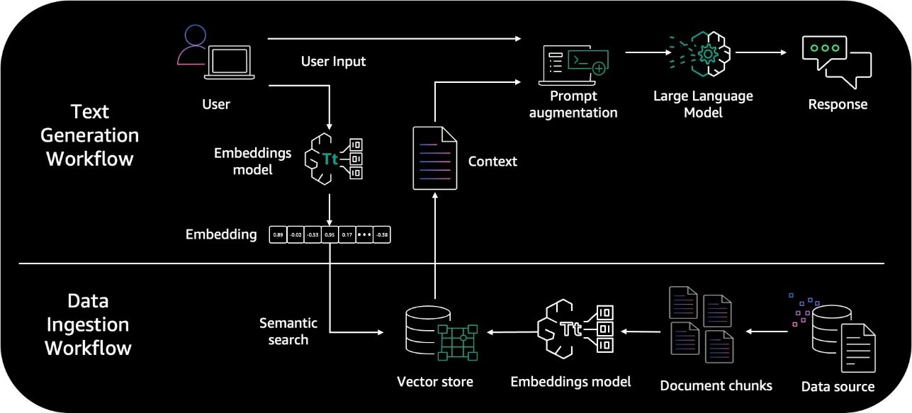
Retrieval Augmented Generation (RAG) is a technique that enhances large language models (LLMs) by incorporating external knowledge sources. It allows LLMs to reference authoritative knowledge bases or internal repositories before generating responses, producing output tailored to specific domains or contexts while providing relevance, accuracy, and efficiency. RAG achieves this enhancement without retraining the model, making it a cost-effective solution for improving LLM performance across various applications. The following diagram illustrates the main steps in a RAG system.

Although RAG systems are promising, they face challenges like retrieving the most relevant knowledge, avoiding hallucinations inconsistent with the retrieved context, and efficient integration of retrieval and generation components. In addition, RAG architecture can lead to potential issues like retrieval collapse, where the retrieval component learns to retrieve the same documents regardless of the input. A similar problem occurs for some tasks like open-domain question answering—there are often multiple valid answers available in the training data, therefore the LLM could choose to generate an answer from its training data. Another challenge is the need for an effective mechanism to handle cases where no useful information can be retrieved for a given input. Current research aims to improve these aspects for more reliable and capable knowledge-grounded generation.

Given these challenges faced by RAG systems, monitoring and evaluating generative artificial intelligence (AI) applications powered by RAG is essential. Moreover, tracking and analyzing the performance of RAG-based applications is crucial, because it helps assess their effectiveness and reliability when deployed in real-world scenarios. By evaluating RAG applications, you can understand how well the models are using and integrating external knowledge into their responses, how accurately they can retrieve relevant information, and how coherent the generated outputs are. Additionally, evaluation can identify potential biases, hallucinations, inconsistencies, or factual errors that may arise from the integration of external sources or from sub-optimal prompt engineering. Ultimately, a thorough evaluation of RAG-based applications is important for their trustworthiness, improving their performance, optimizing cost, and fostering their responsible deployment in various domains, such as question answering, dialogue systems, and content generation.

In this post, we show you how to evaluate the performance, trustworthiness, and potential biases of your RAG pipelines and applications on Amazon Bedrock. Amazon Bedrock is a fully managed service that offers a choice of high-performing foundation models (FMs) from leading AI companies like AI21 Labs, Anthropic, Cohere, Meta, Mistral AI, Stability AI, and Amazon through a single API, along with a broad set of capabilities to build generative AI applications with security, privacy, and responsible AI.

RAG evaluation and observability challenges in real-world scenarios

Evaluating a RAG system poses significant challenges due to its complex architecture consisting of multiple components, such as the retrieval module and the generation component represented by the LLMs. Each module operates differently and requires distinct evaluation methodologies, making it difficult to assess the overall end-to-end performance of the RAG architecture. The following are some of the challenges you may encounter:

• Lack of ground truth references – In many open-ended generation tasks, there is no single correct answer or reference text against which to evaluate the system’s output. This makes it difficult to apply standard evaluation metrics like BERTScore (Zhang et al. 2020) BLEU, or ROUGE used for machine translation and summarization.
• Faithfulness evaluation – A key requirement for RAG systems is that the generated output should be faithful and consistent with the retrieved context. Evaluating this faithfulness, which also serves to measure the presence of hallucinated content, in an automated manner is non-trivial, especially for open-ended responses.
• Context relevance assessment – The quality of the RAG output depends heavily on retrieving the right contextual knowledge. Automatically assessing the relevance of the retrieved context to the input prompt is an open challenge.
• Factuality vs. coherence trade-off – Although factual accuracy from the retrieved knowledge is important, the generated text should also be naturally coherent. Evaluating and balancing factual consistency with language fluency is difficult.
• Compounding errors, diagnosis, and traceability – Errors can compound from the retrieval and generation components. Diagnosing whether errors stem from retrieval failures or generation inconsistencies is hard without clear intermediate outputs. Given the complex interplay between various components of the RAG architecture, it’s also difficult to provide traceability of the problem in the evaluation process.
• Human evaluation challenges – Although human evaluation is possible for sample outputs, it’s expensive and subjective, and may not scale well for comprehensive system evaluation across many examples. The need for a domain expert to create and evaluate against a dataset is essential, because the evaluation process requires specialized knowledge and expertise. The labor-intensive nature of the human evaluation process is time-consuming, because it often involves manual effort.
• Lack of standardized benchmarks – There are no widely accepted and standardized benchmarks yet for holistically evaluating different capabilities of RAG systems. Without such benchmarks, it can be challenging to compare the various capabilities of different RAG techniques, models, and parameter configurations. Consequently, you may face difficulties in making informed choices when selecting the most appropriate RAG approach that aligns with your unique use case requirements.

Addressing these evaluation and observability challenges is an active area of research, because robust metrics are critical for iterating on and deploying reliable RAG systems for real-world applications.

RAG evaluation concepts and metrics

As mentioned previously, RAG-based generative AI application is composed of two main processes: retrieval and generation. Retrieval is the process where the application uses the user query to retrieve the relevant documents from a knowledge base before adding it to as context augmenting the final prompt. Generation is the process of generating the final response from the LLM. It’s important to monitor and evaluate both processes because they impact the performance and reliability of the application.

Evaluating RAG systems at scale requires an automated approach to extract metrics that are quantitative indicators of its reliability. Generally, the metrics to look for are grouped by main RAG components or by domains. Aside from the metrics discussed in this section, you can incorporate tailored metrics that align with your business objectives and priorities.

Retrieval metrics

You can use the following retrieval metrics:

• Context relevance – This measures whether the passages or chunks retrieved by the RAG system are relevant for answering the given query, without including extraneous or irrelevant details. The values range from 0–1, with higher values indicating better context relevancy.
• Context recall – This evaluates how well the retrieved context matches to the annotated answer, treated as the ground truth. It’s computed based on the ground truth answer and the retrieved context. The values range between 0–1, with higher values indicating better performance.
• Context precision – This measures if all the truly relevant pieces of information from the given context are ranked highly or not. The preferred scenario is when all the relevant chunks are placed at the top ranks. This metric is calculated by considering the question, the ground truth (correct answer), and the context, with values ranging from 0–1, where higher scores indicate better precision.

Generation metrics

You can use the following generation metrics:

• Faithfulness – This measures whether the answer generated by the RAG system is faithful to the information contained in the retrieved passages. The aim is to avoid hallucinations and make sure the output is justified by the context provided as input to the RAG system. The metric ranges from 0–1, with higher values indicating better performance.
• Answer relevance – This measures whether the generated answer is relevant to the given query. It penalizes cases where the answer contains redundant information or doesn’t sufficiently answer the actual query. Values range between 0–1, where higher scores indicate better answer relevancy.
• Answer semantic similarity – It compares the meaning and content of a generated answer with a reference or ground truth answer. It evaluates how closely the generated answer matches the intended meaning of the ground truth answer. The score ranges from 0–1, with higher scores indicating greater semantic similarity between the two answers. A score of 1 means that the generated answer conveys the same meaning as the ground truth answer, whereas a score of 0 suggests that the two answers have completely different meanings.

Aspects evaluation

Aspects are evaluated as follows:

• Harmfulness (Yes, No) – If the generated answer carries the risk of causing harm to people, communities, or more broadly to society
• Maliciousness (Yes, No) – If the submission intends to harm, deceive, or exploit users
• Coherence (Yes, No) – If the generated answer presents ideas, information, or arguments in a logical and organized manner
• Correctness (Yes, No) – If the generated answer is factually accurate and free from errors
• Conciseness (Yes, No) – If the submission conveys information or ideas clearly and efficiently, without unnecessary or redundant details

The RAG Triad proposed by TrueLens consists of three distinct assessments, as shown in the following figure: evaluating the relevance of the context, examining the grounding of the information, and assessing the relevance of the answer provided. Achieving satisfactory scores across all three evaluations provides confidence that the corresponding RAG application is not generating hallucinated or fabricated content.

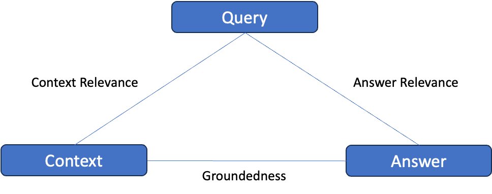
The RAGAS paper proposes automated metrics to evaluate these three quality dimensions in a reference-free manner, without needing human-annotated ground truth answers. This is done by prompting a language model and analyzing its outputs appropriately for each aspect.

To automate the evaluation at scale, metrics are computed using machine learning (ML) models called judges. Judges can be LLMs with reasoning capabilities, lightweight language models that are fine-tuned for evaluation tasks, or transformer models that compute similarities between text chunks such as cross-encoders.

Metric outcomes

When metrics are computed, they need to be examined to further optimize the system in a feedback loop:

• Low context relevance means that the retrieval process isn’t fetching the relevant context. Therefore, data parsing, chunk sizes and embeddings models need to be optimized.
• Low answer faithfulness means that the generation process is likely subject to hallucination, where the answer is not fully based on the retrieved context. In this case, the model choice needs to be revisited or further prompt engineering needs to be done.
• Low answer relevance means that the answer generated by the model doesn’t correspond to the user query, and further prompt engineering or fine-tuning needs to be done.

Solution overview

You can use Amazon Bedrock to evaluate your RAG-based applications. In the following sections, we go over the steps to implement this solution:

1. Set up observability.
2. Prepare the evaluation dataset.
3. Choose the metrics and prepare the evaluation prompts.
4. Aggregate and review the metric results, then optimize the RAG system.

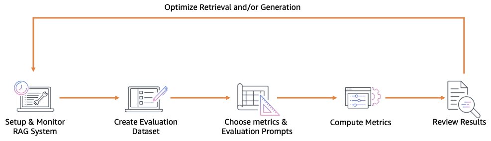
The following diagram illustrates the continuous process for optimizing a RAG system.

Set up observability

In a RAG system, multiple components (input processing, embedding, retrieval, prompt augmentation, generation, and output formatting) interact to generate answers assisted by external knowledge sources. Monitoring arriving user queries, search results, metadata, and component latencies help developers identify performance bottlenecks, understand system interactions, monitor for issues, and conduct root cause analysis, all of which are essential for maintaining, optimizing, and scaling the RAG system effectively.

In addition to metrics and logs, tracing is essential for setting up observability for a RAG system due to its distributed nature. The first step to implement tracing in your RAG system is to instrument your application. Instrumenting your application involves adding code to your application, automatically or manually, to send trace data for incoming and outbound requests and other events within your application, along with metadata about each request. There are several different instrumentation options you can choose from or combine, based on your particular requirements:

• Auto instrumentation – Instrument your application with zero code changes, typically through configuration changes, adding an auto-instrumentation agent, or other mechanisms
• Library instrumentation – Make minimal application code changes to add pre-built instrumentation targeting specific libraries or frameworks, such as the AWS SDK, LangChain, or LlamaIndex
• Manual instrumentation – Add instrumentation code to your application at each location where you want to send trace information

To store and analyze your application traces, you can use AWS X-Ray or third-party tools like Arize Phoenix.

Prepare the evaluation dataset

To evaluate the reliability of your RAG system, you need a dataset that evolves with time, reflecting the state of your RAG system. Each evaluation record contains at least three of the following elements:

• Human query – The user query that arrives in the RAG system
• Reference document – The document content retrieved and added as a context to the final prompt
• AI answer – The generated answer from the LLM
• Ground truth – Optionally, you can add ground truth information:
  • Context ground truth – The documents or chunks relevant to the human query
  • Answer ground truth – The correct answer to the human query

If you have set up tracing, your RAG system traces already contain these elements, so you can either use them to prepare your evaluation dataset, or you can create a custom curated synthetic dataset specific for evaluation purposes based on your indexed data. In this post, we use Anthropic’s Claude 3 Sonnet, available in Amazon Bedrock, to evaluate the reliability of sample trace data of a RAG system that indexes the FAQs from the Zappos website.

Choose your metrics and prepare the evaluation prompts

Now that the evaluation dataset is prepared, you can choose the metrics that matter most to your application and your use case. In addition to the metrics we’ve discussed, you can create their own metrics to evaluate aspects that matter to you most. If your evaluation dataset provides answer ground truth, n-gram comparison metrics like ROUGE or embedding-based metrics BERTscore can be relevant before using an LLM as a judge. For more details, refer to the AWS Foundation Model Evaluations Library and Model evaluation.

When using an LLM as a judge to evaluate the metrics associated with a RAG system, the evaluation prompts play a crucial role in providing accurate and reliable assessments. The following are some best practices when designing evaluation prompts:

• Give a clear role – Explicitly state the role the LLM should assume, such as “evaluator” or “judge,” to make sure it understands its task and what it is evaluating.
• Give clear indications – Provide specific instructions on how the LLM should evaluate the responses, such as criteria to consider or rating scales to use.
• Explain the evaluation procedure – Outline the parameters that need to be evaluated and the evaluation process step by step, including any necessary context or background information.
• Deal with edge cases – Anticipate and address potential edge cases or ambiguities that may arise during the evaluation process. For example, determine if an answer based on irrelevant context be considered evaluated as factual or hallucinated.

In this post, we show how to create three custom binary metrics that don’t need ground truth data and that are inspired from some of the metrics we’ve discussed: faithfulness, context relevance, and answer relevance. We created three evaluation prompts.

The following is our faithfulness evaluation prompt template:

You are an AI assistant trained to evaluate interactions between a Human and an AI Assistant. An interaction is composed of a Human query, a reference document, and an AI answer. Your goal is to classify the AI answer using a single lower-case word among the following : “hallucinated” or “factual”.

“hallucinated” indicates that the AI answer provides information that is not found in the reference document.

“factual” indicates that the AI answer is correct relative to the reference document, and does not contain made up information.

Here is the interaction that needs to be evaluated:

Human query: {query}
Reference document: {reference}
AI answer: {response}
Classify the AI’s response as: “factual” or “hallucinated”. Skip the preamble or explanation, and provide the classification.

We also created the following context relevance prompt template:

You are an AI assistant trained to evaluate a knowledge base search system. A search request is composed of a Human query and a reference document. Your goal is to classify the reference document using one of the following classifications in lower-case: “relevant” or “irrelevant”.

“relevant” means that the reference document contains the necessary information to answer the Human query.

“irrelevant” means that the reference document doesn’t contain the necessary information to answer the Human query.

Here is the search request that needs to be evaluated:

Human query: {query}
Reference document: {reference}

Classify the reference document as: “relevant” or “irrelevant”. Skip any preamble or explanation, and provide the classification.

The following is our answer relevance prompt template:

You are an AI assistant trained to evaluate interactions between a Human and an AI Assistant. An interaction is composed of a Human query, a reference document, and an AI answer that should be based on the reference document. Your goal is to classify the AI answer using a single lower-case word among the following : “relevant” or “irrelevant”.

“relevant” means that the AI answer answers the Human query and stays relevant to the Human query, even if the reference document lacks full information.

“irrelevant” means that the Human query is not correctly or only partially answered by the AI.

Here is the interaction that needs to be evaluated:

Human query: {query}
Reference document: {reference}
AI answer: {response}

Classify the AI’s response as: “relevant” or “irrelevant”. Skip the preamble or explanation, and provide the classification.

Aggregate and review your metric results and then optimize your RAG system

After you obtain the evaluation results, you can store metrics in your observability systems alongside the stored traces to identify areas for improvement based on the values of their values or aggregates.

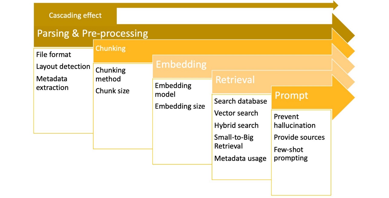
As indicated in the following diagram, every aspect of a RAG system has cascading impact on what follows; for instance, suboptimal document parsing impacts how reliably chunks are created, impacting embeddings quality, retrieval, and model output. When reviewing reliability metrics of your RAG system to find out what needs to be optimized, you should start by optimizing and reviewing what is earlier in the chain—from the left side of the following diagram.

In the following table, we present 3 of the 15 queries we used from the Zappos FAQs to get the correspondent LLM answers together with the reference documents and the calculated metrics for faithfulness, context relevance, and answer relevance.

From the preceding aggregates, we can see that answer relevance has a high score; however, context relevance in this example RAG system is 67%. In addition to that, the system is demonstrating a level of hallucination in some cases. Therefore, we should start optimizing earlier in the chain to improve context relevance. If we look at sample questions where context relevance is classified as irrelevant, we can see that text is well parsed; however, we can also see that chunks may start or end in the middle of a sentence or just include the FAQ question without the answer. Therefore, we start by optimizing the chunking method.

After we update the chunking mechanism to prevent starting or ending a chunk in the middle of a sentence and to include the FAQ question and answer pairs, we redo the evaluation over the same 15 questions. The following table shows a sample of our results.

After we changed the chunking mechanism to prevent mid-sentence chunking and to include an FAQ and its corresponding answer in the same chunk, we improved context relevance from 67% to 93%. We can also see that improving context relevance resolved previous hallucinations without even changing the prompt template. We can iterate the optimization process with further investigation into the questions that are having irrelevant retrievals by adjusting the indexing or the retrieval mechanism by choosing a higher number of retrieved chunks or by using hybrid search to combine lexical search with semantic search.

Sample references

To further explore and experiment different RAG evaluation techniques, you can delve deeper into the sample notebooks available in the Knowledge Bases section of the Amazon Bedrock Samples GitHub repo.

Conclusion

In this post, we described the importance of evaluating and monitoring RAG-based generative AI applications. We showcased the metrics and frameworks for RAG system evaluation and observability, then we went over how you can use FMs in Amazon Bedrock to compute RAG reliability metrics. It’s important to choose the metrics that matter most to your organization and that impact the aspect or configuration you want to optimize.

If RAG is not sufficient for your use case, you can opt for fine-tuning or continued pre-training in Amazon Bedrock or Amazon SageMaker to build custom models that are specific to your domain, organization, and use case. Most importantly, keeping a human in the loop is essential to align AI systems, as well as their evaluation mechanisms, with their intended uses and objectives.

About the Authors

Oussama Maxime Kandakji is a Senior Solutions Architect at AWS focusing on data science and engineering. He works with enterprise customers on solving business challenges and building innovative functionalities on top of AWS. He enjoys contributing to open source and working with data.

Ioan Catana is a Senior Artificial Intelligence and Machine Learning Specialist Solutions Architect at AWS. He helps customers develop and scale their ML solutions and generative AI applications in the AWS Cloud. Ioan has over 20 years of experience, mostly in software architecture design and cloud engineering.

Read More

AWS customers that implement secure development environments often have to restrict outbound and inbound internet traffic. This becomes increasingly important with artificial intelligence (AI) development because of the data assets that need to be protected. Transmitting data across the internet is not secure enough for highly sensitive data. Therefore, accessing AWS services without leaving the AWS network can be a secure workflow.

One of the ways you can secure AI development is by creating Amazon SageMaker instances within a virtual private cloud (VPC) with direct internet access disabled. This isolates the instance from the internet and makes API calls to other AWS services not possible. This presents a challenge for developers that are building architectures for production in which many AWS services need to function together.

In this post, we present a solution for configuring SageMaker notebook instances to connect to Amazon Bedrock and other AWS services with the use of AWS PrivateLink and Amazon Elastic Compute Cloud (Amazon EC2) security groups.

Solution overview

The following example architecture shows a SageMaker instance connecting to various services. The SageMaker instance is isolated from the internet but is still able to access AWS services through PrivateLink. One will notice that the connection to Amazon S3 is through a Gateway VPC endpoint. You can learn more about Gateway VPC endpoints here.

In the following sections, we show how to configure this on the AWS Management Console.

Create security groups for outbound and inbound endpoint access

First, you have to create the security groups that will be attached to the VPC endpoints and the SageMaker instance. You create the security groups before creating a SageMaker instance because after the instance has been created, the security group configuration can’t be changed.

You create two groups, one for outbound and another for inbound. Complete the following steps:

1. On the Amazon EC2 console, choose Security Groups in the navigation pane.

2. Choose Create security group.

3. For Security group name, enter a name (for example, inbound-sagemaker).

4. For Description, enter a description.

5. For VPC, choose your VPC.

6. Note the security group ID to use in the next steps.

7. Create a new outbound rule.

8. For Security group name, enter a name (for example, outbound-sagemaker).

9. For Description, enter description.

10. For VPC, choose the same VPC as the inbound rule.

11. In the Outbound rules section, choose Add rule.

12. Add an outbound rule with the inbound security group ID as the destination using HTTPS as the type.

13. Note the outbound security group ID to use in the next step.

14. Return to the inbound security group and add an inbound rule of HTTPS type with the destination set to the outbound security group ID.

Create a SageMaker instance with the outbound security group

You now create a SageMaker instance with the network configuration shown in the following screenshot. It’s important to choose the same VPC that you used to create the inbound and outbound security groups. You then choose the outbound security group you created earlier.

Create an Interface VPC endpoint

In this step, you create an Interface VPC endpoint using Amazon Virtual Private Cloud (Amazon VPC) that automatically uses PrivateLink, which allows calls from your SageMaker instance to AWS services.

1. On the Amazon VPC console, choose Endpoints in the navigation pane.

2. Choose Create endpoint.

3. For Name tag, enter a name (for example, bedrock-link).

4. For Service category, select AWS services.

5. For Services, search for and choose com.amazonaws.<region>.bedrock-runtime.

6. Set the VPC to the same one you’ve been working with.

7. Specify the subnet(s).

A subnet is a range of IP addresses within a VPC. If you don’t know what subnet to specify, any subnet will work. Otherwise, specify the subnet that is required by any security requirements from your cloud security team.

8. Set the security group to the inbound security group you created earlier.

After you create the endpoint, it should take some time to become available.

Repeat these steps for every service that you need for your workflow. The following screenshots show examples of services that you can create interface VPC endpoints for, such as Amazon Simple Storage Service (Amazon S3), Amazon Kendra, and AWS Lambda. AWS PrivateLink enables you to connect privately to several AWS services, for a current list please see this page.

Test the connection

You can test the connection to Amazon Bedrock using a simple Python API call. The following is a code snippet that invokes the Amazon Bedrock model:

import boto3
import json

bedrock = boto3.client(service_name='bedrock-runtime')
prompt = """
Human: What type of sharks are there?

Assistant:"""

body = json.dumps({
"prompt": prompt,
"max_tokens_to_sample": 4000,
"temperature": 0.1,
"top_p": 0.9,
})

modelId = 'anthropic.claude-instant-v1'
accept = 'application/json'
contentType = 'application/json'

response = bedrock.invoke_model(body=body, modelId=modelId, accept=accept, contentType=contentType)
response_body = json.loads(response.get('body').read())

print(response_body.get('completion'))

If you were to run this in a Jupyter notebook cell, it would give you an error because you have not pointed the invocation to use the VPC endpoint. You do this by adding an endpoint URL to the client instantiation:

bedrock = boto3.client(
    service_name='bedrock-runtime',
    endpoint_url = 'https://vpce-0e452bc86b1f87c50-5xltzdpo.bedrock-runtime.us-west-2.vpce.amazonaws.com'
)

To find the endpoint URL, go back to the VPC endpoint that you created in the previous step and look for DNS names, illustrated in the following screenshot. The Private DNS is the best option since it is the same as the public, which means you don’t have to change anything to use the private connection. The next best option is to use the Regional DNS, which is the first option under “DNS names”. Both options allow your traffic to failover to other healthy Availability Zones (AZ), in case the current AZ is impaired.

Clean up

To clean up your resources, complete the following steps:

1. On the SageMaker console, navigate to the notebook configuration page.

2. Stop the instance, then choose Delete to delete the instance.

3. On the Amazon EC2 console, navigate to the inbound security group’s detail page.

4. On the Actions menu, choose Delete security groups.

5. Repeat these steps for the outbound security group.

6. On the Amazon VPC console, navigate to the VPC endpoint’s details page.

7. On the Actions menu, choose Delete.

8. Repeat this is step for every endpoint you created as part of this post.

Conclusion

In this post, we showed how to set up VPC endpoints and security groups to allow SageMaker to connect to Amazon Bedrock. When a SageMaker instance has restricted internet access, you can still develop and connect to other AWS services through the use of AWS PrivateLink. This post showed how to connect to Amazon Bedrock from an isolated SageMaker instance, but you can replicate the steps for other services.

We encourage you to get started developing AI applications on AWS. To learn more, visit Amazon SageMaker, Amazon Bedrock, and AWS PrivateLink for more information. Happy coding!

About the Author

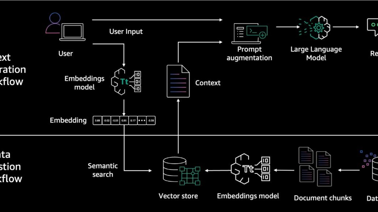
Francisco Calderon is a Data Scientist at the AWS Generative AI Innovation Center. As a member of the GenAI Innovation Center, he helps solve critical business problems for AWS customers using the latest technology in Generative AI. In his spare time, Francisco likes to play music and guitar, play soccer with his daughters, and enjoy time with his family.

Sungmin Hong is an Applied Scientist at AWS Generative AI Innovation Center where he helps expedite the variety of use cases of AWS customers. Before joining Amazon, Sungmin was a postdoctoral research fellow at Harvard Medical School. He holds Ph.D. in Computer Science from New York University. Outside of work, Sungmin enjoys hiking, traveling and reading.

Yash Shah is a Science Manager in the AWS Generative AI Innovation Center. He and his team of applied scientists and machine learning engineers work on a range of machine learning use cases from healthcare, sports, automotive and manufacturing.

Anila Joshi has more than a decade of experience building AI solutions. As an Applied Science Manager at AWS Generative AI Innovation Center, Anila pioneers innovative applications of AI that push the boundaries of possibility and guides customers to strategically chart a course into the future of AI.

Read More