NVIDIA Announces Isaac GR00T Blueprint to Accelerate Humanoid Robotics Development

NVIDIA Announces Isaac GR00T Blueprint to Accelerate Humanoid Robotics Development

Over the next two decades, the market for humanoid robots is expected to reach $38 billion. To address this significant demand, particularly in industrial and manufacturing sectors, NVIDIA is releasing a collection of robot foundation models, data pipelines and simulation frameworks to accelerate next-generation humanoid robot development efforts.

Announced by NVIDIA founder and CEO Jensen Huang today at the CES trade show, the NVIDIA Isaac GR00T Blueprint for synthetic motion generation helps developers generate exponentially large synthetic motion data to train their humanoids using imitation learning.

Imitation learning — a subset of robot learning — enables humanoids to acquire new skills by observing and mimicking expert human demonstrations. Collecting these extensive, high-quality datasets in the real world is tedious, time-consuming and often prohibitively expensive. Implementing the Isaac GR00T blueprint for synthetic motion generation allows developers to easily generate exponentially large synthetic datasets from just a small number of human demonstrations.

Starting with the GR00T-Teleop workflow, users can tap into the Apple Vision Pro to capture human actions in a digital twin. These human actions are mimicked by a robot in  simulation and recorded for use as ground truth.

The GR00T-Mimic workflow then multiplies the captured human demonstration into a larger synthetic motion dataset. Finally, the GR00T-Gen workflow, built on the NVIDIA Omniverse and NVIDIA Cosmos platforms, exponentially expands this dataset through domain randomization and 3D upscaling.

The dataset can then be used as an input to the robot policy, which teaches robots how to move and interact with their environment effectively and safely in NVIDIA Isaac Lab, an open-source and modular framework for robot learning.

World Foundation Models Narrow the Sim-to-Real Gap 

NVIDIA also announced Cosmos at CES, a platform featuring a family of open, pretrained world foundation models purpose-built for generating physics-aware videos and world states for physical AI development. It includes autoregressive and diffusion models in a variety of sizes and input data formats. The models were trained on 18 quadrillion tokens, including 2 million hours of autonomous driving, robotics, drone footage and synthetic data.

In addition to helping generate large datasets, Cosmos can reduce the simulation-to-real gap by upscaling images from 3D to real. Combining Omniverse — a developer platform of application programming interfaces and microservices for building 3D applications and services — with Cosmos is critical, because it helps minimize potential hallucinations commonly associated with world models by providing crucial safeguards through its highly controllable, physically accurate simulations.

An Expanding Ecosystem 

Collectively, NVIDIA Isaac GR00T, Omniverse and Cosmos are helping physical AI and humanoid innovation take a giant leap forward. Major robotics companies have started adopting and demonstrated results with Isaac GR00T, including Boston Dynamics and Figure.

Humanoid software, hardware and robot manufacturers can apply for early access to NVIDIA’s humanoid robot developer program.

Watch the CES opening keynote from NVIDIA founder and CEO Jensen Huang, and stay up to date by subscribing to the newsletter and following NVIDIA Robotics on LinkedIn, Instagram, X and Facebook.

See notice regarding software product information.

Read More

NVIDIA Makes Cosmos World Foundation Models Openly Available to Physical AI Developer Community

NVIDIA Makes Cosmos World Foundation Models Openly Available to Physical AI Developer Community

NVIDIA Cosmos, a platform for accelerating physical AI development, introduces a family of world foundation models — neural networks that can predict and generate physics-aware videos of the future state of a virtual environment — to help developers build next-generation robots and autonomous vehicles (AVs).

World foundation models, or WFMs, are as fundamental as large language models. They use input data, including text, image, video and movement, to generate and simulate virtual worlds in a way that accurately models the spatial relationships of objects in the scene and their physical interactions.

Announced today at CES, NVIDIA is making available the first wave of Cosmos WFMs for physics-based simulation and synthetic data generation — plus state-of-the-art tokenizers, guardrails, an accelerated data processing and curation pipeline, and a framework for model customization and optimization.

Researchers and developers, regardless of their company size, can freely use the Cosmos models under NVIDIA’s permissive open model license that allows commercial usage. Enterprises building AI agents can also use new open NVIDIA Llama Nemotron and Cosmos Nemotron models, unveiled at CES.

The openness of Cosmos’ state-of-the-art models unblocks physical AI developers building robotics and AV technology and enables enterprises of all sizes to more quickly bring their physical AI applications to market. Developers can use Cosmos models directly to generate physics-based synthetic data, or they can harness the NVIDIA NeMo framework to fine-tune the models with their own videos for specific physical AI setups.

Physical AI leaders — including robotics companies 1X, Agility Robotics and XPENG, and AV developers Uber and Waabi  — are already working with Cosmos to accelerate and enhance model development.

Developers can preview the first Cosmos autoregressive and diffusion models on the NVIDIA API catalog, and download the family of models and fine-tuning framework from the NVIDIA NGC catalog and Hugging Face.

World Foundational Models for Physical AI

Cosmos world foundation models are a suite of open diffusion and autoregressive transformer models for physics-aware video generation. The models have been trained on 9,000 trillion tokens from 20 million hours of real-world human interactions, environment, industrial, robotics and driving data.

The models come in three categories: Nano, for models optimized for real-time, low-latency inference and edge deployment; Super, for highly performant baseline models; and Ultra, for maximum quality and fidelity, best used for distilling custom models.

When paired with NVIDIA Omniverse 3D outputs, the diffusion models generate controllable, high-quality synthetic video data to bootstrap training of robotic and AV perception models. The autoregressive models predict what should come next in a sequence of video frames based on input frames and text. This enables real-time next-token prediction, giving physical AI models the foresight to predict their next best action.

Developers can use Cosmos’ open models for text-to-world and video-to-world generation. Versions of the diffusion and autoregressive models, with between 4 and 14 billion parameters each, are available now on the NGC catalog and Hugging Face.

Also available are a 12-billion-parameter upsampling model for refining text prompts, a 7-billion-parameter video decoder optimized for augmented reality, and guardrail models to ensure responsible, safe use.

To demonstrate opportunities for customization, NVIDIA is also releasing fine-tuned model samples for vertical applications, such as generating multisensor views for AVs.

Advancing Robotics, Autonomous Vehicle Applications

Cosmos world foundation models can enable synthetic data generation to augment training datasets, simulation to test and debug physical AI models before they’re deployed in the real world, and reinforcement learning in virtual environments to accelerate AI agent learning.

Developers can generate massive amounts of controllable, physics-based synthetic data by conditioning Cosmos with composed 3D scenes from NVIDIA Omniverse.

Waabi, a company pioneering generative AI for the physical world, starting with autonomous vehicles, is evaluating the use of Cosmos for the search and curation of video data for AV software development and simulation. This will further accelerate the company’s industry-leading approach to safety, which is based on Waabi World, a generative AI simulator that can create any situation a vehicle might encounter with the same level of realism as if it happened in the real world.

In robotics, WFMs can generate synthetic virtual environments or worlds to provide a less expensive, more efficient and controlled space for robot learning. Embodied AI startup Hillbot is boosting its data pipeline by using Cosmos to generate terabytes of high-fidelity 3D environments. This AI-generated data will help the company refine its robotic training and operations, enabling faster, more efficient robotic skilling and improved performance for industrial and domestic tasks.

In both industries, developers can use NVIDIA Omniverse and Cosmos as a multiverse simulation engine, allowing a physical AI policy model to simulate every possible future path it could take to execute a particular task — which in turn helps the model select the best of these paths.

Data curation and the training of Cosmos models relied on thousands of NVIDIA GPUs through NVIDIA DGX Cloud, a high-performance, fully managed AI platform that provides accelerated computing clusters in every leading cloud.

Developers adopting Cosmos can use DGX Cloud for an easy way to deploy Cosmos models, with further support available through the NVIDIA AI Enterprise software platform.

Customize and Deploy With NVIDIA Cosmos

In addition to foundation models, the Cosmos platform includes a data processing and curation pipeline powered by NVIDIA NeMo Curator and optimized for NVIDIA data center GPUs.

Robotics and AV developers collect millions or billions of hours of real-world recorded video, resulting in petabytes of data. Cosmos enables developers to process 20 million hours of data in just 40 days on NVIDIA Hopper GPUs, or as little as 14 days on NVIDIA Blackwell GPUs. Using unoptimized pipelines running on a CPU system with equivalent power consumption, processing the same amount of data would take over three years.

The platform also features a suite of powerful video and image tokenizers that can convert videos into tokens at different video compression ratios for training various transformer models.

The Cosmos tokenizers deliver 8x more total compression than state-of-the-art methods and 12x faster processing speed, which offers superior quality and reduced computational costs in both training and inference. Developers can access these tokenizers, available under NVIDIA’s open model license, via Hugging Face and GitHub.

Developers using Cosmos can also harness model training and fine-tuning capabilities offered by NeMo framework, a GPU-accelerated framework that enables high-throughput AI training.

Developing Safe, Responsible AI Models

Now available to developers under the NVIDIA Open Model License Agreement, Cosmos was developed in line with NVIDIA’s trustworthy AI principles, which include nondiscrimination, privacy, safety, security and transparency.

The Cosmos platform includes Cosmos Guardrails, a dedicated suite of models that, among other capabilities, mitigates harmful text and image inputs during preprocessing and screens generated videos during postprocessing for safety. Developers can further enhance these guardrails for their custom applications.

Cosmos models on the NVIDIA API catalog also feature an inbuilt watermarking system that enables identification of AI-generated sequences.

NVIDIA Cosmos was developed by NVIDIA Research. Read the research paper, “Cosmos World Foundation Model Platform for Physical AI,” for more details on model development and benchmarks. Model cards providing additional information are available on Hugging Face.

Learn more about world foundation models in an AI Podcast episode, airing Jan. 7, that features Ming-Yu Liu, vice president of research at NVIDIA. 

Get started with NVIDIA Cosmos and join NVIDIA at CES. Watch the Cosmos demo and Huang’s keynote below: 

See notice regarding software product information.

Read More

PC Gaming in the Cloud Goes Everywhere With New Devices and AAA Games on GeForce NOW

PC Gaming in the Cloud Goes Everywhere With New Devices and AAA Games on GeForce NOW

GeForce NOW turns any device into a GeForce RTX gaming PC, and is bringing cloud gaming and AAA titles to more devices and regions.

Announced today at the CES trade show, gamers will soon be able to play titles from their Steam library at GeForce RTX quality with the launch of a native GeForce NOW app for the Steam Deck. NVIDIA is working to bring cloud gaming to the popular PC gaming handheld device later this year.

In collaboration with Apple, Meta and ByteDance, NVIDIA is expanding GeForce NOW cloud gaming to Apple Vision Pro spatial computers, Meta Quest 3 and 3S and Pico virtual- and mixed-reality devices — with all the bells and whistles of NVIDIA technologies, including ray tracing and NVIDIA DLSS.

In addition, NVIDIA is launching the first GeForce RTX-powered data center in India, making gaming more accessible around the world.

Plus, GeForce NOW’s extensive library of over 2,100 supported titles is expanding with highly anticipated AAA titles. DOOM: The Dark Ages and Avowed will join the cloud when they launch on PC this year.

RTX on Deck

The Steam Deck’s portability paired with GeForce NOW opens up new possibilities for high-fidelity gaming everywhere. The native GeForce NOW app will offer up to 4K resolution and 60 frames per second with high dynamic range on Valve’s innovative Steam Deck handheld when connected to a TV, streaming from GeForce RTX-powered gaming rigs in the cloud.

Last year, GeForce NOW rolled out a beta installation method that was eagerly welcomed by the gaming community. Later this year, members will be able to download the native GeForce NOW app and install it on Steam Deck.

Steam Deck gamers can gain access to all the same benefits as GeForce RTX 4080 GPU owners with a GeForce NOW Ultimate membership, including NVIDIA DLSS 3 technology for the highest frame rates and NVIDIA Reflex for ultra-low latency. Because GeForce NOW streams from an RTX gaming rig in the cloud, the Steam Deck uses less processing power, which extends battery life compared with playing locally.

The streaming experience with GeForce NOW looks stunning, whichever way Steam Deck users want to play — whether that’s in handheld mode for HDR-quality graphics, connected to a monitor for up to 1440p 120 fps HDR or hooked up to a TV for big-screen streaming at up to 4K 60 HDR. GeForce NOW members can take advantage of RTX ON with the Steam Deck for photorealistic gameplay on supported titles, as well as HDR10 and SDR10 when connected to a compatible display for richer, more accurate color gradients.

Get ready for major upgrades to streaming on the go when the GeForce NOW app launches on the Steam Deck later this year.

Stream Beyond Reality

Get immersed in a new dimension of big-screen gaming as GeForce NOW brings AAA titles to life on Apple Vision Pro spatial computers, Meta Quest 3 and 3S and Pico virtual- and mixed-reality headsets. Later this month, these supported devices will give members access to an extensive library of games to stream through GeForce NOW by opening the browser to play.geforcenow.com when the newest app update, version 2.0.70, starts rolling out later this month.

Meta Quest 3 to be on GeForce NOW
Jump into a whole new gaming dimension with GeForce NOW.

Members can transform the space around them into a personal gaming theater with GeForce NOW. The streaming experience on these devices will support gamepad-compatible titles for members to play their favorite PC games on a massive virtual screen.

For an even more enhanced visual experience, GeForce NOW Ultimate and Performance members using these devices can tap into RTX and DLSS technologies in supported games. Members will be able to step into a world where games come to life on a grand scale, powered by GeForce NOW technologies.

Land of a Thousand Lights … and Games

India data center to be on GeForce NOW
New year, new data center.

NVIDIA is broadening cloud gaming in India and Latin America. The first GeForce RTX 4080-powered data center will launch in India in the first half of this year. This follows the launch of GeForce NOW in Japan last year, as well as in Colombia and Chile, to be operated by GeForce NOW Alliance partner Digevo.

GeForce RTX-powered gaming in the rapidly growing Indian gaming market will provide the ability to stream AAA games without the latest hardware. Gamers in the region can look forward to the launch of Ultimate memberships, along with all the new games and technological advancements announced at CES.

Send in the Games

AAA content from celebrated publishers is coming to the cloud. Avowed from Obsidian Entertainment, known for iconic titles such as Fallout: New Vegas, will join GeForce NOW. The cloud gaming platform will also bring DOOM: The Dark Ages from id Software, the legendary studio behind the DOOM franchise. All will be available at launch on PC this year.

Avowed to be on GeForce NOW
Get ready to jump into the Living Lands.

Avowed, a first-person fantasy role-playing game, will join the cloud when it launches on PC on Tuesday, Feb. 18. Welcome to the Living Lands, an island full of mysteries and secrets, danger and adventure, choices and consequences and untamed wilderness. Take on the role of an Aedyr Empire envoy tasked with investigating a mysterious plague. Freely combine weapons and magic — harness dual-wield wands, pair a sword with a pistol or opt for a more traditional sword-and-shield approach. In-game companions — which join the players’ parties — have unique abilities and storylines that can be influenced by gamers’ choices.

DOOM: The Dark Ages to be on GeForce NOW
Have a hell of a time in the cloud.

DOOM: The Dark Ages is the single-player, action first-person shooter prequel to the critically acclaimed DOOM (2016) and DOOM Eternal. Play as the DOOM Slayer, the legendary demon-killing warrior fighting endlessly against Hell. Experience the epic cinematic origin story of the DOOM Slayer’s rage this year.

Get ready to play these titles and more at high performance when they join GeForce NOW at launch. Ultimate members will be able to stream at up to 4K resolution and 120 fps with support for NVIDIA DLSS and Reflex technology, and experience the action even on low-powered devices. Keep an eye out on GFN Thursdays for the latest on their release dates in the cloud.

GeForce NOW is making popular devices cloud-gaming-ready while consistently delivering quality titles from top publishers to bring another ultimate year of gaming to members across the globe.

See notice regarding software product information.

Read More

NVIDIA Launches DRIVE AI Systems Inspection Lab, Achieves New Industry Safety Milestones

NVIDIA Launches DRIVE AI Systems Inspection Lab, Achieves New Industry Safety Milestones

A new NVIDIA DRIVE AI Systems Inspection Lab will help automotive ecosystem partners navigate evolving industry standards for autonomous vehicle safety.

The lab, launched today, will focus on inspecting and verifying that automotive partner software and systems on the NVIDIA DRIVE AGX platform meet the automotive industry’s stringent safety and cybersecurity standards, including AI functional safety.

The lab has been accredited by the ANSI National Accreditation Board (ANAB) according to the ISO/IEC 17020 assessment for standards, including:

  • Functional safety (ISO 26262)
  • SOTIF (ISO 21448)
  • Cybersecurity (ISO 21434)
  • UN-R regulations, including UN-R 79, UN-R 13-H, UN-R 152, UN-R 155, UN-R 157 and UN-R 171
  • AI functional safety (ISO PAS 8800 and ISO/IEC TR 5469)

“The launch of this new lab will help partners in the global automotive ecosystem create safe, reliable autonomous driving technology,” said Ali Kani, vice president of automotive at NVIDIA. “With accreditation by ANAB, the lab will carry out an inspection plan that combines functional safety, cybersecurity and AI — bolstering adherence to the industry’s safety standards.”

“ANAB is proud to be the accreditation body for the NVIDIA DRIVE AI Systems Inspection Lab,” said R. Douglas Leonard Jr., executive director of ANAB. “NVIDIA’s comprehensive evaluation verifies the demonstration of competence and compliance with internationally recognized standards, helping ensure that DRIVE ecosystem partners meet the highest benchmarks for functional safety, cybersecurity and AI integration.”

The new lab builds on NVIDIA’s ongoing safety compliance work with Mercedes-Benz and JLR. Inaugural participants in the lab include Continental and Sony SSS-America.

“We are pleased to participate in the newly launched NVIDIA Drive AI Systems Inspection Lab and to further intensify the fruitful, ongoing collaboration between our two companies,” said Nobert Hammerschmidt, head of components business at Continental.

“Self-driving vehicles have the capability to significantly enhance safety on roads,” said Marius Evensen, head of automotive image sensors at Sony SSS-America. “We look forward to working with NVIDIA’s DRIVE AI Systems Inspection Lab to help us deliver the highest levels of safety to our customers.”

“Compliance with functional safety, SOTIF and cybersecurity is particularly challenging for complex systems such as AI-based autonomous vehicles,” said Riccardo Mariani, head of industry safety at NVIDIA. “Through the DRIVE AI Systems Inspection Lab, the correctness of the integration of our partners’ products with DRIVE safety and cybersecurity requirements can be inspected and verified.”

Now open to all NVIDIA DRIVE AGX platform partners, the lab is expected to expand to include additional automotive and robotics products and add a testing component.

Complementing International Automotive Safety Standards

The NVIDIA DRIVE AI Systems Inspection Lab complements the missions of independent third-party certification bodies, including technical service organizations such as TÜV SÜD, TÜV Rheinland and exida, as well as vehicle certification agencies such as VCA and KBA.

Today’s announcement dovetails with recent significant safety certifications and assessments of NVIDIA automotive products:

TÜV SÜD granted the ISO 21434 Cybersecurity Process certification to NVIDIA for its automotive system-on-a-chip, platform and software engineering processes. Upon certification release, the NVIDIA DriveOS 6.0 operating system conforms with ISO 26262 Automotive Safety Integrity Level (ASIL) D standards.

“Meeting cybersecurity process requirements is of fundamental importance in the autonomous vehicle era,” said Martin Webhofer, CEO of TÜV SÜD Rail GmbH. “NVIDIA has successfully established processes, activities and procedures that fulfill the stringent requirements of ISO 21434. Additionally, NVIDIA DriveOS 6.0 conforms to ISO 26262 ASIL D standards, pending final certification activities.”

TÜV Rheinland performed an independent United Nations Economic Commission for Europe safety assessment of NVIDIA DRIVE AV related to safety requirements for complex electronic systems.

“NVIDIA has demonstrated thorough, high-quality, safety-oriented processes and technologies in the context of the assessment of the generic, non-OEM-specific parts of the SAE level 2 NVIDIA DRIVE system,” said Dominik Strixner, global lead functional safety automotive mobility at TÜV Rheinland.

To learn more about NVIDIA’s work in advancing autonomous driving safety, read the NVIDIA Self-Driving Safety Report.

Read More

NVIDIA DRIVE Partners Showcase Latest Mobility Innovations at CES

NVIDIA DRIVE Partners Showcase Latest Mobility Innovations at CES

Leading global transportation companies — spanning the makers of passenger vehicles, trucks, robotaxis and autonomous delivery systems — are turning to the NVIDIA DRIVE AGX platform and AI to build the future of mobility.

NVIDIA’s automotive business provides a range of next-generation highly automated and autonomous vehicle (AV) development technologies, including cloud-based AI training, simulation and in-vehicle compute.

At the CES trade show in Las Vegas this week, NVIDIA’s customers and partners are showcasing their latest mobility innovations built on NVIDIA accelerated computing and AI.

Readying Future Vehicle Roadmaps With NVIDIA DRIVE Thor, Built on NVIDIA Blackwell

The NVIDIA DRIVE AGX Thor system-on-a-chip (SoC), built on the NVIDIA Blackwell architecture, is engineered to handle the transportation industry’s most demanding data-intensive workloads, including those involving generative AI, vision language models and large language models.

DRIVE Ecosystem Partners Transform the Show Floor and Industry at Large

NVIDIA partners are pushing boundaries of automotive innovation with their latest developments and demos, using NVIDIA technologies and accelerated computing to advance everything from sensors, simulation and training to generative AI and teledriving, and include:

Delivering 1,000 teraflops of accelerated compute performance, DRIVE Thor is equipped to accelerate inference tasks that are critical for autonomous vehicles to understand and navigate the world around them, such as recognizing pedestrians, adjusting to inclement weather and more.

At CES, Aurora, Continental and NVIDIA announced a long-term strategic partnership to deploy driverless trucks at scale, powered by the next-generation NVIDIA DRIVE Thor SoC. NVIDIA DRIVE Thor and DriveOS will be integrated into the Aurora Driver, an SAE level 4 autonomous driving system that Continental plans to mass-manufacture in 2027.

Arm, one of NVIDIA’s key technology partners, is the compute platform of choice for a number of innovations at CES. The Arm Neoverse V3AE CPU, designed to meet the specific safety and performance demands of automotive, is integrated with DRIVE Thor. This marks the first implementation of Arm’s next-generation automotive CPU, which combines Arm v9-based technologies with data-center-class single-thread performance, alongside essential safety and security features.

Tried and True — DRIVE Orin Mainstream Adoption Continues

NVIDIA DRIVE AGX Orin, the predecessor of DRIVE Thor, continues to be a production-proven advanced driver-assistance system computer widely used in cars today — delivering 254 trillion operations per second of accelerated compute to process sensor data for safe, real-time driving decisions.

Toyota, the world’s largest automaker, will build its next-generation vehicles on the high-performance, automotive-grade NVIDIA DRIVE Orin SoC, running the safety-certified NVIDIA DriveOS. These vehicles will offer functionally safe advanced driving-assistance capabilities.

At the NVIDIA showcase on the fourth floor of the Fontainebleau, Volvo Cars’ software-defined EX90 and Nuro’s autonomous driving technology — the Nuro Driver platform — will be on display, built on NVIDIA DRIVE AGX.

Other vehicles powered by NVIDIA DRIVE Orin on display during CES include:

  • Zeekr Mix and Zeekr 001, which feature DRIVE Orin will be on display along with the debut of Zeekr’s self-developed ultra-high-performance intelligent driving domain controller that will be built on DRIVE Thor and the NVIDIA Blackwell architecture (LVCC West Hall, booth 5640)
  • Lotus Eletre Carbon (LVCC West Hall, booth 4266 with P3 and 3SS and booth 3500 with HERE)
  • Rivian R1S and Polestar 3 activated with Dolby — vehicles on display and demos available by appointment (Park MGM/NoMad Hotel next to Dolby Live)
  • Lucid Air (LVCC West Hall booth 4964 with SoundHound AI)
Zeekr MIX
Rivian R1S

NVIDIA’s partners will also showcase their automotive solutions built on NVIDIA technologies, including:

  • Arbe: Delivering next-generation, ultra-high-definition radar technology, integrating with NVIDIA DRIVE AGX to revolutionize radar-based free-space mapping with cutting-edge AI capabilities. The integration empowers manufacturers to incorporate radar data effortlessly into their perception systems, enhancing safety applications and autonomous driving. (LVCC, West Hall 7406, Diamond Lot 323)
  • Cerence: Collaborating with NVIDIA to enhance its CaLLM family of language models, including the cloud-based Cerence Automotive Large Language Model, or CaLLM, powered by DRIVE Orin.
  • Foretellix: Integrating NVIDIA Omniverse Sensor RTX APIs into its Foretify AV test management platform, enhancing object-level simulation with physically accurate sensor simulations.
  • Imagry: Building AI-driven, HD-mapless autonomous driving solutions, accelerated by NVIDIA technology, that are designed for both self-driving passenger vehicles and urban buses. (LVCC, West Hall, 5976)
  • Lenovo Vehicle Computing: Previewing (by appointment) its Lenovo AD1, a powerful automotive-grade domain controller built on the NVIDIA DRIVE Thor platform, and tailored for SAE level 4 autonomous driving.
  • Provizio: Showcasing Provizio’s 5D perception Imaging Radar, accelerated by NVIDIA technology, that delivers unprecedented, scalable, on-the-edge radar perception capabilities, with on-vehicle demonstration rides at CES.
  • Quanta: Demonstrating (by appointment) in-house NVIDIA DRIVE AGX Hyperion cameras running on its electronic control unit powered by DRIVE Orin.
  • SoundHound AI: Showcasing its work with NVIDIA to bring voice generative AI directly to the edge, bringing the intelligence of cloud-based LLMs directly to vehicles. (LVCC, West Hall, 4964)
  • Vay: Offering innovative door-to-door mobility services by combining Vay’s remote driving capabilities with NVIDIA DRIVE advanced AI and computing power.
  • Zoox: Showcasing its latest robotaxi, which leverages NVIDIA technology, driving autonomously on the streets of Las Vegas and parked in the Zoox booth. (LVCC, West Hall 3316).

Safety Is the Way for Autonomous Innovation 

At CES, NVIDIA also announced that its DRIVE AGX Hyperion platform has achieved safety certifications from TÜV SÜD and TÜV Rheinland, setting new standards for autonomous vehicle safety and innovation.

To enhance safety measures, NVIDIA also launched the DRIVE AI Systems Inspection Lab, designed to help partners meet rigorous autonomous vehicle safety and cybersecurity requirements.

In addition, complementing its three computers designed to accelerate AV development — NVIDIA AGX, NVIDIA Omniverse running on OVX and NVIDIA DGX — NVIDIA has introduced the NVIDIA Cosmos platform. Cosmos’ world foundation models and advanced data processing pipelines can dramatically scale generated data and speed up physical AI system development. With the platform’s data flywheel capability, developers can effectively transform thousands of real-world driven miles into billions of virtual miles.

Transportation leaders using Cosmos to build physical AI for AVs include Fortellix, Uber, Waabi and Wayve.

Learn more about NVIDIA’s latest automotive news by watching NVIDIA founder and CEO Jensen Huang’s opening keynote at CES.

See notice regarding software product information.

Read More

Efficiently build and tune custom log anomaly detection models with Amazon SageMaker

Efficiently build and tune custom log anomaly detection models with Amazon SageMaker

In this post, we walk you through the process to build an automated mechanism using Amazon SageMaker to process your log data, run training iterations over it to obtain the best-performing anomaly detection model, and register it with the Amazon SageMaker Model Registry for your customers to use it.

Log-based anomaly detection involves identifying anomalous data points in log datasets for discovering execution anomalies, as well as suspicious activities. It usually comprises parsing log data into vectors or machine-understandable tokens, which you can then use to train custom machine learning (ML) algorithms for determining anomalies.

You can adjust the inputs or hyperparameters for an ML algorithm to obtain a combination that yields the best-performing model. This process is called hyperparameter tuning and is an essential part of machine learning. Choosing appropriate hyperparameter values is crucial for success, and it’s usually performed iteratively by experts, which can be time-consuming. Added to this are the general data-related processes such as loading data from appropriate sources, parsing and processing them with custom logic, storing the parsed data back to storage, and loading them again for training custom models. Moreover, these tasks need to be done repetitively for each combination of hyperparameters, which doesn’t scale well with increasing data and new supplementary steps. You can use Amazon SageMaker Pipelines to automate all these steps into a single execution flow. In this post, we demonstrate how to set up this entire workflow.

Solution overview

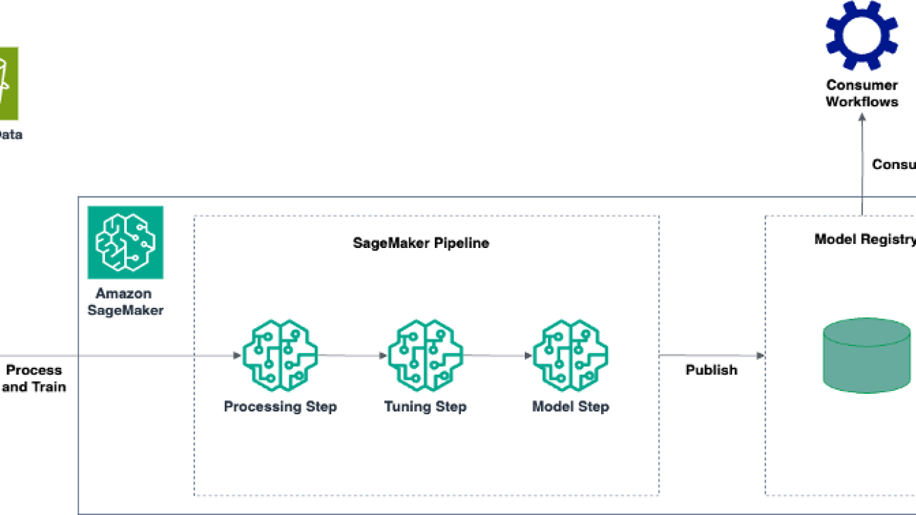
Contemporary log anomaly detection techniques such as Drain-based detection [1] or DeepLog [2] consist of the following general approach: perform custom processing on logs, train their anomaly detection models using custom models, and obtain the best-performing model with an optimal set of hyperparameters. To build an anomaly detection system using such techniques, you need to write custom scripts for processing as well for training. SageMaker provides support for developing scripts by extending in-built algorithm containers, or by building your own custom containers. Moreover, you can combine these steps as a series of interconnected stages using SageMaker Pipelines. The following figure shows an example architecture:

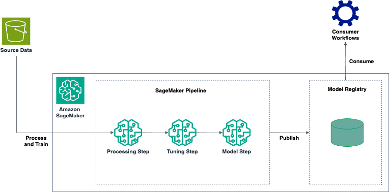
The workflow consists of the following steps:

  1. The log training data is initially stored in an Amazon Simple Storage Service (Amazon S3) bucket, from where it’s picked up by the SageMaker processing step of the SageMaker pipeline.
  2. After the pipeline is started, the processing step loads the Amazon S3 data into SageMaker containers and runs custom processing scripts that parse and process the logs before uploading them to a specified Amazon S3 destination. This processing could be either decentralized with a single script running on one or more instances, or it could be run in parallel over multiple instances using a distributed framework like Apache Spark. We discuss both approaches in this post.
  3. After processing, the data is automatically picked up by the SageMaker tuning step, where multiple training iterations with unique hyperparameter combinations are run for the custom training script.
  4. Finally, the SageMaker model step creates a SageMaker model using the best-trained model obtained from the tuning step and registers it to the SageMaker Model Registry for consumers to use. These consumers, for example, could be testers, who use models trained on different datasets by different pipelines to compare their effectiveness and generality, before deploying them to a public endpoint.

We walk through implementing the solution with the following high-level steps:

  1. Perform custom data processing, using either a decentralized or distributed approach.
  2. Write custom SageMaker training scripts that automatically tune the resulting models with a range of hyperparameters.
  3. Select the best-tuned model, create a custom SageMaker model from it, and register it to the SageMaker Model Registry.
  4. Combine all the steps in a SageMaker pipeline and run it.

Prerequisites

You should have the following prerequisites:

Process the data

To start, upload the log dataset to an S3 bucket in your AWS account. You can use the AWS Command Line Interface (AWS CLI) using Amazon S3 commands, or use the AWS Management Console. To process the data, you use a SageMaker processing step as the first stage in your SageMaker pipeline. This step spins up a SageMaker container and runs a script that you provide for custom processing. There are two ways to do this: decentralized or distributed processing. SageMaker provides Processor classes for both approaches. You can choose either approach for your custom processing depending on your use case.

Decentralized processing with ScriptProcessor

In the decentralized approach, a single custom script runs on one or more standalone instances and processes the input data. The SageMaker Python SDK provides the ScriptProcessor class, which you can use to run your custom processing script in a SageMaker processing step. For small datasets, a single instance can usually suffice for performing data processing. Increasing the number of instances is recommended if your dataset is large and can be split into multiple independent components, which can all be processed separately (this can be done using the ShardedByS3Key parameter, which we discuss shortly).

If you have custom dependencies (which can often be the case during R&D processes), you can extend an existing container and customize it with your dependencies before providing it to the ScriptProcessor class. For example, if you’re using the Drain technique, you need the logparser Python library for log parsing, in which case you write a simple Dockerfile that installs it along with the usual Python ML libraries:

FROM python:3.7-slim-buster
RUN pip3 install pandas==0.25.3 scikit-learn==0.21.3 logparser3 boto3
ENV PYTHONUNBUFFERED=TRUE
ENTRYPOINT ["python3"]

You can use a Python SageMaker notebook instance in your AWS account to create such a Dockerfile and save it to an appropriate folder, such as docker. To build a container using this Dockerfile, enter the following code into a main driver program in a Jupyter notebook on your notebook instance:

import boto3
from sagemaker import get_execution_role

region = boto3.session.Session().region_name
role = get_execution_role()
account_id = boto3.client("sts").get_caller_identity().get("Account")
ecr_repository = "sagemaker-processing-my-container"
tag = ":latest"

uri_suffix = "amazonaws.com"
if region in ["cn-north-1", "cn-northwest-1"]:
uri_suffix = "amazonaws.com.cn"
processing_repository_uri = "{}.dkr.ecr.{}.{}/{}".format(
account_id, region, uri_suffix, ecr_repository + tag
)

# Create ECR repository and push docker image
!docker build -t $ecr_repository docker
!$(aws ecr get-login --region $region --registry-ids $account_id --no-include-email)
!aws ecr create-repository --repository-name $ecr_repository
!docker tag {ecr_repository + tag} $processing_repository_uri
!docker push $processing_repository_uri

This code creates an Amazon Elastic Container Registry (Amazon ECR) repository where your custom container image will be stored (the repository will be created if it’s not already present). The container image is then built, tagged with the repository name (and :latest), and pushed to the ECR repository.

The next step is writing your actual processing script. For more information on writing a processing script using ScriptProcessor, refer to Amazon SageMaker Processing – Fully Managed Data Processing and Model Evaluation. The following are a few key points to remember:

  • A SageMaker processing step loads the data from an input location (Amazon S3 or local developer workspace) to an input path specified by you under the /opt/ml/processing directory of your container. It then runs your script in the container and uploads the output data from your specified path under /opt/ml/processing to an Amazon S3 destination you’ve specified.
  • Customer log datasets can sometimes consist of multiple subsets without any inter-dependencies amongst them. For these cases, you can parallelize your processing by making your processing script run over multiple instances in a single processing step, with each instance processing one of these independent subsets. It’s a good practice to keep the script’s logic redundant so that each execution on every instance happens independently of the others. This avoids duplicative work.

When your script is ready, you can instantiate the SageMaker ScriptProcessor class for running it on your custom container (created in the previous step) by adding the following code to your driver program:

from sagemaker.processing import (
ProcessingInput,
ProcessingOutput,
ScriptProcessor,
)
from sagemaker.workflow.pipeline_context import PipelineSession

from sagemaker.workflow.steps import ProcessingStep

pipeline_session = PipelineSession()
script_processor = ScriptProcessor(
command=["python3"],
image_uri=processing_repository_uri,
role=role,
instance_count=1,
instance_type="ml.m5.xlarge",
sagemaker_session=pipeline_session,
)

script_processor_run_args = script_processor.run(
code="preprocessing.py",
inputs=[ProcessingInput(source="s3://amzn-s3-demo-bucket-pca-detect/processing_input/", destination="/opt/ml/processing/input")],
outputs=[ProcessingOutput(output_name="training", source="/opt/ml/processing/train")
])

step_processing = ProcessingStep(

name="PreprocessStep",

step_args=script_processor_run_args,

)

In the preceding code, a ScriptProcessor class is being instantiated to run the python3 command for running your custom Python script. You provide the following information:

  • You provide the ECR URI of your custom container image and give SageMaker PipelineSession credentials to the class. When you specify the PipelineSession, the ScriptProcessor doesn’t actually begin the execution when you call its run() method—rather, it defers until the SageMaker pipeline as a whole is invoked.
  • In the run() method, you specify the preprocessing script along with the appropriate ProcessingInput and ProcessingOutput These specify where the data will be mounted in your custom container from Amazon S3, and where it will be later uploaded in Amazon S3 from your container’s output folder. The output channel is named training, and the final Amazon output location will be located at s3://<amzn-s3-demo-bucket-pca-detect>/<job-name>/output/<output-name>.

You can also specify an additional parameter in run() named distribution, and it can either be ShardedByS3Key or FullyReplicated, depending on whether you’re splitting and sending your S3 dataset to multiple ScriptProcessor instances or not. You can specify the number of instances in the instance_count parameter of your ScriptProcessor class.

Once instantiated, you can pass the ScriptProcessor class as an argument to the SageMaker processing step along with an appropriate name.

Distributed processing with PySparkProcessor

An alternative to the decentralized processing is distributed processing. Distributed processing is particularly effective when you need to process large amounts of log data. Apache Spark is a popular engine for distributed data processing. It uses in-memory caching and optimized query execution for fast analytic queries against datasets of all sizes. SageMaker provides the PySparkProcessor class within the SageMaker Python SDK for running Spark jobs. For an example of performing distributed processing with PySparkProcessor on SageMaker processing, see Distributed Data Processing using Apache Spark and SageMaker Processing. The following are a few key points to note:

  • To install custom dependencies in your Spark container, you can either build a custom container image (similar to the decentralized processing example) or use the subprocess Python module to install them using pip at runtime. For example, to run the anomaly detection technique on Spark, you need an argformat module, which you can install along with other dependencies as follows:
import subprocess
subprocess.run(["pip3", "install", "scipy", "scikit-learn", "logparser3"])
  • Spark transformations are powerful operations to process your data, and Spark actions are the operations that actually perform the requested transformations on your data. The collect() method is a Spark action that brings all the data from worker nodes to the main driver node. It’s a good practice to use it in conjunction with filter functions so you don’t run into memory issues when working with large log datasets.
  • You should also try to partition your input data based on the total number of cores you plan to have in your SageMaker cluster. The official Spark recommendation is to have approximately 2–3 times the number of partitions as the total number of cores in your cluster.

When your Spark processing script is ready, you can instantiate the SageMaker PySparkProcessor class for running it by adding the following lines to your driver program:

from sagemaker.processing import (
ProcessingInput,
ProcessingOutput,

PySparkProcessor
)

from sagemaker.workflow.steps import ProcessingStep

pipeline_session = PipelineSession()

spark_processor = PySparkProcessor(

base_job_name="hdfs-spark-job",

framework_version="3.1",

role=role,

sagemaker_session=pipeline_session,

instance_count=3,

instance_type="ml.m5.xlarge",

max_runtime_in_seconds=6000,

)

spark_processor.run(

submit_app="./sagemaker_spark_processing.py",

spark_event_logs_s3_uri="s3://amzn-s3-demo-bucket-pca-detect/logs/spark_event_logs",

logs=True,

)

step_processing = ProcessingStep(

name="SparkPreprocessStep",

step_args=spark_processor_run_args,

)

The preceding code instantiates a PySparkProcessor instance with three nodes in the SageMaker cluster with Spark v3.1 installed in them. You submit your Spark processing code to it along with the Amazon S3 location where your event logs would be uploaded. These logs can be useful for debugging.

In the run() method invocation, you don’t need to specify your inputs and outputs, which can be the case if these are fixed Amazon S3 destinations already known to your processing code. Otherwise, you can specify them using the ProcessingInput and ProcessingOutput parameters just like in the decentralized example.

Post-instantiation, the PySparkProcessor class is passed to a SageMaker processing step with an appropriate name. Its execution won’t be triggered until the pipeline is created.

Train and tune the model

Now that your processing steps are complete, you can proceed to the model training step. The training algorithm could either be a classical anomaly detection model like Drain-based detection or a neural-network based model like DeepLog. Every model takes in certain hyperparameters that influence how the model is trained. To obtain the best-performing model, the model is usually executed and validated multiple times over a wide range of hyperparameters. This can be a time-consuming manual process and can instead be automated using SageMaker hyperparameter tuning jobs. Tuning jobs perform hyperparameter optimization by running your training script with a specified range of hyperparameter values and obtaining the best model based on the metrics you specify. You can predefine these metrics if you use built-in SageMaker algorithms or define them for your custom training algorithm.

You first need to write your training script for your anomaly detection model. Keep the following in mind:

  • SageMaker makes artifacts available to your container under the /opt/ml container directory. You should use this when fetching your artifacts. For more details on the SageMaker container structure, see SageMaker AI Toolkits Containers Structure.
  • For using a tuning job, you need to make sure that your code doesn’t hardcode parameter hyperparameter values but instead reads them from the /opt/ml/input/config/hyperparameters.json file in your container where SageMaker places it.
  • When using a custom training script, you also need to add a custom training metric to your script that can be used by the tuning job to find the best model. For this, you should print your desired metrics in your training script using a logger or print function. For example, you could print out custom_metric_value: 91, which indicates that your custom metric’s value is 91. We demonstrate later in this post how SageMaker can be informed about this metric.

When your training script is ready, you can use it inside a SageMaker container. SageMaker provides a wide range of built-in algorithm containers that you can use to run your training code. However, there might be cases when you need to build your own training containers. This could be the case when you need custom libraries installed or if you plan to use a new algorithm not built in by SageMaker. In such a case, you can build your own containers in two ways:

After you create your training container image, you need to define the hyperparameter ranges for your tuning job. For example, if you’re using a custom adaptation of the PCA algorithm (like in Drain-based detection), you add the following lines to your driver program:

from sagemaker.tuner import (

IntegerParameter,

)

hyperparameter_ranges = {
"max_components": IntegerParameter(1, 30, scaling_type="Auto")
}

The preceding code indicates that your hyperparameter max_components is an integer and it ranges from 1–30. The auto scaling type indicates that SageMaker will choose the best scale for hyperparameter changes. For more details on other scaling options, see Hyperparameter scaling types.

Then you can use the following code to fully configure your training and tuning steps in the driver program:

estimator = Estimator(
image_uri= training_image_uri,
role=role,
base_job_name='new_training_job',
sagemaker_session=pipeline_session,
instance_count=1,
instance_type='ml.m5.large',
output_path='s3://amzn-s3-demo-bucket-pca-detect/models/',
metric_definitions=[{'Name': custom_metric, 'Regex': "custom_metric_value: ([0-9\.]+)"}]
)

parameter_tuner = HyperparameterTuner(
estimator,
objective_metric_name ="custom_metric",
hyperparameter_ranges,
metric_definitions=[{'Name': custom_metric, 'Regex': "custom_metric_value: ([0-9\.]+)"}],
max_jobs=30,
max_parallel_jobs=5,
strategy="Bayesian",
objective_type="Maximize",
early_stopping_type="Auto"
)

hpo_args = parameter_tuner.fit(
inputs={
"training": TrainingInput(
s3_data= step_processing.properties.ProcessingOutputConfig.Outputs["training"].S3Output.S3Uri,
s3_data_type="S3Prefix",
distribution="FullyReplicated"
)
}
)

step_tuning = TuningStep(
name="AnomalyDetectionTuning",
step_args=hpo_args,
)

In the preceding code, a SageMaker Estimator instance is created using your custom training image’s ECR URI. SageMaker Estimators help in training your models and orchestrating their training lifecycles. The Estimator is provided with a suitable role and the PipelineSession is designated as its SageMaker session.

You provide the location where your trained model should be stored to the Estimator and supply it with custom metric definitions that you created. For the example metric custom_metric_value: 91, the definition to the Estimator includes its name along with its regex. The regex informs SageMaker how to pick up the metric’s values from training logs in Amazon CloudWatch. The tuning job uses these values to find the best-performing model. You also specify where the output model should be uploaded in the output_path parameter.

You then use this Estimator to instantiate your HyperparameterTuner. Its parameters include the total and maximum parallel number of training jobs, search strategy (for more details on strategies, see Understand the hyperparameter tuning strategies available in Amazon SageMaker AI), and whether you want to use early stopping. Early stopping can be set to Auto so that SageMaker automatically stops model training when it doesn’t see improvements in your custom logged metric.

After the HyperparameterTuner is instantiated, you can call its fit() method. In its input parameter, you specify the output Amazon S3 URI from the processing step as the input location for obtaining training data in your tuning step. This way, you don’t need to specify the Amazon S3 URI yourself and it’s passed between steps implicitly. You can then specify your s3prefix and distribution depending on whether you’re using multiple instances or not.

Once instantiated, the HyperparameterTuner is passed to the tuning step, where it becomes part of your SageMaker pipeline. The training configuration is now complete!

Register the model

You can now choose the best model from the tuning step to create a SageMaker model and publish it to the SageMaker Model Registry. You can use the following driver program code:

from sagemaker import PipelineModel
from sagemaker.workflow.model_step import ModelStep

best_model = sagemaker.model.Model(
image_uri=training_image_uri,
model_data=step_tuning.get_top_model_s3_uri(
top_k=0,
s3_bucket="amzn-s3-demo-bucket-pca-detect",
prefix="models"
)
)

pipeline_model = PipelineModel(
models=[best_model],
role=role,

sagemaker_session=pipeline_session,
)

register_model_step_args = pipeline_model.register(
content_types=["text/csv"],
response_types=["text/csv"],
model_package_group_name="PCAAnomalyDetection",
)

step_model_registration = ModelStep(
name="NewRegistry",
step_args=register_model_step_args,
)

The code instantiates a SageMaker model using the Amazon S3 URI of the best model obtained from the tuning step. The top_k attribute of the get_top_model_s3_uri() method indicates that you’re interested in only obtaining the best-trained model.

After the model is instantiated, you can use it to create a SageMaker PipelineModel so that your pipeline can work directly with your model. You then call the register() method of PipelineModel to register your model to the SageMaker Model Registry. In the register() call, you specify the name of the new model package group where your model will be registered and specify its input and output request and response prediction types.

Finally, a SageMaker ModelStep is invoked with the instantiated PipelineModel to carry out the model registration process.

Create and run a pipeline

You’ve now reached the final step where all your steps will be tied together in a SageMaker pipeline. Add the following code to your driver program to complete your pipeline creation steps:

from sagemaker.workflow.pipeline import Pipeline

pipeline = Pipeline(
name="Anomaly-Detection-Pipeline",
steps=[
step_processing,

step_tuning,
step_model_registration
],
sagemaker_session=pipeline_session,
)
pipeline.upsert(role_arn=role)

pipeline.start()

This code instantiates the SageMaker Pipeline construct and provides it with all the steps defined until now—processing, tuning, and registering the model. It’s provided with a role and then invoked with the start() method.

The pipeline invocation could be on-demand using code (using pipeline.start() as shown earlier) or it could be event-driven using Amazon EventBridge rules. For example, you can create an EventBridge rule that triggers when new training data is uploaded to your S3 buckets and specify your SageMaker pipeline as the target for this rule. This makes sure that when new data is uploaded to your training bucket, your SageMaker pipeline is automatically invoked. For more details on SageMaker and EventBridge integration, refer to Schedule Pipeline Runs.

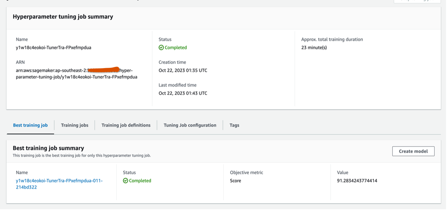
On invocation, your SageMaker pipeline runs your custom processing script in the processing step and uploads the processed data to your specified Amazon S3 destination. It then starts a tuning job with your custom training code and iteratively trains multiple models with your supplied hyperparameters and selects the best model based on your custom provided metric. The following screenshot shows that it selected the best model when tuning was complete:

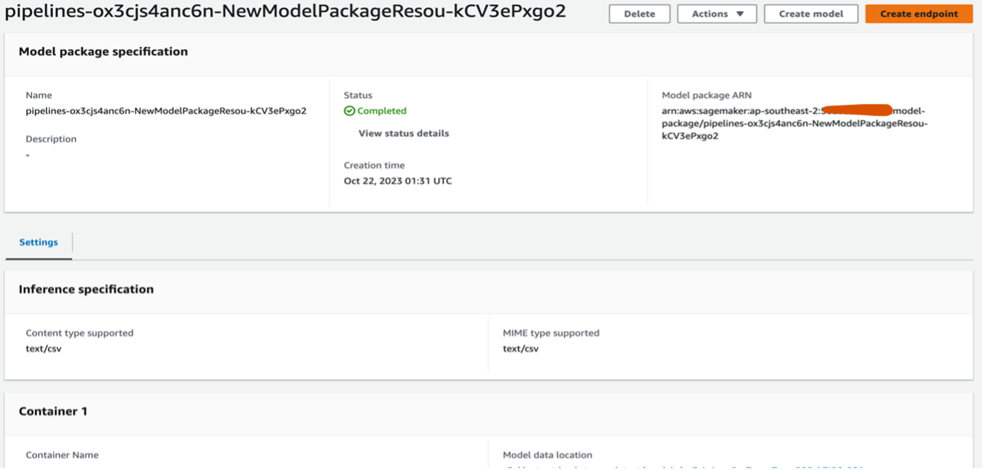
Finally, the best model is selected and a model package resource is created with it in your model registry. Your customers can use it to deploy your model:

You have now completed all the steps in processing, training, tuning, and registering your custom anomaly detection model automatically with the aid of a SageMaker pipeline that was initiated using your driver program.

Clean up

To avoid incurring future charges, complete the following steps:

  1. Delete the SageMaker notebook instance used for this post.
  2. Delete the model package resource that was created using the best-tuned model.
  3. Delete any Amazon S3 data that was used for this post.

Conclusion

In this post, we demonstrated the building, training, tuning, and registering of an anomaly detection system with custom processing code, custom training code, and custom training metrics. We ran these steps automatically with the aid of a SageMaker pipeline, which was run by invoking a single main driver program. We also discussed the different ways of processing our data, and how it could be done using the various constructs and tools that SageMaker provides in a user-friendly and straightforward manner.

Try this approach for building your own custom anomaly detection model, and share your feedback in the comments.

References

[1] https://ieeexplore.ieee.org/document/8029742

[2] https://dl.acm.org/doi/pdf/10.1145/3133956.3134015


About the Author

Nitesh Sehwani is an SDE with the EC2 Threat Detection team where he’s involved in building large-scale systems that provide security to our customers. In his free time, he reads about art history and enjoys listening to mystery thrillers.

Read More

High-Performance Low-Bit Operators for PyTorch

High-Performance Low-Bit Operators for PyTorch

We are excited to announce the addition of embedding operators with low-bit weights (1-8 bit) and linear operators with 8-bit dynamically quantized activations and low-bit weights (1-8 bit) for Arm CPUs in TorchAO, PyTorch’s native low-precision library. These operators work seamlessly across all PyTorch surfaces, including eager, torch.compile, AOTI, and ExecuTorch, and are available to use in torchchat.

In developing these linear operators, our focus was on code sharing between PyTorch and ExecuTorch, and establishing a clear boundary between the higher-level operator and the lower-level kernel. This design allows third-party vendors to easily swap in their own kernels. We also set out to create a place and infrastructure to experiment with new CPU quantization ideas and test those across the PyTorch ecosystem.

Universal low-bit kernels

There is no hardware support for low-bit arithmetic. In what we call universal kernels, we explicitly separated the logic that unpacks low-bit values to int8 values, and the int8 GEMV kernel logic in a modular fashion. We started with an 8-bit kernel, for example, this 1×8 8-bit GEMV kernel that uses the Arm neondot instruction. Within the 8-bit kernel, we invoke an inlined unpacking routine to convert low-bit values into int8 values. This unpacking routine is force-inlined and templated on some low-bit value. Our experiments showed no performance difference between using a separate force-inlined unpacking routine and directly embedding the unpacking code inline.

The advantage of this modular design is improved development speed and code maintainability. After writing an 8-bit kernel, we quickly achieved full low-bit coverage by writing simple bitpacking routines. In fact, developers who worked on the bit packing routines did not need to be experts on GEMV/GEMM kernel writing. We also reused the same bitpacking routines from the linear kernels within the embedding kernels. In future we could reuse the same bitpacking routines for universal GEMM kernels or kernels based on fma or i8mm instructions.

Shared code between PyTorch and ExecuTorch

To achieve shared code between PyTorch and ExecuTorch, we wrote kernels using raw pointers instead of PyTorch tensors. Moreover, we implemented the linear operator in a header that is included in separate PyTorch and ExecuTorch operator registration code. By using only features common to both ATen and ExecuTorch tensors, we ensured compatibility between the two frameworks. For multi-threaded compute, we introduced torchao::parallel_1d, which compiles to either at::parallel_for or ExecuTorch’s threadpool based on compile-time flags.

Swappable kernels

Our design for the higher-level multi-threaded linear operator is agnostic to the lower-level single-threaded kernels, allowing third-party vendors to swap in their own implementations. The interface between the operator and kernel is defined by a ukernel config, which specifies kernel function pointers for preparing activation data, preparing weight data, and running the kernel. The operator, responsible for tiling and scheduling, interacts with kernels solely through this config.

Performance

In the table below, we show Llama3.1 8B token generation performance using 6 CPU threads on an M1 Macbook Pro with 32GB of RAM.

Bitwidth x torch.compile (Decode tokens/sec) ExecuTorch (Decode tokens/sec) ExecuTorch PTE size (GiB)
1 24.18 17.86 1.46
2 27.02 19.65 2.46
3 21.01 22.25 3.46
4 19.51 19.47 4.47
5 14.78 16.34 5.47
6 12.80 13.61 6.47
7 8.16 11.73 7.48

Results were run on an M1 Macbook Pro (with 8 perf cores, and 2 efficiency cores) with 32GB of RAM and 6 threads using torchchat. In each test, the max-seq-length of 128 tokens were generated. For each bit width x, the embedding layer was groupwise quantized to x-bits with group size 32. In the linear layers, activations were dynamically quantized per token to 8 bits and weights were groupwise quantized to x-bits with group size 256. Our focus here is performance and we do not report accuracy or perplexity numbers. Depending on the model, lower bit widths may require quantization-aware training, quantizing a model with a mixture of bit widths, or adjusting the group sizes for acceptable accuracy.

Llama 3.1 chart

Try them out and contribute!

If you want to see the new low-bit kernels in action, give them a try by setting up torchchat and quantizing and running an LLM locally using the kernels.

If you want to help contribute, consider adding support for one of the following areas:

  • Add universal low-bit GEMM kernels for Arm CPU, reusing the same bitpacking routines from the universal GEMV kernels.
  • Improve runtime selection of ukernel configs based on ISA, packing format, and activation shape.
  • Add low-bit kernels for other CPU ISAs like x86.
  • Integrate third-party libraries like KleidiAI with the operator framework.

Read More

3D Shape Tokenization

We introduce Shape Tokens, a 3D representation that is continuous, compact, and easy to integrate into machine learning models. Shape Tokens serve as conditioning vectors, representing shape information within a 3D flow-matching model. This flow-matching model is trained to approximate probability density functions corresponding to delta functions concentrated on the surfaces of 3D shapes. By incorporating Shape Tokens into various machine learning models, we can generate new shapes, convert images to 3D, align 3D shapes with text and images, and render shapes directly at variable…Apple Machine Learning Research

How AI Is Helping Us Do Better—for the Planet and for Each Other

How AI Is Helping Us Do Better—for the Planet and for Each Other

Artificial intelligence and accelerated computing are being used to help solve the world’s greatest challenges.

NVIDIA has reinvented the computing stack — spanning GPUs, CPUs, DPUs, networking and software. Our platform drives the AI revolution, powering hundreds of millions of devices in every cloud and fueling 75% of the world’s TOP500 supercomputers.

Put in the hands of entrepreneurs and enterprises, developers and scientists, that platform becomes a system for invention, and a force for good across industries and geographies.

Here are five examples of how these technologies are being put to work from the past year:

Supporting Surgeons

Illinois-based startup SimBioSys has created TumorSight Viz, a technology that converts MRI images into 3D models of breast tissue. This helps surgeons better treat breast cancers by providing detailed visualizations of tumors and surrounding tissue.

Saving Lives and Energy

Researchers at the Wellcome Sanger Institute, a key player in the Human Genome Project, analyze tens of thousands of cancer genomes annually, providing insights into cancer formation and treatment effectiveness. NVIDIA accelerated computing and software drastically reduce the institute’s analysis runtime and energy consumption per genome.

Cleaning Up Our Waters

Clearbot, developed by University of Hong Kong grads, is an AI-driven sea-cleaning boat that autonomously collects trash from the water. Enabled by the NVIDIA Jetson platform, Clearbot is making a splash in Hong Kong and India, helping keep tourist regions clean.

Greening Recycling Plants

Greyparrot, a UK-based startup, has developed the Greyparrot Analyzer, an AI-powered device that offers “waste intelligence” to recycling plants. Using embedded cameras and machine learning, the analyzer identifies and differentiates materials on conveyor belts, significantly improving recycling efficiency.

Driving Technological Advancement in Africa

A new AI innovation hub has launched in Tunisia, part of NVIDIA’s efforts to train 100,000 developers across Africa. Built in collaboration with the NVIDIA Deep Learning Institute, the hub offers training, technologies and business networks to drive AI adoption across the continent.

All of these initiatives — whether equipping surgeons with new tools or making recycling plants greener — rely on the ingenuity of human beings across the globe, humans increasingly supercharged by AI.

Find more examples of how AI is helping people from across industries and the globe to make a difference and drive positive social impact.

Read More

Inductive biases of neural network modularity in spatial navigation

Inductive biases of neural network modularity in spatial navigation

TL;DR: The brain may have evolved a modular architecture for daily tasks, with circuits featuring functionally specialized modules that match the task structure. We hypothesize that this architecture enables better learning and generalization than architectures with less specialized modules. To test this, we trained reinforcement learning agents with various neural architectures on a naturalistic navigation task. We found that the modular agent, with an architecture that segregates computations of state representation, value, and action into specialized modules, achieved better learning and generalization. Our results shed light on the possible rationale for the brain’s modularity and suggest that artificial systems can use this insight from neuroscience to improve learning and generalization in natural tasks.

Motivation

Despite the tremendous success of AI in recent years, it remains true that even when trained on the same data, the brain outperforms AI in many tasks, particularly in terms of fast in-distribution learning and zero-shot generalization to unseen data. In the emerging field of neuroAI (Zador et al., 2023), we are particularly interested in uncovering the principles underlying the brain’s extraordinary capabilities so that these principles can be leveraged to develop more versatile and general-purpose AI systems.

Given the same training data, the differing abilities of learning systems—biological or artificial—stem from their distinct assumptions about the data, known as inductive biases. For instance, if the underlying data distribution is linear, a linear model that assumes linearity can learn very quickly—by observing only a few points without needing to fit the entire dataset—and generalize effectively to unseen data. In contrast, another model with a different assumption, such as quadratic, cannot achieve the same performance. Even if it were a powerful universal function approximator, it would not achieve the same efficiency. The brain may have evolved inductive biases that align with the underlying structure of natural tasks, which explains its high efficiency and generalization abilities in such tasks.

What are the brain’s useful inductive biases? One perspective suggests that the brain may have evolved an inductive bias for a modular architecture featuring functionally specialized modules (Bertolero et al., 2015). Each module specializes in a specific aspect or a subset of task variables, collectively covering all demanding computations of the task. We hypothesize that this architecture enables higher efficiency in learning the structure of natural tasks and better generalization in tasks with a similar structure than those with less specialized modules.

Previous works (Goyal et al., 2022; Mittal et al., 2022) have outlined the potential rationale for this architecture: Data generated from natural tasks typically stem from the latent distribution of multiple task variables. Decomposing the task and learning these variables in distinct modules allow a better understanding of the relationships among these variables and therefore the data generation process. This modularization also promotes hierarchical computation, where independent variables are initially computed and then forwarded to other modules specialized in computing dependent variables. Note that “modular” may take on different meanings in different contexts. Here, it specifically refers to architectures with multiple modules, each specializing in one or a subset of the desired task variables. Architectures with multiple modules lacking enforced specialization in computing variables do not meet the criteria for modular in our context.

To test our hypothesis, it is essential to select a natural task and compare a modular architecture designed for the task with alternative architectures.

Task

We chose a naturalistic virtual navigation task (Figure 1) previously used to investigate the neural computations underlying animals’ flexible behaviors (Lakshminarasimhan et al., 2020). At the beginning of each trial, the subject is situated at the center of the ground plane facing forward; a target is presented at a random location within the field of view (distance: (100) to (400) cm, angle: (-35) to (+35^{circ})) on the ground plane and disappears after (300) ms. The subject can freely control its linear and angular velocities with a joystick (maximum: (200) cm/s and (90^{circ})/s, referred to as the joystick gain) to move along its heading in the virtual environment. The objective is to navigate toward the memorized target location, then stop inside the reward zone, a circular region centered at the target location with a radius of (65) cm. A reward is given only if the subject stops inside the reward zone.

Figure 1

The subject’s self-location is not directly observable because there are no stable landmarks; instead, the subject needs to use optic flow cues on the ground plane to perceive self-motion and perform path integration. Each textural element of the optic flow, an isosceles triangle, appears at random locations and orientations, disappearing after only a short lifetime ((sim 250) ms), making it impossible to use as a stable landmark. A new trial starts after the subject stops moving.

Task modeling

We formulate this task as a Partially Observable Markov Decision Process (POMDP; Kaelbling et al., 1998) in discrete time, with continuous state and action spaces (Figure 2). At each time step (t), the environment is in the state (boldsymbol{s}_t) (including the agent’s position and velocity, and the target’s position). The agent takes an action (boldsymbol{a}_t) (controlling its linear and angular velocities) to update (boldsymbol{s}_t) to the next state (boldsymbol{s}_{t+1}) following the environmental dynamics given by the transition probability (T(boldsymbol{s}_{t+1}|boldsymbol{s}_{t},boldsymbol{a}_{t})), and receives a reward (r_t) from the environment following the reward function (R(boldsymbol{s}_t,boldsymbol{a}_t)) ((1) if the agent stops inside the reward zone otherwise (0)).

We use a model-free actor-critic approach to learning, with the actor and critic implemented using distinct neural networks. At each (t), the actor receives two sources of inputs (boldsymbol{i}_t) about the state: observation (boldsymbol{o}_t) and last action (boldsymbol{a}_{t-1}). It then outputs an action (boldsymbol{a}_t), aiming to maximize the state-action value (Q_t). This value is a function of the state and action, representing the expected discounted rewards when an action is taken at a state, and future rewards are then accumulated from (t) until the trial’s last step. Since the ground truth value is unknown, the critic is used to approximate the value. In addition to receiving the same inputs (boldsymbol{i}_t) as the actor to infer the state, the critic also takes as inputs the action (boldsymbol{a}_t) taken by the actor in this state. It then outputs the estimated (Q_t) for this action, trained through the temporal-difference error (TD error) after receiving the reward (r_t) ((|r_t+gamma Q_{t+1}-Q_{t}|), where (gamma) denotes the temporal discount factor). In practice, our algorithm is off-policy and incorporates mechanisms such as two critic networks and target networks as in TD3 (fujimoto et al., 2018) to enhance training (see Materials and Methods in Zhang et al., 2024).

Figure 2

The state (boldsymbol{s}_t) is not fully observable, so the agent must maintain an internal state representation (belief (b_t)) for deciding (boldsymbol{a}_t) and (Q_t). Both actor and critic undergo end-to-end training through back-propagation without explicit objectives for shaping (b_t). Consequently, networks are free to learn diverse forms of (b_t) encoded in their neural activities that aid them in achieving their learning objectives. Ideally, networks may develop an effective belief update rule, e.g., recursive Bayesian estimation, using the two sources of evidence in the inputs (boldsymbol{i}_t={boldsymbol{o}_t, boldsymbol{a}_{t-1}}). They may predict the state (boldsymbol{s}_t) based on its internal model of the dynamics, its previous belief (b_{t-1}), and the last self-action (boldsymbol{a}_{t-1}). The second source is a partial and noisy observation (boldsymbol{o}_t) of (boldsymbol{s}_t) drawn from the observation probability (O(boldsymbol{o}_t|boldsymbol{s}_t)). Note that the actual (O) in the brain for this task is unknown. For simplicity, we model (boldsymbol{o}_t) as a low-dimensional vector, including the target’s location when visible (the first (300) ms, (Delta t=0.1) s), and the agent’s observation of its velocities through optic flow, with velocities subject to Gaussian additive noise.

Actor-critic RL agent

Each RL agent requires an actor and a critic network, and actor and critic networks can have a variety of architectures. Our goal here is to investigate whether functionally specialized modules provide advantages for our task. Therefore, we designed architectures incorporating modules with distinct levels of specialization for comparison. The first architecture is a holistic actor/critic, comprising a single module where all neurons jointly compute the belief (b_t) and the action (boldsymbol{a}_t)/value (Q_t). In contrast, the second architecture is a modular actor/critic, featuring modules specialized in computing different variables (Figure 3).

Figure 3

The specialization of each module is determined as follows.

First, we can confine the computation of beliefs. Since computing beliefs about the evolving state requires integrating evidence over time, a network capable of computing belief must possess some form of memory. Recurrent neural networks (RNNs) satisfy this requirement by using a hidden state that evolves over time. In contrast, computations of value and action do not need additional memory when the belief is provided, making memoryless multi-layer perceptrons (MLPs) sufficient. Consequently, adopting an architecture with an RNN followed by a memoryless MLP (modular actor/critic in Figure 3) ensures that the computation of belief is exclusively confined to the RNN.

Second, we can confine the computation of the state-action value (Q_t) for the critic. Since a critic is trained end-to-end to compute (Q_t), stacking two modules between all inputs and outputs does not limit the computation of (Q_t) to a specific module. However, since (Q_t) is a function of the action (boldsymbol{a}_t), we can confine the computation of (Q_t) to the second module of the modular critic in Figure 3 by supplying (boldsymbol{a}_t) only to the second module. This ensures that the first module, lacking access to the action, cannot accurately compute (Q_t). Therefore, the modular critic’s RNN is dedicated to computing (b_t) and sends it to the MLP dedicated to computing (Q_t). This architecture enforces modularity.

Besides the critic, the modular actor has higher specialization than the holistic actor, which lacks confined (b_t) computation. Thought bubbles in Figure 3 denote the variables that can be computed within each module enforced through architecture rather than indicating they are encoded in each module. For example, (b_t) in modular architectures is passed to the second module, but an accurate (b_t) computation can only be completed in the first RNN module.

Behavioral accuracy

We trained agents using all four combinations of these two actor and critic architectures. We refer to an agent whose actor and critic are both holistic or both modular as a holistic agent or a modular agent, respectively. Agents with modular critics demonstrated greater consistency across various random seeds and achieved near-perfect accuracy more efficiently than agents with holistic critics (Figure 4).

Figure 4

Agents’ behavior was compared with that of two monkeys (Figure 5 left) for a representative set of targets uniformly sampled on the ground plane (Figure 5 right).

Figure 5

We used a Receiver Operating Characteristic (ROC) analysis (Lakshminarasimhan et al., 2020) to systematically quantify behavioral accuracy. A psychometric curve for stopping accuracy is constructed from a large representative dataset by counting the fraction of rewarded trials as a function of a hypothetical reward boundary size (Figure 6 left, solid; radius (65) cm is the true size; infinitely small/large reward boundary leads to no/all rewarded trials). A shuffled curve is constructed similarly after shuffling targets across trials (Figure 6 left, dashed). Then, an ROC curve is obtained by plotting the psychometric curve against the shuffled curve (Figure 6 right). An ROC curve with a slope of (1) denotes a chance level (true(=)shuffled) with the area under the curve (AUC) equal to (0.5). High AUC values indicate that all agents reached good accuracy after training (Figure 6 right, inset).

Figure 6

Although all agents exhibited high stop location accuracy, we have noticed distinct characteristics in their trajectories (Figure 5 left). To quantify these differences, we examined two crucial trajectory properties: curvature and length. When tested on the same series of targets as the monkeys experienced, the difference between trajectories generated by agents with modular critics and those of monkey B was comparable to the variation between trajectories of two monkeys (Figure 7). In contrast, when agents used holistic critics, the difference in trajectories from monkey B was much larger, suggesting that modular critics facilitated more animal-like behaviors.

Figure 7

Behavioral efficiency

Agents are expected to develop efficient behaviors, as the value of their actions gets discounted over time. Therefore, we assess their efficiency throughout the training process by measuring the reward rate, which refers to the number of rewarded trials per second. We found that agents with modular critics achieved much higher reward rates, which explains their more animal-like efficient trajectories (Figure 8).

Figure 8

Together, these results suggest that modular critics provide a superior training signal compared to holistic critics, allowing actors to learn more optimal beliefs and actions. With a poor training signal from the holistic critic, the modularization of actors may not enhance performance. Next, we will evaluate the generalization capabilities of the trained agents.

An unseen task

One crucial aspect of sensorimotor mapping is the joystick gain, which linearly maps motor actions on the joystick (dimensionless, bounded in ([-1,1])) to corresponding velocities in the environment. During training, the gain remains fixed at (200) cm/s and (90^{circ})/s for linear and angular components, referred to as the (1times) gain. By increasing the gain to values that were not previously experienced, we create a gain task manipulation.

To assess generalization abilities, monkeys and agents were tested with novel gains of (1.5times) and (2times) (Figure 9).

Figure 9

Blindly following the same action sequence as in the training task would cause the agents to overshoot (no-generalization hypothesis: Figure 10 dashed lines). Instead, the agents displayed varying degrees of adaptive behavior (Figure 10 solid lines).

Figure 10

To quantitatively evaluate behavioral accuracy while also considering over-/under-shooting effects, we defined radial error as the Euclidean distance between the stop and target locations in each trial, with positive/negative sign denoting over-/under-shooting. Under the novel gains, agents with modular critics consistently exhibited smaller radial errors than agents with holistic critics (Figure 11), with the modular agent demonstrating the smallest errors, comparable to those observed in monkeys.

Figure 11

Neural analysis

Although we have confirmed that agents with distinct neural architectures exhibit varying levels of generalization in the gain task, the underlying mechanism remains unclear. We hypothesized that agents with superior generalization abilities should generate actions based on more accurate internal beliefs within their actor networks. Therefore, the goal next is to quantify the accuracy of beliefs across agents tested on novel gains, and to examine the impact of this accuracy on their generalization performance.

During the gain task, we recorded the activities of RNN neurons in the agents’ actors, as these neurons are responsible for computing the beliefs that underlie actions. To systematically quantify the accuracy of these beliefs, we used linear regression (with (ell_2) regularization) to decode agents’ locations from the recorded RNN activities for each gain condition (Figure 12).

Figure 12

We defined the decoding error, which represents the Euclidean distance between the true and decoded locations, as an indicator of belief accuracy. While all agents demonstrated small decoding errors under the training gain, we found that more holistic agents struggling with generalization under increased gains also displayed reduced accuracy in determining their own location (Figure 13 left). In fact, agents’ behavioral performance correlates with their belief accuracy (Figure 13 right).

Figure 13

Conclusion

The brain has evolved advantageous modular architectures for mastering daily tasks. Here, we investigated the impact of architectural inductive biases on learning and generalization using deep RL agents. We posited that an architecture with functionally specialized modules would allow agents to more efficiently learn essential task variables and their dependencies during training, and then use this knowledge to support generalization in novel tasks with a similar structure. To test this, we trained agents with architectures featuring distinct module specializations on a partially observable navigation task. We found that the agent using a modular architecture exhibited superior learning of belief and control actions compared to agents with weaker modular specialization.

Furthermore, for readers interested in the full paper, we also demonstrated that the modular agent’s beliefs closely resemble an Extended Kalman Filter, appropriately weighting information sources based on their relative reliability. Additionally, we presented several more architectures with varying levels of modularity and confirmed that greater modularity leads to better performance.

Read More