Monthly Archives: January 2025

Generative AI and large language models (LLMs) are revolutionizing organizations across diverse sectors to enhance customer experience, which traditionally would take years to make progress. Every organization has data stored in data stores, either on premises or in cloud providers.

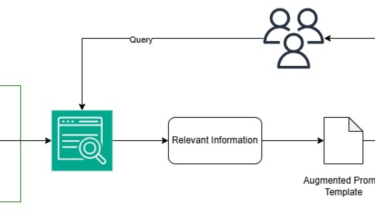
You can embrace generative AI and enhance customer experience by converting your existing data into an index on which generative AI can search. When you ask a question to an open source LLM, you get publicly available information as a response. Although this is helpful, generative AI can help you understand your data along with additional context from LLMs. This is achieved through Retrieval Augmented Generation (RAG).

RAG retrieves data from a preexisting knowledge base (your data), combines it with the LLM’s knowledge, and generates responses with more human-like language. However, in order for generative AI to understand your data, some amount of data preparation is required, which involves a big learning curve.

Amazon Aurora is a MySQL and PostgreSQL-compatible relational database built for the cloud. Aurora combines the performance and availability of traditional enterprise databases with the simplicity and cost-effectiveness of open source databases.

In this post, we walk you through how to convert your existing Aurora data into an index without needing data preparation for Amazon Kendra to perform data search and implement RAG that combines your data along with LLM knowledge to produce accurate responses.

Solution overview

In this solution, use your existing data as a data source (Aurora), create an intelligent search service by connecting and syncing your data source to Amazon Kendra search, and perform generative AI data search, which uses RAG to produce accurate responses by combining your data along with the LLM’s knowledge. For this post, we use Anthropic’s Claude on Amazon Bedrock as our LLM.

The following are the high-level steps for the solution:

• Create an Amazon Aurora PostgreSQL-Compatible Edition
• Ingest data to Aurora PostgreSQL-Compatible.
• Create an Amazon Kendra index.
• Set up the Amazon Kendra Aurora PostgreSQL connector.
• Invoke the RAG application.

The following diagram illustrates the solution architecture.

Prerequisites

To follow this post, the following prerequisites are required:

• The AWS Command Line Interface (AWS CLI) installed and configured
• An AWS account and appropriate permissions to interact with resources in your AWS account
• The AWS managed AWS Identity and Access Management (IAM) policy AmazonKendraReadOnlyAccess should be part of an Amazon SageMaker IAM role
• An Aurora DB cluster where the current data is present
• Your preferred interactive development environment (IDE) to run the Python script (such as SageMaker, or VS Code)
• The pgAdmin tool for data loading and validation

Create an Aurora PostgreSQL cluster

Run the following AWS CLI commands to create an Aurora PostgreSQL Serverless v2 cluster:

aws rds create-db-cluster 
--engine aurora-postgresql 
--engine-version 15.4 
--db-cluster-identifier genai-kendra-ragdb 
--master-username postgres 
--master-user-password XXXXX 
--db-subnet-group-name dbsubnet 
--vpc-security-group-ids "sg-XXXXX" 
--serverless-v2-scaling-configuration "MinCapacity=2,MaxCapacity=64" 
--enable-http-endpoint 
--region us-east-2

aws rds create-db-instance 
--db-cluster-identifier genai-kendra-ragdb 
--db-instance-identifier genai-kendra-ragdb-instance 
--db-instance-class db.serverless 
--engine aurora-postgresql

The following screenshot shows the created instance.

Ingest data to Aurora PostgreSQL-Compatible

Connect to the Aurora instance using the pgAdmin tool. Refer to Connecting to a DB instance running the PostgreSQL database engine for more information. To ingest your data, complete the following steps:

1. Run the following PostgreSQL statements in pgAdmin to create the database, schema, and table:

   CREATE DATABASE genai;
   CREATE SCHEMA 'employees';
   
   CREATE DATABASE genai;
   SET SCHEMA 'employees';
   
   CREATE TABLE employees.amazon_review(
   pk int GENERATED ALWAYS AS IDENTITY NOT NULL,
   id varchar(50) NOT NULL,
   name varchar(300) NULL,
   asins Text NULL,
   brand Text NULL,
   categories Text NULL,
   keys Text NULL,
   manufacturer Text NULL,
   reviews_date Text NULL,
   reviews_dateAdded Text NULL,
   reviews_dateSeen Text NULL,
   reviews_didPurchase Text NULL,
   reviews_doRecommend varchar(100) NULL,
   reviews_id varchar(150) NULL,
   reviews_numHelpful varchar(150) NULL,
   reviews_rating varchar(150) NULL,
   reviews_sourceURLs Text NULL,
   reviews_text Text NULL,
   reviews_title Text NULL,
   reviews_userCity varchar(100) NULL,
   reviews_userProvince varchar(100) NULL,
   reviews_username Text NULL,
   PRIMARY KEY
   (
   pk
   )
   ) ;

2. In your pgAdmin Aurora PostgreSQL connection, navigate to Databases, genai, Schemas, employees, Tables.
3. Choose (right-click) Tables and choose PSQL Tool to open a PSQL client connection.
   
4. Place the csv file under your pgAdmin location and run the following command:

   copy employees.amazon_review (id, name, asins, brand, categories, keys, manufacturer, reviews_date, reviews_dateadded, reviews_dateseen, reviews_didpurchase, reviews_dorecommend, reviews_id, reviews_numhelpful, reviews_rating, reviews_sour
   ceurls, reviews_text, reviews_title, reviews_usercity, reviews_userprovince, reviews_username) FROM 'C:Program FilespgAdmin 4runtimeamazon_review.csv' DELIMITER ',' CSV HEADER ENCODING 'utf8';

   

5. Run the following PSQL query to verify the number of records copied:

   Select count (*) from employees.amazon_review;

   

Create an Amazon Kendra index

The Amazon Kendra index holds the contents of your documents and is structured in a way to make the documents searchable. It has three index types:

• Generative AI Enterprise Edition index – Offers the highest accuracy for the Retrieve API operation and for RAG use cases (recommended)
• Enterprise Edition index – Provides semantic search capabilities and offers a high-availability service that is suitable for production workloads
• Developer Edition index – Provides semantic search capabilities for you to test your use cases

To create an Amazon Kendra index, complete the following steps:

1. On the Amazon Kendra console, choose Indexes in the navigation pane.
2. Choose Create an index.
3. On the Specify index details page, provide the following information:
   • For Index name, enter a name (for example, genai-kendra-index).
   • For IAM role, choose Create a new role (Recommended).
   • For Role name, enter an IAM role name (for example, genai-kendra). Your role name will be prefixed with AmazonKendra-<region>- (for example, AmazonKendra-us-east-2-genai-kendra).
4. Choose Next.
   
5. On the Add additional capacity page, select Developer edition (for this demo) and choose Next.
   
6. On the Configure user access control page, provide the following information:
   • Under Access control settings¸ select No.
   • Under User-group expansion, select None.
7. Choose Next.
   
8. On the Review and create page, verify the details and choose Create.
   

It might take some time for the index to create. Check the list of indexes to watch the progress of creating your index. When the status of the index is ACTIVE, your index is ready to use.

Set up the Amazon Kendra Aurora PostgreSQL connector

Complete the following steps to set up your data source connector:

1. On the Amazon Kendra console, choose Data sources in the navigation pane.
2. Choose Add data source.
3. Choose Aurora PostgreSQL connector as the data source type.
   
4. On the Specify data source details page, provide the following information:
   • For Data source name, enter a name (for example, data_source_genai_kendra_postgresql).
   • For Default language¸ choose English (en).
   • Choose Next.
     
5. On the Define access and security page, under Source, provide the following information:
   • For Host, enter the host name of the PostgreSQL instance (cvgupdj47zsh.us-east-2.rds.amazonaws.com).
   • For Port, enter the port number of the PostgreSQL instance (5432).
   • For Instance, enter the database name of the PostgreSQL instance (genai).
     
6. Under Authentication, if you already have credentials stored in AWS Secrets Manager, choose it on the dropdown Otherwise, choose Create and add new secret.
7. In the Create an AWS Secrets Manager secret pop-up window, provide the following information:
   • For Secret name, enter a name (for example, AmazonKendra-Aurora-PostgreSQL-genai-kendra-secret).
   • For Data base user name, enter the name of your database user.
   • For Password¸ enter the user password.
8. Choose Add Secret.
   
9. Under Configure VPC and security group, provide the following information:
   • For Virtual Private Cloud, choose your virtual private cloud (VPC).
   • For Subnet, choose your subnet.
   • For VPC security groups, choose the VPC security group to allow access to your data source.
10. Under IAM role¸ if you have an existing role, choose it on the dropdown menu. Otherwise, choose Create a new role.
    
11. On the Configure sync settings page, under Sync scope, provide the following information:
    • For SQL query, enter the SQL query and column values as follows: select * from employees.amazon_review.
    • For Primary key, enter the primary key column (pk).
    • For Title, enter the title column that provides the name of the document title within your database table (reviews_title).
    • For Body, enter the body column on which your Amazon Kendra search will happen (reviews_text).
12. Under Sync node, select Full sync to convert the entire table data into a searchable index.

After the sync completes successfully, your Amazon Kendra index will contain the data from the specified Aurora PostgreSQL table. You can then use this index for intelligent search and RAG applications.

13. Under Sync run schedule, choose Run on demand.
14. Choose Next.
    
15. On the Set field mappings page, leave the default settings and choose Next.
    
16. Review your settings and choose Add data source.
    

Your data source will appear on the Data sources page after the data source has been created successfully.

Invoke the RAG application

The Amazon Kendra index sync can take minutes to hours depending on the volume of your data. When the sync completes without error, you are ready to develop your RAG solution in your preferred IDE. Complete the following steps:

1. Configure your AWS credentials to allow Boto3 to interact with AWS services. You can do this by setting the AWS_ACCESS_KEY_ID and AWS_SECRET_ACCESS_KEY environment variables or by using the ~/.aws/credentials file:

   import boto3
     pip install langchain
   
   # Create a Boto3 session
   
   session = boto3.Session(
      aws_access_key_id='YOUR_AWS_ACCESS_KEY_ID',
      aws_secret_access_key='YOUR_AWS_SECRET_ACCESS_KEY',
      region_name='YOUR_AWS_REGION'
   )

2. Import LangChain and the necessary components:

   from langchain_community.llms import Bedrock
   from langchain_community.retrievers import AmazonKendraRetriever
   from langchain.chains import RetrievalQA

3. Create an instance of the LLM (Anthropic’s Claude):

   llm = Bedrock(
   region_name = "bedrock_region_name",
   model_kwargs = {
   "max_tokens_to_sample":300,
   "temperature":1,
   "top_k":250,
   "top_p":0.999,
   "anthropic_version":"bedrock-2023-05-31"
   },
   model_id = "anthropic.claude-v2"
   )

4. Create your prompt template, which provides instructions for the LLM:

   from langchain_core.prompts import PromptTemplate
   
   prompt_template = """
   You are a <persona>Product Review Specialist</persona>, and you provide detail product review insights.
   You have access to the product reviews in the <context> XML tags below and nothing else.
   
   <context>
   {context}
   </context>
   
   <question>
   {question}
   </question>
   """
   
   prompt = PromptTemplate(template=prompt_template, input_variables=["context", "question"])

5. Initialize the KendraRetriever with your Amazon Kendra index ID by replacing the Kendra_index_id that you created earlier and the Amazon Kendra client:

   session = boto3.Session(region_name='Kendra_region_name')
   kendra_client = session.client('kendra')
   # Create an instance of AmazonKendraRetriever
   kendra_retriever = AmazonKendraRetriever(
   kendra_client=kendra_client,
   index_id="Kendra_Index_ID"
   )

6. Combine Anthropic’s Claude and the Amazon Kendra retriever into a RetrievalQA chain:

   qa = RetrievalQA.from_chain_type(
   llm=llm,
   chain_type="stuff",
   retriever=kendra_retriever,
   return_source_documents=True,
   chain_type_kwargs={"prompt": prompt},
   )

7. Invoke the chain with your own query:

   query = "What are some products that has bad quality reviews, summarize the reviews"
   result_ = qa.invoke(
   query
   )
   result_

   

Clean up

To avoid incurring future charges, delete the resources you created as part of this post:

1. Delete the Aurora DB cluster and DB instance.
2. Delete the Amazon Kendra index.

Conclusion

In this post, we discussed how to convert your existing Aurora data into an Amazon Kendra index and implement a RAG-based solution for the data search. This solution drastically reduces the data preparation need for Amazon Kendra search. It also increases the speed of generative AI application development by reducing the learning curve behind data preparation.

Try out the solution, and if you have any comments or questions, leave them in the comments section.

About the Authors

Aravind Hariharaputran is a Data Consultant with the Professional Services team at Amazon Web Services. He is passionate about Data and AIML in general with extensive experience managing Database technologies .He helps customers transform legacy database and applications to Modern data platforms and generative AI applications. He enjoys spending time with family and playing cricket.

Ivan Cui is a Data Science Lead with AWS Professional Services, where he helps customers build and deploy solutions using ML and generative AI on AWS. He has worked with customers across diverse industries, including software, finance, pharmaceutical, healthcare, IoT, and entertainment and media. In his free time, he enjoys reading, spending time with his family, and traveling.

Read More

In production generative AI applications, responsiveness is just as important as the intelligence behind the model. Whether it’s customer service teams handling time-sensitive inquiries or developers needing instant code suggestions, every second of delay, known as latency, can have a significant impact. As businesses increasingly use large language models (LLMs) for these critical tasks and processes, they face a fundamental challenge: how to maintain the quick, responsive performance users expect while delivering the high-quality outputs these sophisticated models promise.

The impact of latency on user experience extends beyond mere inconvenience. In interactive AI applications, delayed responses can break the natural flow of conversation, diminish user engagement, and ultimately affect the adoption of AI-powered solutions. This challenge is compounded by the increasing complexity of modern LLM applications, where multiple LLM calls are often needed to solve a single problem, significantly increasing total processing times.

During re:Invent 2024, we launched latency-optimized inference for foundation models (FMs) in Amazon Bedrock. This new inference feature provides reduced latency for Anthropic’s Claude 3.5 Haiku model and Meta’s Llama 3.1 405B and 70B models compared to their standard versions. This feature is especially helpful for time-sensitive workloads where rapid response is business critical.

In this post, we explore how Amazon Bedrock latency-optimized inference can help address the challenges of maintaining responsiveness in LLM applications. We’ll dive deep into strategies for optimizing application performance and improving user experience. Whether you’re building a new AI application or optimizing an existing one, you’ll find practical guidance on both the technical aspects of latency optimization and real-world implementation approaches. We begin by explaining latency in LLM applications.

Understanding latency in LLM applications

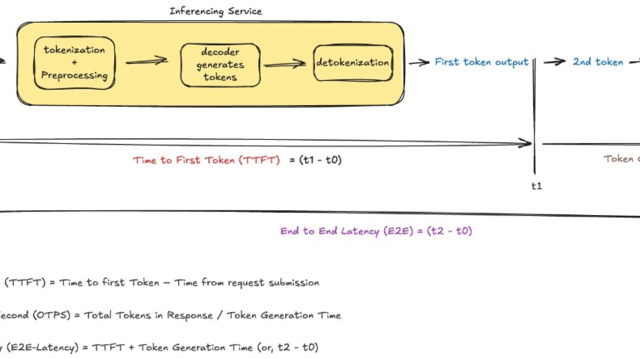
Latency in LLM applications is a multifaceted concept that goes beyond simple response times. When you interact with an LLM, you can receive responses in one of two ways: streaming or nonstreaming mode. In nonstreaming mode, you wait for the complete response before receiving any output—like waiting for someone to finish writing a letter. In streaming mode, you receive the response as it’s being generated—like watching someone type in real time.

To effectively optimize AI applications for responsiveness, we need to understand the key metrics that define latency and how they impact user experience. These metrics differ between streaming and nonstreaming modes and understanding them is crucial for building responsive AI applications.

Time to first token (TTFT) represents how quickly your streaming application starts responding. It’s the amount of time from when a user submits a request until they receive the beginning of a response (the first word, token, or chunk). Think of it as the initial reaction time of your AI application.

TTFT is affected by several factors:

• Length of your input prompt (longer prompts generally mean higher TTFT)
• Network conditions and geographic location (if the prompt is getting processed in a different region, it will take longer)

Calculation: TTFT = Time to first chunk/token – Time from request submission
Interpretation: Lower is better

Output tokens per second (OTPS) indicates how quickly your model generates new tokens after it starts responding. This metric is crucial for understanding the actual throughput of your model and how it maintains its response speed throughout longer generations.

OTPS is influenced by:

• Model size and complexity
• Length of the generated response
• Complexity of the task and prompt
• System load and resource availability

Calculation: OTPS = Total number of output tokens / Total generation time
Interpretation: Higher is better

End-to-end latency (E2E) measures the total time from request to complete response. As illustrated in the figure above, this encompasses the entire interaction.

Key factors affecting this metric include:

• Input prompt length
• Requested output length
• Model processing speed
• Network conditions
• Complexity of the task and prompt
• Postprocessing requirements (for example, using Amazon Bedrock Guardrails or other quality checks)

Calculation: E2E latency = Time at completion of request – Time from request submission
Interpretation: Lower is better

Although these metrics provide a solid foundation for understanding latency, there are additional factors and considerations that can impact the perceived performance of LLM applications. These metrics are shown in the following diagram.

The role of tokenization

An often-overlooked aspect of latency is how different models tokenize text differently. Each model’s tokenization strategy is defined by its provider during training and can’t be modified. For example, a prompt that generates 100 tokens in one model might generate 150 tokens in another. When comparing model performance, remember that these inherent tokenization differences can affect perceived response times, even when the models are equally efficient. Awareness of this variation can help you better interpret latency differences between models and make more informed decisions when selecting models for your applications.

Understanding user experience

The psychology of waiting in AI applications reveals interesting patterns about user expectations and satisfaction. Users tend to perceive response times differently based on the context and complexity of their requests. A slight delay in generating a complex analysis might be acceptable, and even a small lag in a conversational exchange can feel disruptive. This understanding helps us set appropriate optimization priorities for different types of applications.

Consistency over speed

Consistent response times, even if slightly slower, often lead to better user satisfaction than highly variable response times with occasional quick replies. This is crucial for streaming responses and implementing optimization strategies.

Keeping users engaged

When processing times are longer, simple indicators such as “Processing your request” or “loading animations” messages help keep users engaged, especially during the initial response time. In such scenarios, you want to optimize for TTFT.

Balancing speed, quality, and cost

Output quality often matters more than speed. Users prefer accurate responses over quick but less reliable ones. Consider benchmarking your user experience to find the best latency for your use case, considering that most humans can’t read faster than 225 words per minute and therefore extremely fast response can hinder user experience.

By understanding these nuances, you can make more informed decisions to optimize your AI applications for better user experience.

Latency-optimized inference: A deep dive

Amazon Bedrock latency-optimized inference capabilities are designed to provide higher OTPS and quicker TTFT, enabling applications to handle workloads more reliably. This optimization is available in the US East (Ohio) AWS Region for select FMs, including Anthropic’s Claude 3.5 Haiku and Meta’s Llama 3.1 models (both 405B and 70B versions). The optimization supports the following models:

• Higher OTPS – Faster token generation after the model starts responding
• Quicker TTFT – Faster initial response time

Implementation

To enable latency optimization, you need to set the latency parameter to optimized in your API calls:

# Using converse api without streaming
response = bedrock_runtime.converse(
    modelId='us.anthropic.claude-3-5-haiku-20241022-v1:0',
    messages=[{
            'role': 'user',
            'content': [{
                'text':'Write a story about music generating AI models'
                }]
              }],
    performanceConfig={'latency': 'optimized'}
)

For streaming responses:

# using converse API with streaming
response = bedrock_runtime.converse_stream(
       modelId='us.anthropic.claude-3-5-haiku-20241022-v1:0',
       messages=[{
            'role': 'user',
            'content': [{
                'text':'Write a story about music generating AI models'
                }]
              }],
        performanceConfig={'latency': 'optimized'}
    )

Benchmarking methodology and results

To understand the performance gains both for TTFT and OTPS, we conducted an offline experiment with around 1,600 API calls spread across various hours of the day and across multiple days. We used a dummy dataset comprising different task types: sequence-counting, story-writing, summarization, and translation. The input prompt ranged from 100 tokens to 100,000 tokens, and the output tokens ranged from 100 to 1,000 output tokens. These tasks were chosen to represent varying complexity levels and various model output lengths. Our test setup was hosted in the US West (Oregon) us-west-2 Region, and both the optimized and standard models were hosted in US East (Ohio) us-east-2 Region. This cross-Region setup introduced realistic network variability, helping us measure performance under conditions similar to real-world applications.

When analyzing the results, we focused on the key latency metrics discussed earlier: TTFT and OTPS. As a quick recap, lower TTFT values indicate faster initial response times, and higher OTPS values represent faster token generation speeds. We also looked at the 50th percentile (P50) and 90th percentile (P90) values to understand both typical performance and performance boundaries under challenging or upper bound conditions. Following the central limit theorem, we observed that, with sufficient samples, our results converged toward consistent values, providing reliable performance indicators.

It’s important to note that these results are from our specific test environment and datasets. Your actual results may vary based on your specific use case, prompt length, expected model response length, network conditions, client location, and other implementation components. When conducting your own benchmarks, make sure your test dataset represents your actual production workload characteristics, including typical input lengths and expected output patterns.

Benchmark results

Our experiments with the latency-optimized models revealed substantial performance improvements across both TTFT and OTPS metrics. The results in the following table show the comparison between standard and optimized versions of Anthropic’s Claude 3.5 Haiku and Meta’s Llama 3.1 70B models. For each model, we ran multiple iterations of our test scenarios to promote reliable performance. The improvements were particularly notable in high-percentile measurements, suggesting more consistent performance even under challenging conditions.

These results demonstrate significant improvements across all metrics for both models. For Anthropic’s Claude 3.5 Haiku model, the optimized version achieved up to 42.20% reduction in TTFT P50 and up to 51.70% reduction in TTFT P90, indicating more consistent initial response times. Additionally, the OTPS saw improvements of up to 77.34% at the P50 level and up to 125.50% at the P90 level, enabling faster token generation.

The gains for Meta’s Llama 3.1 70B model are even more impressive, with the optimized version achieving up to 51.65% reduction in TTFT P50 and up to 97.10% reduction in TTFT P90, providing consistently rapid initial responses. Furthermore, the OTPS saw a massive boost, with improvements of up to 353.84% at the P50 level and up to 529.33% at the P90 level, enabling up to 5x faster token generation in some scenarios.

Although these benchmark results show the powerful impact of latency-optimized inference, they represent just one piece of the optimization puzzle. To make best use of these performance improvements and achieve the best possible response times for your specific use case, you’ll need to consider additional optimization strategies beyond merely enabling the feature.

Comprehensive guide to LLM latency optimization

Even though Amazon Bedrock latency-optimized inference offers great improvements from the start, getting the best performance requires a well-rounded approach to designing and implementing your application. In the next section, we explore some other strategies and considerations to make your application as responsive as possible.

Prompt engineering for latency optimization

When optimizing LLM applications for latency, the way you craft your prompts affects both input processing and output generation.

To optimize your input prompts, follow these recommendations:

• Keep prompts concise – Long input prompts take more time to process and increase TTFT. Create short, focused prompts that prioritize necessary context and information.
• Break down complex tasks – Instead of handling large tasks in a single request, break them into smaller, manageable chunks. This approach helps maintain responsiveness regardless of task complexity.
• Smart context management – For interactive applications such as chatbots, include only relevant context instead of entire conversation history.
• Token management – Different models tokenize text differently, meaning the same input can result in different numbers of tokens. Monitor and optimize token usage to keep performance consistent. Use token budgeting to balance context preservation with performance needs.

To engineer for brief outputs, follow these recommendations:

• Engineer for brevity – Include explicit length constraints in your prompts (for example, “respond in 50 words or less”)
• Use system messages – Set response length constraints through system messages
• Balance quality and length – Make sure response constraints don’t compromise output quality

One of the best ways to make your AI application feel faster is to use streaming. Instead of waiting for the complete response, streaming shows the response as it’s being generated—like watching someone type in real-time. Streaming the response is one of the most effective ways to improve perceived performance in LLM applications maintaining user engagement.

These techniques can significantly reduce token usage and generation time, improving both latency and cost-efficiency.

Building production-ready AI applications

Although individual optimizations are important, production applications require a holistic approach to latency management. In this section, we explore how different system components and architectural decisions impact overall application responsiveness.

System architecture and end-to-end latency considerations

In production environments, overall system latency extends far beyond model inference time. Each component in your AI application stack contributes to the total latency experienced by users. For instance, when implementing responsible AI practices through Amazon Bedrock Guardrails, you might notice a small additional latency overhead. Similar considerations apply when integrating content filtering, user authentication, or input validation layers. Although each component serves a crucial purpose, their cumulative impact on latency requires careful consideration during system design.

Geographic distribution plays a significant role in application performance. Model invocation latency can vary considerably depending on whether calls originate from different Regions, local machines, or different cloud providers. This variation stems from data travel time across networks and geographic distances. When designing your application architecture, consider factors such as the physical distance between your application and model endpoints, cross-Region data transfer times, and network reliability in different Regions. Data residency requirements might also influence these architectural choices, potentially necessitating specific Regional deployments.

Integration patterns significantly impact how users perceive application performance. Synchronous processing, although simpler to implement, might not always provide the best user experience. Consider implementing asynchronous patterns where appropriate, such as pre-fetching likely responses based on user behavior patterns or processing noncritical components in the background. Request batching for bulk operations can also help optimize overall system throughput, though it requires careful balance with response time requirements.

As applications scale, additional infrastructure components become necessary but can impact latency. Load balancers, queue systems, cache layers, and monitoring systems all contribute to the overall latency budget. Understanding these components’ impact helps in making informed decisions about infrastructure design and optimization strategies.

Complex tasks often require orchestrating multiple model calls or breaking down problems into subtasks. Consider a content generation system that first uses a fast model to generate an outline, then processes different sections in parallel, and finally uses another model for coherence checking and refinement. This orchestration approach requires careful attention to cumulative latency impact while maintaining output quality. Each step needs appropriate timeouts and fallback mechanisms to provide reliable performance under various conditions.

Prompt caching for enhanced performance

Although our focus is on latency-optimized inference, it’s worth noting that Amazon Bedrock also offers prompt caching (in preview) to optimize for both cost and latency. This feature is particularly valuable for applications that frequently reuse context, such as document-based chat assistants or applications with repetitive query patterns. When combined with latency-optimized inference, prompt caching can provide additional performance benefits by reducing the processing overhead for frequently used contexts.

Prompt routing for intelligent model selection

Similar to prompt caching, Amazon Bedrock Intelligent Prompt Routing (in preview) is another powerful optimization feature. This capability automatically directs requests to different models within the same model family based on the complexity of each prompt. For example, simple queries can be routed to faster, more cost-effective models, and complex requests that require deeper understanding are directed to more sophisticated models. This automatic routing helps optimize both performance and cost without requiring manual intervention.

Architectural considerations and caching

Application architecture plays a crucial role in overall latency optimization. Consider implementing a multitiered caching strategy that includes response caching for frequently requested information and smart context management for historical information. This isn’t only about storing exact matches—consider implementing semantic caching that can identify and serve responses to similar queries.

Balancing model sophistication, latency, and cost

In AI applications, there’s a constant balancing act between model sophistication, latency, and cost, as illustrated in the diagram. Although more advanced models often provide higher quality outputs, they might not always meet strict latency requirements. In such cases, using a less sophisticated but faster model might be the better choice. For instance, in applications requiring near-instantaneous responses, opting for a smaller, more efficient model could be necessary to meet latency goals, even if it means a slight trade-off in output quality. This approach aligns with the broader need to optimize the interplay between cost, speed, and quality in AI systems.

Features such as Amazon Bedrock Intelligent Prompt Routing help manage this balance effectively. By automatically handling model selection based on request complexity, you can optimize for all three factors—quality, speed, and cost—without requiring developers to commit to a single model for all requests.

As we’ve explored throughout this post, optimizing LLM application latency involves multiple strategies, from using latency-optimized inference and prompt caching to implementing intelligent routing and careful prompt engineering. The key is to combine these approaches in a way that best suits your specific use case and requirements.

Conclusion

Making your AI application fast and responsive isn’t a one-time task, it’s an ongoing process of testing and improvement. Amazon Bedrock latency-optimized inference gives you a great starting point, and you’ll notice significant improvements when you combine it with the strategies we’ve discussed.

Ready to get started? Here’s what to do next:

1. Try our sample notebook to benchmark latency for your specific use case
2. Enable latency-optimized inference in your application code
3. Set up Amazon CloudWatch metrics to monitor your application’s performance

Remember, in today’s AI applications, being smart isn’t enough, being responsive is just as important. Start implementing these optimization strategies today and watch your application’s performance improve.

About the Authors

Ishan Singh is a Generative AI Data Scientist at Amazon Web Services, where he helps customers build innovative and responsible generative AI solutions and products. With a strong background in AI/ML, Ishan specializes in building Generative AI solutions that drive business value. Outside of work, he enjoys playing volleyball, exploring local bike trails, and spending time with his wife and dog, Beau.

Yanyan Zhang is a Senior Generative AI Data Scientist at Amazon Web Services, where she has been working on cutting-edge AI/ML technologies as a Generative AI Specialist, helping customers use generative AI to achieve their desired outcomes. Yanyan graduated from Texas A&M University with a PhD in Electrical Engineering. Outside of work, she loves traveling, working out, and exploring new things.

Rupinder Grewal is a Senior AI/ML Specialist Solutions Architect with AWS. He currently focuses on serving of models and MLOps on Amazon SageMaker. Prior to this role, he worked as a Machine Learning Engineer building and hosting models. Outside of work, he enjoys playing tennis and biking on mountain trails.

Vivek Singh is a Senior Manager, Product Management at AWS AI Language Services team. He leads the Amazon Transcribe product team. Prior to joining AWS, he held product management roles across various other Amazon organizations such as consumer payments and retail. Vivek lives in Seattle, WA and enjoys running, and hiking.

Ankur Desai is a Principal Product Manager within the AWS AI Services team.

Read More

Evaluating large language models (LLMs) is crucial as LLM-based systems become increasingly powerful and relevant in our society. Rigorous testing allows us to understand an LLM’s capabilities, limitations, and potential biases, and provide actionable feedback to identify and mitigate risk. Furthermore, evaluation processes are important not only for LLMs, but are becoming essential for assessing prompt template quality, input data quality, and ultimately, the entire application stack. As LLMs take on more significant roles in areas like healthcare, education, and decision support, robust evaluation frameworks are vital for building trust and realizing the technology’s potential while mitigating risks.

Developers interested in using LLMs should prioritize a comprehensive evaluation process for several reasons. First, it assesses the model’s suitability for specific use cases, because performance can vary significantly across different tasks and domains. Evaluations are also a fundamental tool during application development to validate the quality of prompt templates. This process makes sure that solutions align with the company’s quality standards and policy guidelines before deploying them to production. Regular interval evaluation also allows organizations to stay informed about the latest advancements, making informed decisions about upgrading or switching models. Moreover, a thorough evaluation framework helps companies address potential risks when using LLMs, such as data privacy concerns, regulatory compliance issues, and reputational risk from inappropriate outputs. By investing in robust evaluation practices, companies can maximize the benefits of LLMs while maintaining responsible AI implementation and minimizing potential drawbacks.

To support robust generative AI application development, it’s essential to keep track of models, prompt templates, and datasets used throughout the process. This record-keeping allows developers and researchers to maintain consistency, reproduce results, and iterate on their work effectively. By documenting the specific model versions, fine-tuning parameters, and prompt engineering techniques employed, teams can better understand the factors contributing to their AI system’s performance. Similarly, maintaining detailed information about the datasets used for training and evaluation helps identify potential biases and limitations in the model’s knowledge base. This comprehensive approach to tracking key components not only facilitates collaboration among team members but also enables more accurate comparisons between different iterations of the AI application. Ultimately, this systematic approach to managing models, prompts, and datasets contributes to the development of more reliable and transparent generative AI applications.

In this post, we show how to use FMEval and Amazon SageMaker to programmatically evaluate LLMs. FMEval is an open source LLM evaluation library, designed to provide data scientists and machine learning (ML) engineers with a code-first experience to evaluate LLMs for various aspects, including accuracy, toxicity, fairness, robustness, and efficiency. In this post, we only focus on the quality and responsible aspects of model evaluation, but the same approach can be extended by using other libraries for evaluating performance and cost, such as LLMeter and FMBench, or richer quality evaluation capabilities like those provided by Amazon Bedrock Evaluations.

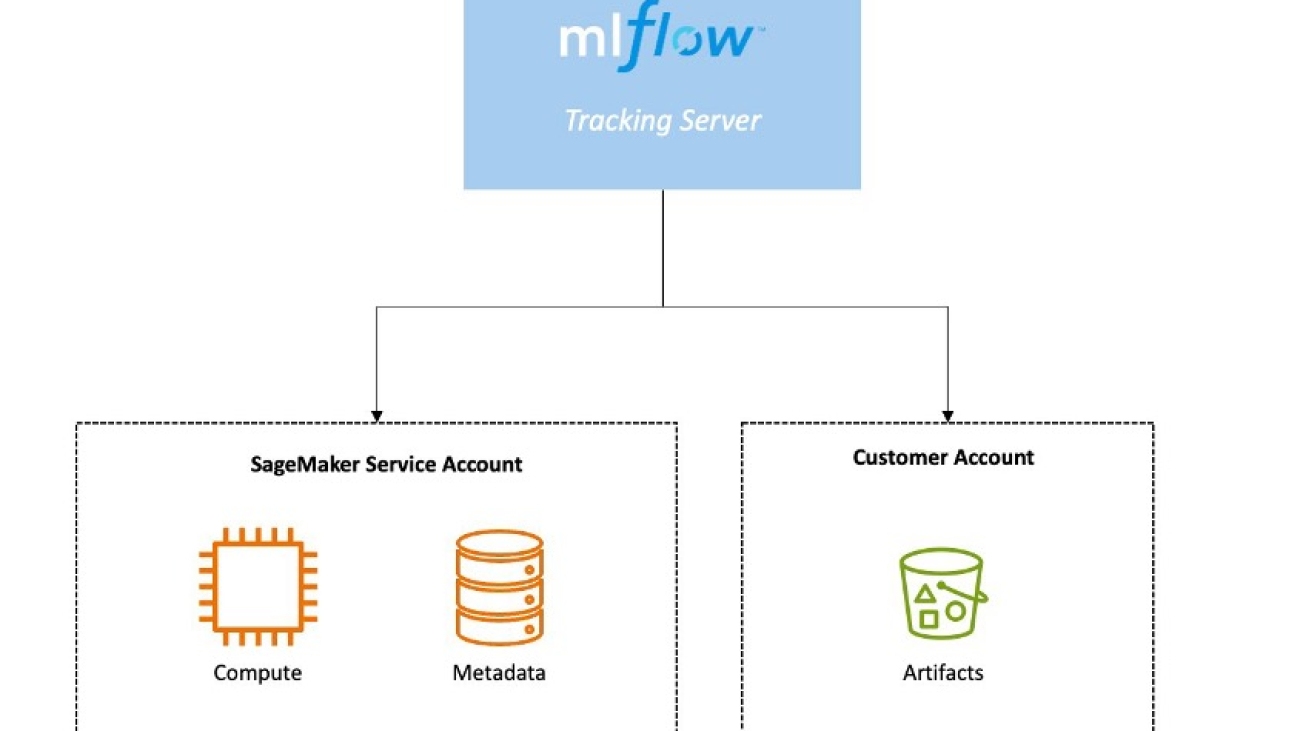
SageMaker is a data, analytics, and AI/ML platform, which we will use in conjunction with FMEval to streamline the evaluation process. We specifically focus on SageMaker with MLflow. MLflow is an open source platform for managing the end-to-end ML lifecycle, including experimentation, reproducibility, and deployment. The managed MLflow in SageMaker simplifies the deployment and operation of tracking servers, and offers seamless integration with other AWS services, making it straightforward to track experiments, package code into reproducible runs, and share and deploy models.

By combining FMEval’s evaluation capabilities with SageMaker with MLflow, you can create a robust, scalable, and reproducible workflow for assessing LLM performance. This approach can enable you to systematically evaluate models, track results, and make data-driven decisions in your generative AI development process.

Using FMEval for model evaluation

FMEval is an open-source library for evaluating foundation models (FMs). It consists of three main components:

• Data config – Specifies the dataset location and its structure.
• Model runner – Composes input, and invokes and extracts output from your model. Thanks to this construct, you can evaluate any LLM by configuring the model runner according to your model.
• Evaluation algorithm – Computes evaluation metrics to model outputs. Different algorithms have different metrics to be specified.

You can use pre-built components because it provides native components for both Amazon Bedrock and Amazon SageMaker JumpStart, or create custom ones by inheriting from the base core component. The library supports various evaluation scenarios, including pre-computed model outputs and on-the-fly inference. FMEval offers flexibility in dataset handling, model integration, and algorithm implementation. Refer to Evaluate large language models for quality and responsibility or the Evaluating Large Language Models with fmeval paper to dive deeper into FMEval, or see the official GitHub repository.

Using SageMaker with MLflow to track experiments

The fully managed MLflow capability on SageMaker is built around three core components:

• MLflow tracking server – This component can be quickly set up through the Amazon SageMaker Studio interface or using the API for more granular configurations. It functions as a standalone HTTP server that provides various REST API endpoints for monitoring, recording, and visualizing experiment runs. This allows you to keep track of your ML experiments.
• MLflow metadata backend – This crucial part of the tracking server is responsible for storing all the essential information about your experiments. It keeps records of experiment names, run identifiers, parameter settings, performance metrics, tags, and locations of artifacts. This comprehensive data storage makes sure that you can effectively manage and analyze your ML projects.
• MLflow artifact repository – This component serves as a storage space for all the files and objects generated during your ML experiments. These can include trained models, datasets, log files, and visualizations. The repository uses an Amazon Simple Storage Service (Amazon S3) bucket within your AWS account, making sure that your artifacts are stored securely and remain under your control.

The following diagram depicts the different components and where they run within AWS.

Code walkthrough

You can follow the full sample code from the GitHub repository.

Prerequisites

You must have the following prerequisites:

• A running MLflow tracking server within an Amazon SageMaker Studio domain
• A JupyterLab application within the same SageMaker Studio domain
• Active subscriptions to the Amazon Bedrock models you want to evaluate and permissions to invoke these models
• Permissions to deploy foundation models via Amazon SageMaker JumpStart

Refer to the documentation best practices regarding AWS Identity and Access Management (IAM) policies for SageMaker, MLflow, and Amazon Bedrock on how to set up permissions for the SageMaker execution role. Remember to always following the least privilege access principle.

Evaluate a model and log to MLflow

We provide two sample notebooks to evaluate models hosted in Amazon Bedrock (Bedrock.ipynb) and models deployed to SageMaker Hosting using SageMaker JumpStart (JumpStart.ipynb). The workflow implemented in these two notebooks is essentially the same, although a few differences are noteworthy:

• Models hosted in Amazon Bedrock can be consumed directly using an API without any setup, providing a “serverless” experience, whereas models in SageMaker JumpStart require the user first to deploy the models. Although deploying models through SageMaker JumpStart is a straightforward operation, the user is responsible for managing the lifecycle of the endpoint.
• ModelRunners implementations differ. FMEval provides native implementations for both Amazon Bedrock, using the BedrockModelRunner class, and SageMaker JumpStart, using the JumpStartModelRunner class. We discuss the main differences in the following section.

ModelRunner definition

For BedrockModelRunner, we need to find the model content_template. We can find this information conveniently on the Amazon Bedrock console in the API request sample section, and look at value of the body. The following example is the content template for Anthropic’s Claude 3 Haiku:

output_jmespath = "content[0].text"
content_template = """{
  "anthropic_version": "bedrock-2023-05-31",
  "max_tokens": 512,
  "temperature": 0.5,
  "messages": [
    {
      "role": "user",
      "content": [
        {
          "type": "text",
          "text": $prompt
        }
      ]
    }
  ]
}"""

model_runner = BedrockModelRunner(
    model_id=model_id,
    output=output_jmespath,
    content_template=content_template,
)

For JumpStartModelRunner, we need to find the model and model_version. This information can be retrieved directly using the get_model_info_from_endpoint(endpoint_name=endpoint_name) utility provided by the SageMaker Python SDK, where endpoint_name is the name of the SageMaker endpoint where the SageMaker JumpStart model is hosted. See the following code example:

from sagemaker.jumpstart.session_utils import get_model_info_from_endpoint

model_id, model_version, , , _ = get_model_info_from_endpoint(endpoint_name=endpoint_name)

model_runner = JumpStartModelRunner(
    endpoint_name=endpoint_name,
    model_id=model_id,
    model_version=model_version,
)

DataConfig definition

For each model runner, we want to evaluate three categories: Summarization, Factual Knowledge, and Toxicity. For each of this category, we prepare a DataConfig object for the appropriate dataset. The following example shows only the data for the Summarization category:

dataset_path = Path("datasets")

dataset_uri_summarization = dataset_path / "gigaword_sample.jsonl"
if not dataset_uri_summarization.is_file():
    print("ERROR - please make sure the file, gigaword_sample.jsonl, exists.")

data_config_summarization = DataConfig(
    dataset_name="gigaword_sample",
    dataset_uri=dataset_uri_summarization.as_posix(),
    dataset_mime_type=MIME_TYPE_JSONLINES,
    model_input_location="document",
    target_output_location="summary",
)

Evaluation sets definition

We can now create an evaluation set for each algorithm we want to use in our test. For the Summarization evaluation set, replace with your own prompt according to the input signature identified earlier. fmeval uses $model_input as placeholder to get the input from your evaluation dataset. See the following code:

summarization_prompt = "Summarize the following text in one sentence: $model_input"

summarization_accuracy = SummarizationAccuracy()

evaluation_set_summarization = EvaluationSet(
  data_config_summarization,
  summarization_accuracy,
  summarization_prompt,
)

We are ready now to group the evaluation sets:

evaluation_list = [
    evaluation_set_summarization,
    evaluation_set_factual,
    evaluation_set_toxicity,
]

Evaluate and log to MLflow

We set up the MLflow experiment used to track the evaluations. We then create a new run for each model, and run all the evaluations for that model within that run, so that the metrics will all appear together. We use the model_id as the run name to make it straightforward to identify this run as part of a larger experiment, and run the evaluation using the run_evaluation_sets() defined in utils.py. See the following code:

run_name = f"{model_id}"

experiment_name = "fmeval-mlflow-simple-runs"
experiment = mlflow.set_experiment(experiment_name)

with mlflow.start_run(run_name=run_name) as run:
    run_evaluation_sets(model_runner, evaluation_list)

It is up to the user to decide how to best organize the results in MLflow. In fact, a second possible approach is to use nested runs. The sample notebooks implement both approaches to help you decide which one fits best your needs.

experiment_name = "fmeval-mlflow-nested-runs"
experiment = mlflow.set_experiment(experiment_name)

with mlflow.start_run(run_name=run_name, nested=True) as run:
    run_evaluation_sets_nested(model_runner, evaluation_list)

Run evaluations

Tracking the evaluation process involves storing information about three aspects:

• The input dataset
• The parameters of the model being evaluated
• The scores for each evaluation

We provide a helper library (fmeval_mlflow) to abstract the logging of these aspects to MLflow, streamlining the interaction with the tracking server. For the information we want to store, we can refer to the following three functions:

• log_input_dataset(data_config: DataConfig | list[DataConfig]) – Log one or more input datasets to MLflow for evaluation purposes
• log_runner_parameters(model_runner: ModelRunner, custom_parameters_map: dict | None = None, model_id: str | None = None,) – Log the parameters associated with a given ModelRunner instance to MLflow
• log_metrics(eval_output: list[EvalOutput], log_eval_output_artifact: bool = False) – Log metrics and artifacts for a list of SingleEvalOutput instances to MLflow.

When the evaluations are complete, we can analyze the results directly in the MLflow UI for a first visual assessment.

In the following screenshots, we show the visualization differences between logging using simple runs or nested runs.

You might want to create your own custom visualizations. For example, spider plots are often used to make visual comparison across multiple metrics. In the notebook compare_models.ipynb, we provide an example on how to use metrics stored in MLflow to generate such plots, which ultimately can also be stored in MLflow as part of your experiments. The following screenshots show some example visualizations.

Clean up

Once created, an MLflow tracking server will incur costs until you delete or stop it. Billing for tracking servers is based on the duration the servers have been running, the size selected, and the amount of data logged to the tracking servers. You can stop the tracking servers when they are not in use to save costs or delete them using the API or SageMaker Studio UI. For more details on pricing, see Amazon SageMaker pricing.

Similarly, if you deployed a model using SageMaker, endpoints are priced by deployed infrastructure time rather than by requests. You can avoid unnecessary charges by deleting your endpoints when you’re done with the evaluation.

Conclusion

In this post, we demonstrated how to create an evaluation framework for LLMs by combining SageMaker managed MLflow with FMEval. This integration provides a comprehensive solution for tracking and evaluating LLM performance across different aspects including accuracy, toxicity, and factual knowledge.

To enhance your evaluation journey, you can explore the following:

• Get started with FMeval and SageMaker managed MLflow by following our code examples in the provided GitHub repository
• Implement systematic evaluation practices in your LLM development workflow using the demonstrated approach
• Use MLflow’s tracking capabilities to maintain detailed records of your evaluations, making your LLM development process more transparent and reproducible
• Explore different evaluation metrics and datasets available in FMEval to comprehensively assess your LLM applications

By adopting these practices, you can build more reliable and trustworthy LLM applications while maintaining a clear record of your evaluation process and results.

About the authors

Paolo Di Francesco is a Senior Solutions Architect at Amazon Web Services (AWS). He holds a PhD in Telecommunications Engineering and has experience in software engineering. He is passionate about machine learning and is currently focusing on using his experience to help customers reach their goals on AWS, in particular in discussions around MLOps. Outside of work, he enjoys playing football and reading.

Dr. Alessandro Cerè is a GenAI Evaluation Specialist and Solutions Architect at AWS. He assists customers across industries and regions in operationalizing and governing their generative AI systems at scale, ensuring they meet the highest standards of performance, safety, and ethical considerations. Bringing a unique perspective to the field of AI, Alessandro has a background in quantum physics and research experience in quantum communications and quantum memories. In his spare time, he pursues his passion for landscape and underwater photography.

Read More

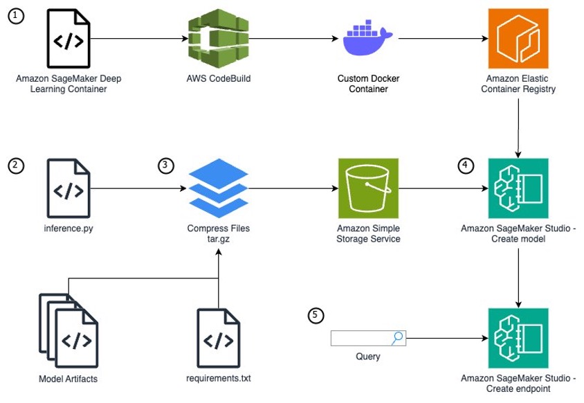
Amazon SageMaker provides a seamless experience for building, training, and deploying machine learning (ML) models at scale. Although SageMaker offers a wide range of built-in algorithms and pre-trained models through Amazon SageMaker JumpStart, there are scenarios where you might need to bring your own custom model or use specific software dependencies not available in SageMaker managed container images. Examples for this could include use cases like geospatial analysis, bioinformatics research, or quantum machine learning. In such cases, SageMaker allows you to extend its functionality by creating custom container images and defining custom model definitions. This approach enables you to package your model artifacts, dependencies, and inference code into a container image, which you can deploy as a SageMaker endpoint for real-time inference. This post walks you through the end-to-end process of deploying a single custom model on SageMaker using NASA’s Prithvi model. The Prithvi model is a first-of-its-kind temporal Vision transformer pre-trained by the IBM and NASA team on contiguous US Harmonised Landsat Sentinel 2 (HLS) data. It can be finetuned for image segmentation using the mmsegmentation library for use cases like burn scars detection, flood mapping, and multi-temporal crop classification. Due to its unique architecture and fine-tuning dependency on the MMCV library, it is an effective example of how to deploy complex custom models to SageMaker. We demonstrate how to use the flexibility of SageMaker to deploy your own custom model, tailored to your specific use case and requirements. Whether you’re working with unique model architectures, specialized libraries, or specific software versions, this approach empowers you to harness the scalability and management capabilities of SageMaker while maintaining control over your model’s environment and dependencies.

Solution overview

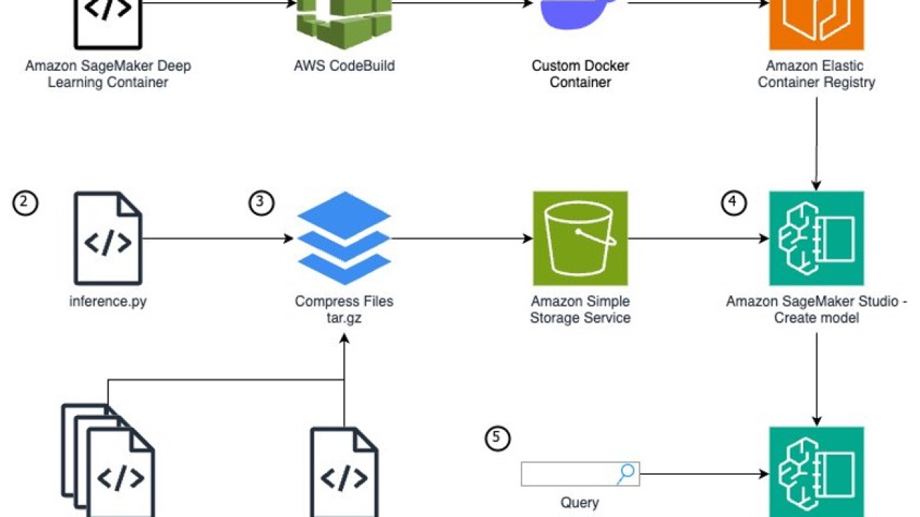
To run a custom model that needs unique packages as a SageMaker endpoint, you need to follow these steps:

1. If your model requires additional packages or package versions unavailable from the SageMaker managed container images, you will need to extend one of the container images. By extending a SageMaker managed container vs. creating one from scratch, you can focus on your specific use case and model development instead of the container infrastructure.
2. Write a Python model definition using the SageMaker inference.py file format.
3. Define your model artifacts and inference file within a specific file structure, archive your model files as a tar.gz file, and upload your files to Amazon Simple Storage Service (Amazon S3).
4. With your model code and an extended SageMaker container, use Amazon SageMaker Studio to create a model, endpoint configuration, and endpoint.
5. Query the inference endpoint to confirm your model is running correctly.

The following diagram illustrates the solution architecture and workflow:

Prerequisites

You need the following prerequisites before you can proceed. For this post, we use the us-east-1 AWS Region:

1. Have access to a POSIX based (Mac/Linux) system or SageMaker notebooks. This post doesn’t cover setting up SageMaker access and assumes a notebook accessible to the internet. However, this is not a security best practice and should not be done in production. To learn how to create a SageMaker notebook within a virtual private cloud (VPC), see Connect to SageMaker AI Within your VPC.
2. Make sure you have AWS Identity and Access Management (IAM) permissions for SageMaker access; S3 bucket create, read, and PutObject access; AWS CodeBuild access; Amazon Elastic Container Registry (Amazon ECR) repository access; and the ability to create IAM roles.
3. Download the Prithvi model artifacts and flood data fine-tuning:

   curl -s https://packagecloud.io/install/repositories/github/git-lfs/script.deb.sh | sudo bash 
   sudo apt-get install git-lfs 
   git lfs install 
   git clone https://huggingface.co/ibm-nasa-geospatial/Prithvi-100M 
   git clone https://huggingface.co/ibm-nasa-geospatial/Prithvi-100M-sen1floods11

Extend a SageMaker container image for your model

Although AWS provides pre-built container images optimized for deep learning on the AWS Deep Learning Containers (DLCs) GitHub for PyTorch and TensorFlow use cases, there are scenarios where models require additional libraries not included in these containers. The installation of these dependencies can take minutes or hours, so it’s more efficient to pre-build these dependencies into a custom container image. For this example, we deploy the Prithvi model, which is dependent on the MMCV library for advanced computer vision techniques. This library is not available within any of the SageMaker DLCs, so you will have to create an extended container to add it. Both MMCV and Prithvi are third-party models which have not undergone AWS security reviews, so please review these models yourself or use at your own risk. This post uses CodeBuild and a Docker Dockerfile to build the extended container.

Complete the following steps:

1. CodeBuild requires a source location containing the source code. Create an S3 bucket to serve as this source location using the following commands:

   # generate a unique postfix 
   BUCKET_POSTFIX=$(python3 -S -c "import uuid; print(str(uuid.uuid4().hex)[:10])") 
   echo "export BUCKET_POSTFIX=${BUCKET_POSTFIX}" >> ~/.bashrc 
   echo "Your bucket name will be customsagemakercontainer-codebuildsource-${BUCKET_POSTFIX}" 
   # make your bucket 
   aws s3 mb s3://customsagemakercontainer-codebuildsource-${BUCKET_POSTFIX}

2. Create an ECR repository to store the custom container image produced by the CodeBuild project. Record the repository URI as an environment variable.

   CONTAINER_REPOSITORY_NAME="prithvi" 
   aws ecr create-repository --repository-name ${CONTAINER_REPOSITORY_NAME} 
   export REPOSITORY_URI=$(aws ecr describe-repositories --repository-names ${CONTAINER_REPOSITORY_NAME} --query 'repositories[0].repositoryUri' --output text)

3. Create a Dockerfile for the custom container. You use an AWS Deep Learning SageMaker framework container as the base image because it includes required dependencies such as SageMaker libraries, PyTorch, and CUDA.

This Docker container installs the Prithvi model and MMCV v1.6.2. These models are third-party models not produced by AWS and therefore may have security vulnerabilities. Use at your own risk.

cat > Dockerfile << EOF 
FROM 763104351884.dkr.ecr.us-east-1.amazonaws.com/pytorch-inference:1.13.1-gpu-py39-cu117-ubuntu20.04-sagemaker
WORKDIR /root
RUN DEBIAN_FRONTEND=noninteractive apt-get update -y
RUN DEBIAN_FRONTEND=noninteractive apt-get upgrade -y
RUN git clone https://github.com/NASA-IMPACT/hls-foundation-os.git
RUN wget https://github.com/open-mmlab/mmcv/archive/refs/tags/v1.6.2.tar.gz
RUN tar xvzf v1.6.2.tar.gz
WORKDIR /root/hls-foundation-os
RUN pip install -e . 
RUN pip install -U openmim 
WORKDIR /root/mmcv-1.6.2
RUN MMCV_WITH_OPS=1 pip install -e . -v

EOF

4. Create a buildspec file to define the build process for the CodeBuild project. This buildspec file will instruct CodeBuild to install the nvidia-container-toolkit to make sure the Docker container has GPU access, run the Dockerfile build, and push the built container image to your ECR repository.

   cat > buildspec.yml << EOF
   version: 0.2
   
   phases:
       pre_build:
           commands:
           - echo Logging in to Amazon ECR...
           - IMAGE_TAG=sagemaker-gpu
           - curl -s -L https://nvidia.github.io/libnvidia-container/stable/rpm/nvidia-container-toolkit.repo | sudo tee /etc/yum.repos.d/nvidia-container-toolkit.repo
           - sudo yum install -y nvidia-container-toolkit
           - sudo nvidia-ctk runtime configure --runtime=docker
           - | 
             cat > /etc/docker/daemon.json << EOF
             {
                 "runtimes": {
                     "nvidia": {
                         "args": [],
                         "path": "nvidia-container-runtime"
                     }
                 },
                 "default-runtime": "nvidia"
             }
             EOF
           - kill $(ps aux | grep -v grep | grep "/usr/local/bin/dockerd --host" | awk '{print $2}')
           - sleep 10
           - nohup /usr/local/bin/dockerd --host=unix:///var/run/docker.sock --host=tcp://127.0.0.1:2375 --storage-driver=overlay2 &
           - sleep 10
           - aws ecr get-login-password --region $AWS_REGION | docker login --username AWS --password-stdin $REPOSITORY_URI_AWSDL
           - docker pull $REPOSITORY_URI_AWSDL/pytorch-inference:1.13.1-gpu-py39-cu117-ubuntu20.04-sagemaker
   
       build:
           commands:
           - echo Build started at $(date)
           - echo Building the Docker image...
           - aws ecr get-login-password --region $AWS_REGION | docker login --username AWS --password-stdin $REPOSITORY_URI
           - DOCKER_BUILDKIT=0 docker build -t $REPOSITORY_URI:latest .
           - docker tag $REPOSITORY_URI:latest $REPOSITORY_URI:$IMAGE_TAG
   
       post_build:
           commands:
           - echo Build completed at $(date)
           - echo Pushing the Docker images...
           - docker push $REPOSITORY_URI:latest
           - docker push $REPOSITORY_URI:$IMAGE_TAG
   
   EOF

5. Zip and upload the Dockerfile and buildspec.yml files to the S3 bucket. This zip file will serve as the source code for the CodeBuild project.
   • To install zip on a SageMaker notebook, run the following command:

     sudo apt install zip

   • With zip installed, run the following command:

     zip prithvi_container_source.zip Dockerfile buildspec.yml
     aws s3 cp prithvi_container_source.zip s3://customsagemakercontainer-codebuildsource-${BUCKET_POSTFIX}/

6. Create a CodeBuild service role so CodeBuild can access the required AWS services for the build.
   • First, create a file defining the role’s trust policy:

     cat > create-role.json << EOF
     {
       "Version": "2012-10-17",
       "Statement": [
         {
           "Effect": "Allow",
           "Principal": {
             "Service": "codebuild.amazonaws.com"
           },
           "Action": "sts:AssumeRole"
         }
       ]
     }
     EOF

   • Create a file defining the service role’s permissions. This role has a few wildcard permissions (/* or *). These can give more permissions than needed and break the rule of least privilege. For more information about defining least privilege for production use cases, see Grant least privilege.

     cat > put-role-policy.json << EOF
     {
       "Version": "2012-10-17",
       "Statement": [
         {
           "Sid": "CloudWatchLogsPolicy",
           "Effect": "Allow",
           "Action": [
             "logs:CreateLogGroup",
             "logs:CreateLogStream",
             "logs:PutLogEvents"
           ],
           "Resource": "arn:aws:logs:us-east-1:*:log-group:/aws/codebuild/*:*"
         },
         {
           "Sid": "S3GetObjectPolicy",
           "Effect": "Allow",
           "Action": [
             "s3:GetObject",
             "s3:GetObjectVersion"
           ],
           "Resource": [
             "arn:aws:s3:::customsagemakercontainer-codebuildsource-${BUCKET_POSTFIX}",
             "arn:aws:s3:::customsagemakercontainer-codebuildsource-${BUCKET_POSTFIX}/*"
             ]
         },
         {
           "Sid": "S3BucketIdentity",
           "Effect": "Allow",
           "Action": [
             "s3:GetBucketAcl",
             "s3:GetBucketLocation"
           ],
           "Resource": "arn:aws:s3:::customsagemakercontainer-codebuildsource-${BUCKET_POSTFIX}"
         },
         {
           "Sid": "ECRAccess",
           "Effect": "Allow",
           "Action": [
             "ecr:GetImage",
             "ecr:BatchGetImage",
             "ecr:BatchCheckLayerAvailability",
             "ecr:CompleteLayerUpload",
             "ecr:UploadLayerPart",
             "ecr:GetDownloadUrlForLayer",
             "ecr:InitiateLayerUpload",
             "ecr:PutImage",
             "ecr:ListImages",
             "ecr:DescribeRepositories",
             "ecr:DescribeImages",
             "ecr:DescribeRegistry",
             "ecr:TagResource"
           ],
           "Resource": ["arn:aws:ecr:*:*:repository/prithvi",
                         "arn:aws:ecr:*:763104351884:repository/*"]
         },
         {
           "Sid": "ECRAuthToken",
           "Effect": "Allow",
           "Action": [
             "ecr:GetAuthorizationToken"
           ],
           "Resource": "*"
         }
       ]
     }
     EOF

   • Create the CodeBuild service role:

     aws iam create-role --role-name CodeBuildServiceRole --assume-role-policy-document file://create-role.json

7. Capture the name of the role Amazon Resource Name (ARN) from the CLI command response and record as an environment variable:

   export CODEBUILD_SERVICE_ROLE_ARN=$(aws iam get-role --role-name CodeBuildServiceRole --query 'Role.Arn' --output text)

8. Attach the permission policies to the service role:

   aws iam put-role-policy --role-name CodeBuildServiceRole --policy-name CodeBuildServiceRolePolicy --policy-document file://put-role-policy.json

9. Define the configurations for the CodeBuild build project using the build project JSON specification:

   cat > codebuild-project.json << EOF
   {
       "name": "prithvi-container-build",
       "description": "build process to modify the AWS SageMaker Deep Learning Container to include HLS/Prithvi",
       "source": {
         "type": "S3",
         "location": "customsagemakercontainer-codebuildsource-${BUCKET_POSTFIX}/prithvi_container_source.zip",
         "buildspec": "buildspec.yml",
         "insecureSsl": false
       },
       "artifacts": {
         "type": "NO_ARTIFACTS"
       },
       "cache": {
         "type": "NO_CACHE"
       },
       "environment": {
         "type": "LINUX_GPU_CONTAINER",
         "image": "aws/codebuild/amazonlinux2-x86_64-standard:5.0",
         "computeType": "BUILD_GENERAL1_SMALL",
         "environmentVariables": [
           {
             "name": "REPOSITORY_URI_AWSDL",
             "value": "763104351884.dkr.ecr.us-east-1.amazonaws.com",
             "type": "PLAINTEXT"
           },
           {
             "name": "AWS_REGION",
             "value": "us-east-1",
             "type": "PLAINTEXT"
           },
           {
               "name": "REPOSITORY_URI",
               "value": "$REPOSITORY_URI",
               "type": "PLAINTEXT"
             }
         ],
         "imagePullCredentialsType": "CODEBUILD",
         "privilegedMode": true
       },
       "serviceRole": "$CODEBUILD_SERVICE_ROLE_ARN",
       "timeoutInMinutes": 60,
       "queuedTimeoutInMinutes": 480,
       "logsConfig": {
         "cloudWatchLogs": {
           "status": "ENABLED"
         }
     }
   }
   EOF

10. Create the CodeBuild project using the codebuild-project.json specification defined in the previous step:

    aws codebuild create-project --cli-input-json file://codebuild-project.json

11. Run a build for the CodeBuild project:

    aws codebuild start-build --project-name prithvi-container-build

The build will take approximately 30 minutes to complete and cost approximately $1.50 to run. The CodeBuild compute instance type gpu1.small costs $0.05 per minute.

After you run the preceding command, you can press Ctrl+C to exit and run future commands. The build will already be running on AWS and will not be canceled by closing the command.

12. Monitor the status of the build using the following command and wait until you observe buildStatus=SUCCEEDED before proceeding to the next step:

    export BUILD_ID=$(aws codebuild list-builds-for-project --project-name prithvi-container-build --query 'ids[0]' --output text) aws codebuild batch-get-builds --ids ${BUILD_ID} | grep buildStatus

After your CodeBuild project has completed, make sure that you do not close your terminal. The environment variables here will be used again.

Build your inference.py file

To run a custom model for inference on AWS, you need to build out an inference.py file that initializes your model, defines the input and output structure, and produces your inference results. In this file, you must define four functions:

• model_fn – Initializes your model
•  input_fn – Defines how your data should be input and how to convert to a usable format
• predict_fn – Takes the input data and receives the prediction
• output_fn – Converts the prediction into an API call format

We use the following completed inference.py file for the SageMaker endpoint in this post. Download this inference.py to continue because it includes the helper functions to process the TIFF files needed for this model’s input. The following code is contained within the inference.py and is only shown to provide an explanation of what is being done in the file.

model_fn

The model_fn function builds your model, which is called and used within the predict_fn function. This function loads the model weights into a torch model checkpoint, opens the model config, defines global variables, instantiates the model, loads the model checkpoint into the model, and returns the model.

def model_fn(model_dir):
    # implement custom code to load the model
    # load weights
    weights_path = "./code/prithvi/Prithvi_100M.pt"
    checkpoint = torch.load(weights_path, map_location="cpu")

    # read model config
    model_cfg_path = "./code/prithvi/Prithvi_100M_config.yaml"
    with open(model_cfg_path) as f:
        model_config = yaml.safe_load(f)

    model_args, train_args = model_config["model_args"], model_config["train_params"]

    global means
    global stds
    means = np.array(train_args["data_mean"]).reshape(-1, 1, 1)
    stds = np.array(train_args["data_std"]).reshape(-1, 1, 1)
    # let us use only 1 frame for now (the model was trained on 3 frames)
    model_args["num_frames"] = 1

    # instantiate model
    model = MaskedAutoencoderViT(**model_args)
    model.eval()

    # load weights into model
    # strict=false because we are loading with only 1 frame, but the warning is expected
    del checkpoint['pos_embed']
    del checkpoint['decoder_pos_embed']
    _ = model.load_state_dict(checkpoint, strict=False)
    
    return model

input_fn

This function defines the expected input for the model and how to load the input for use in predict_fn. The endpoint expects a string URL path linked to a TIFF file you can find online from the Prithvi demo on Hugging Face. This function also defines the content type of the request sent in the body (such as application/json, image/tiff).

def input_fn(input_data, content_type):
    # decode the input data  (e.g. JSON string -> dict)
    # statistics used to normalize images before passing to the model
    raster_data = load_raster(input_data, crop=(224, 224))
    return raster_data

predict_fn:

In predict_fn, you create the prediction from the given input. In this case, creating the prediction image uses two helper functions specific to this endpoint (preprocess_image and enhance_raster_for_visualization). You can find both functions here. The preprocess_image function normalizes the image, then the function uses torch.no_grad to disable gradient calculations for the model. This is useful during inference to decrease inference time and reduce memory usage. Next, the function collects the prediction from the instantiated model. The mask ratio determines the number of pixels on the image zeroed out during inference. The two unpatchify functions convert the smaller patchified results produced by the model back to the original image space. The function normalized.clone() clones the normalized images and replaces the masked Regions from rec_img with the Regions from the pred_img. Finally, the function reshapes the image back into TIFF format, removes the normalization, and returns the image in raster format, which is valuable for visualization. The result of this is an image that can be converted to bytes for the user and then visualized on the user’s screen.

def predict_fn(data, model):
    normalized = preprocess_image(data)
    with torch.no_grad():
        mask_ratio = 0.5
        _, pred, mask = model(normalized, mask_ratio=mask_ratio)
        mask_img = model.unpatchify(mask.unsqueeze(-1).repeat(1, 1, pred.shape[-1])).detach().cpu()
        pred_img = model.unpatchify(pred).detach().cpu()#.numpy()
        rec_img = normalized.clone()
        rec_img[mask_img == 1] = pred_img[mask_img == 1]
        rec_img_np = (rec_img.numpy().reshape(6, 224, 224) * stds) + means
        print(rec_img_np.shape)
        return enhance_raster_for_visualization(rec_img_np, ref_img=data)

output_fn

output_fn returns the TIFF image received from predict_fn as an array of bytes.

def output_fn(prediction, accept):
    print(prediction.shape)
    return prediction.tobytes()

Test your inference.py file

Now that you have downloaded the complete inference.py file, there are two options to test your model before compressing the files and uploading them to Amazon S3:

• Test the inference.py functions on your custom container within an Amazon Elastic Compute Cloud (Amazon EC2) instance
• Test your endpoint on a local mode  SageMaker endpoint (requires a GPU or GPU-based workspace for this model)

Model file structure, tar.gz compressing, and S3 upload

Before you start this step, download the Prithvi model artifacts and the Prithvi flood fine-tuning of the model. The first link will provide all of the model data from the base Prithvi model, and the flood fine-tuning of the model builds upon the model to perform flood plain detection on satellite images. Install git-lfs using brew on Mac or using https://git-lfs.com/ on Windows to install the GitHub repo’s large files.

curl -s https://packagecloud.io/install/repositories/github/git-lfs/script.deb.sh | sudo bash
sudo apt-get install git-lfs
git lfs install

git clone https://huggingface.co/ibm-nasa-geospatial/Prithvi-100M
cd Prithvi-100M
git lfs pull
git checkout c2435efd8f92329d3ca79fc8a7a70e21e675a650
git clone https://huggingface.co/ibm-nasa-geospatial/Prithvi-100M-sen1floods11
cd Prithvi-100M-sen1floods11
git lfs pull
git checkout d48937bf588cd506dd73bc4deca543446ca5530d

To create a SageMaker model on the SageMaker console, you must store your model data within Amazon S3 because your SageMaker endpoint will pull your model artifacts directly from Amazon S3 using a tar.gz format. Within your tar.gz file, the data must have a specific file format defined by SageMaker. The following is the file structure for the Prithvi foundation model (our requirements are installed on the container, so requirements.txt has been left intentionally blank):

./model
./model/code/inference.py
./model/code/sen1floods11_Prithvi_100M.py (extended model config)
./model/code/sen1floods11_Prithvi_100M.pth (extended model weights)
./model/code/requirements.txt
./model/code/prithvi/Prithvi_100M.pt (extended model weights)
./model/code/prithvi/Prithvi_100M_config.yaml (model config)
./model/code/prithvi/Prithvi.py (model)

This folder structure remains true for other models as well. The /code folder must hold the inference.py file and any files used within inference.py. These additional files are generally model artifacts (configs, weights, and so on). In our case, this will be the whole Prithvi base model folder as well as the weights and configs for the fine-tuned version we will use. Because we have already installed these packages within our container, this is not used; however, there still must be a requirements.txt file, otherwise your endpoint will fail to build. All other files belong in the root folder.

With the preceding file structure in place, open your terminal and route into the model folder.

1. Run the following command in your terminal:

   tar -czvf model.tar.gz ./

   The command will create a compressed version of your model files called model.tar.gz from the files in your current directory. You can now upload this file into an S3 bucket.

2. If using SageMaker, run the following command:

   sudo apt-get install uuid-runtime

3. Now create a new S3 bucket. The following CLI commands create an S3 bucket and upload your model.tar.gz file:

   # generate a unique postfix
   
   BUCKET_POSTFIX=$(uuidgen --random | cut -d'-' -f1)
   echo "export BUCKET_POSTFIX=${BUCKET_POSTFIX}" >> ~/.bashrc
   echo "Your bucket name will be customsagemakercontainer-model-${BUCKET_POSTFIX}"
   
   # make your bucket
   aws s3 mb s3://customsagemakercontainer-model-${BUCKET_POSTFIX}
   
   # upload to your bucket
   aws s3 cp model.tar.gz s3://customsagemakercontainer-model-${BUCKET_POSTFIX}/model.tar.gz 

The file you uploaded will be used in the next step to define the model to be created in the endpoint.

Create SageMaker model, SageMaker endpoint configuration, and SageMaker endpoint

You now create a SageMaker inference endpoint using the CLI. There are three steps to creating a SageMaker endpoint: create a model, create an endpoint configuration, and create an endpoint.

In this post, you will create a public SageMaker endpoint because this will simplify running and testing the endpoint. For details about how to limit access to SageMaker endpoints, refer to Deploy models with SageMaker Studio.

Complete the following steps:

1. Get the ECR repository’s ARN:

   export REPOSITORY_ARN=$(aws ecr describe-repositories --repository-names ${CONTAINER_REPOSITORY_NAME} --query 'repositories[0].repositoryArn' --output text)

2. Create a role for the SageMaker service to assume. Create a file defining the role’s trust policy.

   cat > create-sagemaker-role.json << EOF
   {
     "Version": "2012-10-17",
     "Statement": [
       {
         "Effect": "Allow",
         "Principal": {
           "Service": "sagemaker.amazonaws.com"
         },
         "Action": "sts:AssumeRole"
       }
     ]
   }
   EOF

3. Create a file defining the service role’s permissions:

   cat > put-sagemaker-role-policy.json << EOF
   {
       "Version": "2012-10-17",
       "Statement": [
           {
               "Action": [
                   "s3:ListBucket"
               ],
               "Effect": "Allow",
               "Resource": [
                   "arn:aws:s3:::customsagemakercontainer-model-${BUCKET_POSTFIX}"
               ]
           },
           {
               "Action": [
                   "s3:GetObject",
                   "s3:PutObject",
                   "s3:DeleteObject"
               ],
               "Effect": "Allow",
               "Resource": [
                   "arn:aws:s3:::customsagemakercontainer-model-${BUCKET_POSTFIX}/*"
               ]
           },
           {
               "Effect": "Allow",
               "Action": [
                   "sagemaker:BatchPutMetrics",
                   "ecr:GetAuthorizationToken",
                   "ecr:ListImages"
               ],
               "Resource": "*"
           },
           {
               "Effect": "Allow",
               "Action": [
                   "ecr:BatchCheckLayerAvailability",
                   "ecr:GetDownloadUrlForLayer",
                   "ecr:BatchGetImage"
               ],
               "Resource": [
                   "${REPOSITORY_ARN}"
               ]
           },
           {
               "Effect": "Allow",
               "Action": "cloudwatch:PutMetricData",
               "Resource": "*",
               "Condition": {
                   "StringLike": {
                       "cloudwatch:namespace": [
                           "*SageMaker*",
                           "*Sagemaker*",
                           "*sagemaker*"
                       ]
                   }
               }
           },
           {
               "Effect": "Allow",
               "Action": [
                   "logs:CreateLogStream",
                   "logs:PutLogEvents",
                   "logs:CreateLogGroup",
                   "logs:DescribeLogStreams"
               ],
               "Resource": "arn:aws:logs:*:*:log-group:/aws/sagemaker/*"
           }
       ]
   }
   EOF

4. Create the SageMaker service role:

   aws iam create-role --role-name SageMakerInferenceRole --assume-role-policy-document file://create-sagemaker-role.json
   
   export SAGEMAKER_INFERENCE_ROLE_ARN=$(aws iam get-role --role-name SageMakerInferenceRole --query 'Role.Arn' --output text)

5. Attach the permission policies to the service role:

   aws iam put-role-policy --role-name SageMakerInferenceRole --policy-name SageMakerInferenceServiceRolePolicy --policy-document file://put-sagemaker-role-policy.json

   The model definition will include the role you created, the ECR container image, and the Amazon S3 location of the model.tar.gz file that you created previously.

6. Create a JSON file that defines the model and run the create-model command:

   cat > create_model.json << EOF
   {
       "ModelName": "prithvi",
       "PrimaryContainer": {
           "Image": "$REPOSITORY_URI:latest",
           "ModelDataUrl": "s3://customsagemakercontainer-model-${BUCKET_POSTFIX}/model.tar.gz"
       },
       "ExecutionRoleArn": "$SAGEMAKER_INFERENCE_ROLE_ARN"
   }
   EOF

   aws sagemaker create-model --cli-input-json file://create_model.json

   A SageMaker endpoint configuration specifies the infrastructure that the model will be hosted on. The model will be hosted on a ml.g4dn.xlarge instance for GPU-based acceleration.

7. Create the endpoint configuration JSON file and create the SageMaker endpoint configuration:

   cat > create_endpoint_config.json << EOF
   {
       "EndpointConfigName": "prithvi-endpoint-config",
       "ProductionVariants": [
           {
               "VariantName": "default-variant",
               "ModelName": "prithvi",
               "InitialInstanceCount": 1,
               "InstanceType": "ml.g4dn.xlarge",
               "InitialVariantWeight": 1.0
           }
       ]
   }
   EOF
   
   aws sagemaker create-endpoint-config --cli-input-json file://create_endpoint_config.json

8. Create the SageMaker endpoint by referencing the endpoint configuration created in the previous step:

   aws sagemaker create-endpoint --endpoint-name prithvi-endpoint --endpoint-config-name prithvi-endpoint-config

   The ml.g4dn.xlarge inference endpoint will cost $0.736 per hour while running. It will take several minutes for the endpoint to finish deploying.

9. Check the status using the following command, waiting for it to return InService:

   aws sagemaker describe-endpoint --endpoint-name prithvi-endpoint --query "EndpointStatus" --output text

When the endpoint’s status is InService, proceed to the next section.

Test your custom SageMaker inference endpoint

To test your SageMaker endpoint, you will query your endpoint with an image and display it. The following command sends a URL that references a TIFF image to the SageMaker endpoint, the model sends back a byte array, and the command reforms the byte array into an image. Open up a notebook locally or on Sagemaker Studio JupyterLab. The below code will need to be run outside of the command line to view the image

from sagemaker.predictor import Predictor
from sagemaker.serializers import JSONSerializer

payload = "https://huggingface.co/ibm-nasa-geospatial/Prithvi-EO-1.0-100M/resolve/main/examples/HLS.L30.T13REN.2018013T172747.v2.0.B02.B03.B04.B05.B06.B07_cropped.tif"

predictor = Predictor(endpoint_name="prithvi-endpoint")
predictor.serializer = JSONSerializer()

predictions = predictor.predict(payload)

This Python code creates a predictor object for your endpoint and sets the predictor’s serializer to NumPy for the conversion on the endpoint. It queries the predictor object using a payload of a URL pointing to a TIFF image. You use a helper function to display the image and enhance the raster. You will be able to find that helper function here. After you add the helper function, display the image:

import numpy as np
import matplotlib.pyplot as plt

NO_DATA_FLOAT = 0.0001
PERCENTILES = (0.1, 99.9)
NO_DATA = -9999

nppred = np.frombuffer(predictions).reshape((224, 224, 3))

def enhance_raster_for_visualization(raster, ref_img=None):
    if ref_img is None:
        ref_img = raster
    channels = []
    for channel in range(raster.shape[0]):
        valid_mask = np.ones_like(ref_img[channel], dtype=bool)
        valid_mask[ref_img[channel] == NO_DATA_FLOAT] = False
        mins, maxs = np.percentile(ref_img[channel][valid_mask], PERCENTILES)
        normalized_raster = (raster[channel] - mins) / (maxs - mins)
        normalized_raster[~valid_mask] = 0
        clipped = np.clip(normalized_raster, 0, 1)
        channels.append(clipped)
    clipped = np.stack(channels)
    channels_last = np.moveaxis(clipped, 0, -1)[..., :3]
    rgb = channels_last[..., ::-1]
    return rgb
    
raster_for_visualization = enhance_raster_for_visualization(nppred)
plt.imshow(nppred)
plt.show()

You should observe an image that has been taken from a satellite.

Clean up

To clean up the resources from this post and avoid incurring costs, follow these steps:

1. Delete the SageMaker endpoint, endpoint configuration, and model.
2. Delete the ECR image and repository.
3. Delete the model.tar.gz file in the S3 bucket that was created.
4. Delete the customsagemakercontainer-model and customsagemakercontainer-codebuildsource S3 buckets.

Conclusion

In this post, we extended a SageMaker container to include custom dependencies, wrote a Python script to run a custom ML model, and deployed that model on the SageMaker container within a SageMaker endpoint for real-time inference. This solution produces a running GPU-enabled endpoint for inference queries. You can use this same process to create custom model SageMaker endpoints by extending other SageMaker containers and writing an inference.py file for new custom models. Furthermore, with adjustments, you could create a multi-model SageMaker endpoint for custom models or run a batch processing endpoint for scenarios where you run large batches of queries at once. These solutions enable you to go beyond the most popular models used today and customize models to fit your own unique use case.

About the Authors

Aidan is a solutions architect supporting US federal government health customers. He assists customers by developing technical architectures and providing best practices on Amazon Web Services (AWS) cloud with a focus on AI/ML services. In his free time, Aidan enjoys traveling, lifting, and cooking

Nate is a solutions architect supporting US federal government sciences customers. He assists customers in developing technical architectures on Amazon Web Services (AWS), with a focus on data analytics and high performance computing. In his free time, he enjoys skiing and golfing.

Charlotte is a solutions architect on the aerospace & satellite team at Amazon Web Services (AWS), where she helps customers achieve their mission objectives through innovative cloud solutions. Charlotte specializes in machine learning with a focus on Generative AI. In her free time, she enjoys traveling, painting, and running.

Read More