 Here’s how Google built the I/O 2025 puzzle save the date, including a Gemini integration.Read More

Here’s how Google built the I/O 2025 puzzle save the date, including a Gemini integration.Read More


In India, limited resources, geographical constraints, and economic factors present barriers to quality higher education for some students.
A shortage of teachers, particularly in remote or low-income areas, makes it harder for students to receive the guidance they need to prepare for highly competitive professional and academic programs. Microsoft Research is developing new algorithms and techniques that are enabling Physics Wallah (opens in new tab), a growing educational company, to make its AI-based tutoring services more accurate and reliable, to better support students on their education journey.
As in other countries, many Indian students purchase coaching and tutoring services to prepare for entrance exams at top institutions. This includes offline coaching, where hundreds of students meet in a classroom staffed by teachers covering a structured curriculum. Online coaching enables students to learn remotely in a virtual classroom. Hybrid coaching delivers virtual lessons in a physical classroom.
Offline courses can cost as much as 100,000 Indian rupees a year—equivalent to hundreds of U.S. dollars. This puts them out of reach for many lower income students living in smaller and mid-sized Indian cities, as well as rural villages. Online courses are much more affordable. They allow students to work at their own pace by providing high-quality web-based content supported by teachers who work remotely.

Meeting this need is the mission of Physics Wallah. The company uses AI to offer on-demand tutoring at scale, curating volumes of standard science- and math-related content to provide the best answers. Some 2 million students use the Physics Wallah platform every day, at a fraction of the cost of offline tutoring. For example, its prep courses for the Joint Entrance Examination (JEE), which is required for admission to engineering and technology programs, and the National Eligibility cum Entrance Test (NEET), a required entrance exam for medical and dental school candidates, cost between 4,200 and 4,500 rupees per year. That’s roughly 50 U.S. dollars.
“The mantra here really is how do we provide quality education in an affordable manner and accessible to every student, regardless of who they are or where they come from.”
—Vineet Govil, Chief Technology and Product Officer, Physics Wallah
Microsoft Research India’s collaboration with Physics Wallah is part of a 20-year legacy of supporting emerging Indian companies, underscored by the January 2025 announcement that Microsoft will invest $3 billion (opens in new tab) in cloud and AI infrastructure to accelerate the adoption of AI, skilling, and innovation.
Physics Wallah has developed an AI-driven educational suite, Alakh AI, leveraging OpenAI’s GPT-4o model through Microsoft Azure OpenAI Service. Alakh AI’s flagship offerings include AI Guru and the Smart Doubt Engine, both designed to transform the learning experience in and beyond the classroom.
Additionally, the Alakh AI suite includes:
This innovative ecosystem elevates learning efficiency and accessibility for students.


Let’s say a student had a question about Newton’s laws of motion, a core concept in physics. She would type her query into the AI Guru chat window (she could also just talk to it or upload an image from a textbook) and receive a text answer plus images derived from standard textbooks and curated content, typically in just a few seconds. AI Guru also provides a short video where a teacher offers additional context.
The Alakh AI suite is powered by OpenAI’s foundational models GPT-4 and GPT-4o, integrated with a retrieval-augmented generation (RAG) architecture. It leverages Physics Wallah’s rich repository of high-quality curated content—developed and refined over several years—along with continuous updates from subject matter experts to ensure new materials, textbooks, tutorials, and question banks are seamlessly incorporated. Despite considerable progress, the existing AI sometimes falters when navigating complex academic problems.
“The accuracy level of today’s large language models (LLMs) is not up to the mark where we can provide reliable and satisfactory answers to the students all the time—specifically, if it’s a hard mathematical problem involving complex equations,” Govil said.
That’s one important focus of the collaboration. Researchers from Microsoft Research are developing new algorithms and techniques to enhance the accuracy and reasoning capabilities of AI models. They are now collaborating with Physics Wallah to apply these advancements to the Alakh AI suite, improving its ability to solve complex problems and provide more reliable, step-by-step guidance to students. A key challenge is the nature of student queries, which are often ambiguous and involve multimodal inputs—text, images, videos, or audio—requiring unified capabilities to address the problem. Many STEM problems require breaking down complex queries into logical sub-problems and applying high-order, step-by-step reasoning for consistency. Additionally, integrating domain-specific knowledge in advanced math, physics, chemistry, and biology requires contextualization and seamless retrieval of specialized, grade-appropriate information.
Microsoft Research is working with Physics Wallah to move beyond traditional next-token prediction and develop AI systems that approach reliable, systematic, step-by-step problem-solving.
That includes ongoing work to enhance the model’s reasoning capabilities and deliver more accurate query answers on complex JEE math problems. Instead of just providing the final answer, the underlying models now break problems into step-by-step solutions. That helps students learn how to solve the actual problems. The AI can also review student answers, detect mistakes, and give detailed feedback, acting as a personal tutor to guide students, improve their understanding, and enhance their learning experience.
Microsoft research podcast

College freshman Dexter Greene and Microsoft research manager Richard Black discuss how technology that stores data in glass is supporting students as they expand earlier efforts to communicate what it means to be human to extraterrestrials.
Solving complex problems requires enhancing the reasoning capabilities of both large and small language models by training them to not just generate answers, but to systematically think through and reason about complex problems. This requires high-quality reasoning traces—detailed, step-by-step breakdowns of logical problem-solving processes.
To enable this, researchers collaborated with Physics Wallah to curate a dataset of 150,000 high-quality math reasoning traces. These traces serve as the foundation for training specialized small language models (SLMs) using supervised fine-tuning (SFT). Model performance is further refined through training on carefully curated on-policy preference data, ensuring alignment with high-quality reasoning standards. The team’s current Phi-based models have already outperformed leading LLMs and other baselines on complex math problems.
“Building AI systems capable of human-like thinking and reasoning represents a significant challenge.”
—Akshay Nambi, Principal Researcher at Microsoft Research India
The next step is to develop a self-evolving learning pipeline using online reinforcement learning techniques, allowing the model to continuously generate high-quality synthetic data that further enhances its capabilities. Additionally, researchers are building a reward model and integrating it with Monte Carlo Tree Search (MCTS) to optimize reasoning and improve inference-time decision-making.
“The goal is to develop tools that complement education. To do this, we are enhancing the model’s capabilities to process, break down, and solve problems step-by-step. We do this by incorporating high-quality data into training to teach the model how to approach such tasks, alongside algorithmic innovations that enable the model to think and reason more effectively.”


Getting an education at a top university can be life changing for anyone. For Chandramouleswar Parida, it could change the lives of everyone in his home village in Baniatangi, Khordha, Odisha State, India. Chandra decided to become a doctor after watching his grandfather die from a heart attack. The nearest doctor who could have treated him was at a regional hospital 65 kilometers away.
“He could have been saved if certain procedures had been followed,” Chandra said. He wants to study medicine, perhaps receiving advanced training overseas, and then return home. “I want to be a doctor here in our village and serve our people, because there is a lack of treatment. Being a doctor is a very noble kind of job in this society.”
Chandra is the only student in Baniatangi Village, Khordha, Odisha, currently preparing for the NEET. Without Physics Wallah, students like Chandra would likely have no access to the support and resources that can’t be found locally.

Another student, Anushka Sunil Dhanwade, is optimistic that Physics Wallah will help her dramatically improve her initial score on the NEET exam. While in 11th class, or grade, she joined an online NEET prep class with 800 students. But she struggled to follow the coursework, as the teachers tailored the content to the strongest students. After posting a low score on the NEET exam, her hopes of becoming a doctor were fading.
But after a serious stomach illness reminded her of the value of having a doctor in her family, she tried again, this time with Physics Wallah and AI Guru. After finishing 12th class, she began preparing for NEET and plans to take the exams again in May, confident that she will increase her score.
“AI Guru has made my learning so smooth and easy because it provides me answers related to my study and study-related doubt just within a click.”
—Anushka Sunil Dhanwade, Student
The collaboration between Microsoft Research and Physics Wallah aims to apply the advancements in solving math problems across additional subjects, ultimately creating a unified education LLM with enhanced reasoning capabilities and improved accuracy to support student learning.
“We’re working on an education-specific LLM that will be fine-tuned using the extensive data we’ve gathered and enriched by Microsoft’s expertise in LLM training and algorithms. Our goal is to create a unified model that significantly improves accuracy and raises student satisfaction rates to 95% and beyond,” Govil explained.
The teams are also integrating a new tool from Microsoft Research called PromptWizard (opens in new tab), an automated framework for optimizing the instructions given to a model, into Physics Wallah’s offerings. New prompts can now be generated in minutes, eliminating months of manual work, while providing more accurate and aligned answers for students.
For Nambi and the Microsoft Research India team, the collaboration is the latest example of their deep commitment to cultivating the AI ecosystem in India and translating new technology from the lab into useful business applications.
“By leveraging advanced reasoning techniques and domain expertise, we are transforming how AI addresses challenges across multiple subjects. This represents a key step in building AI systems that act as holistic personal tutors, enhancing student understanding and creating a more engaging learning experience,” Nambi said.

The post Microsoft Research and Physics Wallah team up to enhance AI-based tutoring appeared first on Microsoft Research.
There’s a growing demand from customers to incorporate generative AI into their businesses. Many use cases involve using pre-trained large language models (LLMs) through approaches like Retrieval Augmented Generation (RAG). However, for advanced, domain-specific tasks or those requiring specific formats, model customization techniques such as fine-tuning are sometimes necessary. Amazon Bedrock provides you with the ability to customize leading foundation models (FMs) such as Anthropic’s Claude 3 Haiku and Meta’s Llama 3.1.
Amazon Bedrock is a fully managed service that makes FMs from leading AI startups and Amazon available through an API, so you can choose from a wide range of FMs to find the model that is best suited for your use case. Amazon Bedrock offers a serverless experience, so you can get started quickly, privately customize FMs with your own data, and integrate and deploy them into your applications using AWS tools without having to manage any infrastructure.
Fine-tuning is a supervised training process where labeled prompt and response pairs are used to further train a pre-trained model to improve its performance for a particular use case. One consistent pain point of fine-tuning is the lack of data to effectively customize these models. Gathering relevant data is difficult, and maintaining its quality is another hurdle. Furthermore, fine-tuning LLMs requires substantial resource commitment. In such scenarios, synthetic data generation offers a promising solution. You can create synthetic training data using a larger language model and use it to fine-tune a smaller model, which has the benefit of a quicker turnaround time.
In this post, we explore how to use Amazon Bedrock to generate synthetic training data to fine-tune an LLM. Additionally, we provide concrete evaluation results that showcase the power of synthetic data in fine-tuning when data is scarce.
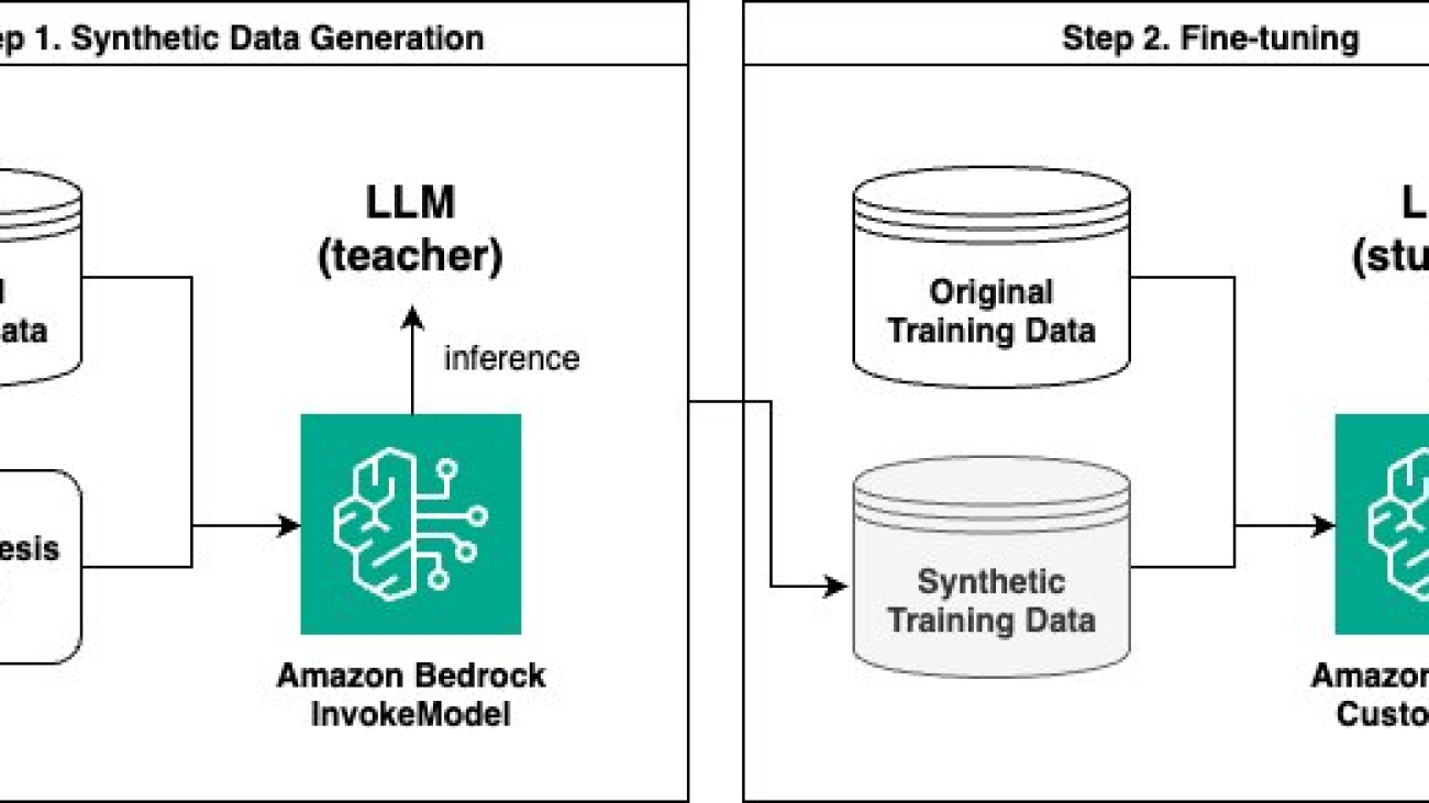
The solution comprises two main steps:
For synthetic data generation, we use a larger language model (such as Anthropic’s Claude 3 Sonnet on Amazon Bedrock) as the teacher model, and a smaller language model (such as Anthropic’s Claude Instant 1.2 or Claude 3 Haiku on Amazon Bedrock) as the student model for fine-tuning. We use the larger teacher model to generate new data based on its knowledge, which is then used to train the smaller student model. This concept is similar to knowledge distillation used in deep learning, except that we’re using the teacher model to generate a new dataset from its knowledge rather than directly modifying the architecture of the student model.
The following diagram illustrates the overall flow of the solution.

Finally, we share our experiment results, where we compare the performance of the model fine-tuned with synthetic data to the baseline (not fine-tuned) model and to a model fine-tuned with an equal amount of original training data.
To generate synthetic data and fine-tune models using Amazon Bedrock, you first need to create an AWS Identity and Access Management (IAM) service role with the appropriate permissions. This role is used by Amazon Bedrock to access the necessary resources on your behalf.
For instructions on creating the service role, refer to Create a service role for model customization. Also, make sure the role has the permission for the bedrock:InvokeModel action.
If you’re running this code using an Amazon SageMaker notebook instance, edit the IAM role that’s attached to the notebook (for example, AmazonSageMaker-ExecutionRole-XXX) instead of creating a new role. Follow Create a service role for model customization to modify the trust relationship and add the S3 bucket permission. Additionally, on the role’s Permissions tab, create the following inline policies:
The final permission policies for the SageMaker execution role should look like the following, which include AmazonSageMaker-ExecutionPolicy, AmazonSageMakerFullAccess, bedrock-customization, and iam-pass-role.

We use the Amazon Bedrock InvokeModel API to generate synthetic data for fine-tuning. You can use the API to programmatically send an inference (text generation) request to the model of your choice. All you need is a well-crafted prompt tailored for data synthesis. We used the following sample prompt for our use case:
The goal of our use case was to fine-tune a model to generate a relevant and coherent answer based on a given reference document and a question. RAG is a popular technique used for such Q&A tasks; however, one significant challenge with RAG is the potential for retrieving unrelated or irrelevant documents, which can lead to inaccurate responses. You can apply fine-tuning to guide the model to better focus on the relevance of the documents to the question instead of using the provided documents without context to answer the question.
Our dataset includes Q&A pairs with reference documents regarding AWS services. Each sample has up to five reference documents as context, and a single-line question follows. The following table shows an example.
| document |
Context: Document 1: Step 1: Prepare to work with AWS CodeStar projects In this step, you create an AWS CodeStar service role and an Amazon EC2 key pair, so that you can begin creating and working with AWS CodeStar projects. If you have used AWS CodeStar before, skip ahead to Step 2 Step 2: Create a Project in AWS CodeStar. For this step, follow the instructions in Setting Up AWS CodeStar in the AWS CodeStar User Guide. Do not create a new AWS account, IAM user, or IAM group as part of those instructions. Use the ones you created or identified in Team Setup for AWS Cloud9. When you finish following those instructions, return to this topic. Document 2: Setting Up AWS CodeStar Before you can start using AWS CodeStar, you must complete the following steps. Topics: Step 1: Create an account Step 2: Create the AWS CodeStar Service Role Step 3: Configure the User’s IAM Permissions Step 4: Create an Amazon EC2 Key Pair for AWS CodeStar Projects Step 5: Open the AWS CodeStar Console Next Steps Document 3: How Do I Get Started with AWS CodeStar? To get started with AWS CodeStar: Prepare to use AWS CodeStar by following the steps in Setting Up AWS CodeStar. Experiment with AWS CodeStar by following the steps in the Getting Started with AWS CodeStar tutorial. Share your project with other developers by following the steps in Add Team Members to an AWS CodeStar Project. Integrate your favorite IDE by following the steps in Use an IDE with AWS CodeStar. Document 4: Step 2: Create a project in AWS CodeStar In this step, you create a project in AWS CodeStar. If you already have a project in AWS CodeStar you want to use, skip ahead to Step 3: Create an AWS Cloud9 Development Environment and Connect It to the Project. For this step, follow the instructions in Create a Project in AWS CodeStar in the AWS CodeStar User Guide. In the AWS CodeStar create project wizard, when you get to the Setup tools page or Connect to your source repository page, choose Skip, and then return to this topic. Document 5: Create a Project in AWS CodeStar You use the AWS CodeStar console to create a project. If you use a project template, it sets up the required resources for you. The template also includes sample code that you can use to start coding. To create a project, sign in to the AWS Management Console with an IAM user that has the AWSCodeStarFullAccess policy or equivalent permissions. For more information, see Setting Up AWS CodeStar. Note: You must complete the steps in Setting Up AWS CodeStar before you can complete the procedures in this topic. Topics Create a Project in AWS CodeStar (Console) Create a Project in AWS CodeStar (AWS CLI) Answer the following question to the best of your ability. Use and paraphrase the information in the context, if it answers the question. Otherwise, rely on your knowledge and memory. |
| question | How do I get started with AWS CodeStar? |
| answer |
To get started with AWS CodeStar, follow these steps: 1. Prepare to work with AWS CodeStar projects: a. Create an AWS CodeStar service role by following the instructions in “Setting Up AWS CodeStar” (Document 2) in the AWS CodeStar User Guide [1]. b. Create an Amazon EC2 key pair for AWS CodeStar projects, as described in the same guide [1]. 2. Create a project in AWS CodeStar: a. Sign in to the AWS Management Console with an IAM user that has the AWSCodeStarFullAccess policy or equivalent permissions [2]. b. In the AWS CodeStar console, select one of the available project templates, which will automatically provision all the required resources for your project [3]. c. Once your project is provisioned, you can see your running application from the Application endpoints tile [3]. 3. Connect to the AWS CodeCommit source repository for your project: a. Use the steps provided in the CodeStar console to connect to the AWS CodeCommit source repository for your project [3]. b. Begin coding and making changes to your project’s source code. 4. Track and manage changes in the release process: a. Use the project dashboard to track and manage changes in the release process [3]. b. View the most recent project activity on the dashboard. 5. Share your project with other developers: a. Follow the steps in “Add Team Members to an AWS CodeStar Project” to share your project with other developers [3]. 6. Integrate your favorite IDE: a. Follow the steps in “Use an IDE with AWS CodeStar” to integrate your preferred Integrated Development Environment (IDE) with AWS CodeStar [3]. [1] https://docs.aws.amazon.com/codestar/latest/userguide/setting-up.html [2] https://docs.aws.amazon.com/codestar/latest/userguide/create-project.html [3] https://docs.aws.amazon.com/codestar/latest/userguide/getting-started.html |
For data synthesis, we asked the model to generate three new Q&A pairs per reference document. However, you can adjust the number as needed. The crucial part is to make the model think deeply about a variety of topics. Because the purpose of generating synthetic data is to enrich the training dataset, it’s more beneficial to have the model look at different parts of the documents and create Q&A pairs with different topics than the original.
The following example shows how to generate synthetic data with the Amazon Bedrock InvokeModel API. We tested the preceding prompt with Anthropic’s Claude 3 Sonnet. If you want to test a different model, retrieve the corresponding model ID from Amazon Bedrock model IDs, and replace the modelId variable in the function.
The preceding function returns three JSONL records in strings with question, answer, and topic as keys. The following parse_llm_output function loads the strings and uses regular expressions to retrieve the generated questions and answers. Then, the create_synthetic_samples function combines those two functionalities to produce the final synthetic training samples.
The following script combines all of the preceding functions and gives you the final training set with both original and synthetic samples. We convert the samples into the format required by the customization job using the to_customization_format function and save them as train.jsonl. Assume the input data is a CSV file with three columns: document, question, and answer.
Now that you have the synthetic data generated by the teacher model along with your original data, it’s time to train the student model. We fine-tune the student model using the Amazon Bedrock custom model functionality.
Model customization is the process of providing training data to an FM to improve its performance for specific use cases. Amazon Bedrock offers three model customization methods as of this writing:
You can create your own custom model using any of these methods through the Amazon Bedrock console or API. For more information on supported models and AWS Regions with various customization methods, please see User guide for model customization. In this section, we focus on how to fine-tune a model using the API.
To create a fine-tuning job in Amazon Bedrock, complete the following prerequisite steps:
When these steps are complete, run the following code to submit a new fine-tuning job. In our use case, the student model was Anthropic’s Claude Instant 1.2. At the time of writing, Anthropic’s Claude 3 Haiku is generally available, and we recommend following the rest of the code using Anthropic’s Claude 3 Haiku. For the release announcement, see Fine-tuning for Anthropic’s Claude 3 Haiku in Amazon Bedrock is now generally available.
If you want to try different models, you must check the model provider’s terms of service yourself. Many providers restrict using their models to train competing models. For the latest model support information, see Supported Regions and models for model customization, and replace baseModelIdentifier accordingly. Different models have different hyperparameters. For more information, see Custom model hyperparameters.
When the status changes to Completed, your fine-tuned student model is ready for use. To run an inference with this custom model, you need to purchase provisioned throughput. A flexible No commitment option is available for custom models, which can be turned off when not in use and billed by the hour. A cost estimate is provided on the console prior to purchasing provisioned throughput.
On the Amazon Bedrock console, choose Custom models in the navigation pane. Select the model you fine-tuned and choose Purchase provisioned throughput.

The model name and type are automatically selected for you. Select No commitment for Commitment term. After you make this selection, the estimated cost is shown. If you’re okay with the pricing, choose Confirm purchase.

When the Provisioned Throughput becomes available, retrieve the ARN of the provisioned custom model and run the inference:
In this section, we share our experiment results to provide data points on how the synthetic data generated by a teacher model can improve the performance of a student model. For evaluation methods, we used an LLM-as-a-judge approach, where a judge model compares responses from two different models and picks a better response. Additionally, we conducted a manual evaluation on a small subset to assess whether the LLM-as-a-judge and human judges have aligned preferences.
We carried out controlled experiments where we compared four different models as follows: 1,500 synthetic training samples for the 4th model were generated by Anthropic’s Claude 3 Sonnet, and we created three synthetic samples per one original reference document (3 samples * 500 original reference documents = 1,500 synthetic samples).
| Instant base model | Anthropic’s Claude Instant without any customization |
| Fine-tuned 500 original | Anthropic’s Claude Instant fine-tuned with 500 original training samples |
| Fine-tuned 2,000 original | Anthropic’s Claude Instant fine-tuned with 2,000 original training samples |
| Fine-tuned with synthetic | Anthropic’s Claude Instant fine-tuned with 500 original training samples plus 1,500 synthetic training samples |
LLM output evaluation is an important step in developing generative AI applications, but it is expensive and takes considerable time if done manually. An alternative solution to systematically evaluate output quality in large volume is the LLM-as-a-judge approach, where an LLM is used to evaluate another LLM’s responses.
For our use case, we used Anthropic’s Claude 3 Sonnet and Meta Llama 3 70B as the judges. We asked the LLM judges to compare outputs from two different models and choose one over the other or state a tie. The following chart summarizes the judges’ decisions. Each number represents the percentage of times when the respective model was selected as providing a better answer, excluding tie cases. The test set contained 343 samples.

As shown in the preceding chart, the Anthropic’s Claude 3 Sonnet judge preferred the response from the fine-tuned model with synthetic examples over the Anthropic’s Claude Instant base model (84.8% preference) and the fine-tuned model with original 500 samples (72.3% preference). However, the judge concluded that the fine-tuned model with 2,000 original examples was preferred over the fine-tuned model with synthetic examples (32.3% preference). This aligns with the expectation that when large, high-quality original data is available, it’s better to use the large training data that accurately reflects the target data distribution.

The Meta Llama judge reached a similar conclusion. As shown in the preceding chart, it preferred the response from the fine-tuned model with synthetic samples over the Anthropic’s Claude Instant base model (75.6% preference) and the fine-tuned model with original 500 examples (76.4% preference), but the fine-tuned model with 2,000 original examples was the ultimate winner.
To complement the LLM-as-a-judge result, we conducted manual evaluation with two human judges. We asked the two human evaluators to perform the same pairwise comparison task as the LLM judge, but for 20 examples. The following chart summarizes the results.

As shown in the preceding chart, the two human evaluators reached a similar conclusion, reinforcing the LLM-as-a-judge result. The fine-tuned model with synthetic examples produced outputs that were more preferable than the Anthropic’s Claude Instant base model and the fine-tuned model with the original 500 examples; however, it didn’t outperform the fine-tuned model with the 2,000 original examples.
These comparative evaluation results from both the LLM judges and human judges strongly demonstrate the power and potential of using data synthesis when training data is scarce. Moreover, by using high-quality data from the teacher model, we can effectively train the student model, which is lightweight and cost-effective for deployment in a production environment.
Running LLM-as-a-judge and human evaluation has become much easier with Amazon Bedrock. Model evaluation on Amazon Bedrock allows you to evaluate, compare, and select the best FMs for your use case. Human evaluation workflows can use your own employees or an AWS-managed team as reviewers. For more information on how to set up a human evaluation workflow, see Creating your first model evaluation that uses human workers. The latest feature, LLM-as-a-judge, is now in preview and allows you to assess multiple quality dimensions including correctness, helpfulness, and responsible AI criteria such as answer refusal and harmfulness. For step-by-step instructions, see New RAG evaluation and LLM-as-a-judge capabilities in Amazon Bedrock.
Make sure to delete the following resources to avoid incurring cost:
In this post, we explored how to use Amazon Bedrock to generate synthetic training data using a large teacher language model and fine-tune a smaller student model with synthetic data. We provided instructions on generating synthetic data using the Amazon Bedrock InvokeModel API and fine-tuning the student model using an Amazon Bedrock custom model. Our evaluation results, based on both an LLM-as-a-judge approach and human evaluation, demonstrated the effectiveness of synthetic data in improving the student model’s performance when original training data is limited.
Although fine-tuning with a large amount of high-quality original data remains the ideal approach, our findings highlight the promising potential of synthetic data generation as a viable solution when dealing with data scarcity. This technique can enable more efficient and cost-effective model customization for domain-specific or specialized use cases.
If you’re interested in working with the AWS Generative AI Innovation Center and learning more about LLM customization and other generative AI use cases, visit Generative AI Innovation Center.
 Sujeong Cha is a Deep Learning Architect at the AWS Generative AI Innovation Center, where she specializes in model customization and optimization. She has extensive hands-on experience in solving customers’ business use cases by utilizing generative AI as well as traditional AI/ML solutions. Sujeong holds a M.S. degree in Data Science from New York University.
 Arijit Ghosh Chowdhury is a Scientist with the AWS Generative AI Innovation Center, where he works on model customization and optimization. In his role, he works on applied research in fine-tuning and model evaluations to enable GenAI for various industries. He has a Master’s degree in Computer Science from the University of Illinois at Urbana Champaign, where his research focused on question answering, search and domain adaptation.
 Sungmin Hong is a Senior Applied Scientist at Amazon Generative AI Innovation Center where he helps expedite the variety of use cases of AWS customers. Before joining Amazon, Sungmin was a postdoctoral research fellow at Harvard Medical School. He holds Ph.D. in Computer Science from New York University. Outside of work, Sungmin enjoys hiking, reading and cooking.
 Yiyue Qian is an Applied Scientist II at the AWS Generative AI Innovation Center, where she develops generative AI solutions for AWS customers. Her expertise encompasses designing and implementing innovative AI-driven and deep learning techniques, focusing on natural language processing, computer vision, multi-modal learning, and graph learning. Yiyue holds a Ph.D. in Computer Science from the University of Notre Dame, where her research centered on advanced machine learning and deep learning methodologies. Outside of work, she enjoys sports, hiking, and traveling.
 Wei-Chih Chen is a Machine Learning Engineer at the AWS Generative AI Innovation Center, where he works on model customization and optimization for LLMs. He also builds tools to help his team tackle various aspects of the LLM development life cycle—including fine-tuning, benchmarking, and load-testing—that accelerating the adoption of diverse use cases for AWS customers. He holds an M.S. degree in Computer Science from UC Davis.
 Hannah Marlowe is a Senior Manager of Model Customization at the AWS Generative AI Innovation Center. Her team specializes in helping customers develop differentiating Generative AI solutions using their unique and proprietary data to achieve key business outcomes. She holds a Ph.D in Physics from the University of Iowa, with a focus on astronomical X-ray analysis and instrumentation development. Outside of work, she can be found hiking, mountain biking, and skiing around the mountains in Colorado.
This blog post is co-written with Moran beladev, Manos Stergiadis, and Ilya Gusev from Booking.com.
Large language models (LLMs) have revolutionized the field of natural language processing with their ability to understand and generate humanlike text. Trained on broad, generic datasets spanning a wide range of topics and domains, LLMs use their parametric knowledge to perform increasingly complex and versatile tasks across multiple business use cases. Furthermore, companies are increasingly investing resources in customizing LLMs through few-shot learning and fine-tuning to optimize their performance for specialized applications.
However, the impressive performance of LLMs comes at the cost of significant computational requirements, driven by their large number of parameters and autoregressive decoding process which is sequential in nature. This combination makes achieving low latency a challenge for use cases such as real-time text completion, simultaneous translation, or conversational voice assistants, where subsecond response times are critical.
Researchers developed Medusa, a framework to speed up LLM inference by adding extra heads to predict multiple tokens simultaneously. This post demonstrates how to use Medusa-1, the first version of the framework, to speed up an LLM by fine-tuning it on Amazon SageMaker AI and confirms the speed up with deployment and a simple load test. Medusa-1 achieves an inference speedup of around two times without sacrificing model quality, with the exact improvement varying based on model size and data used. In this post, we demonstrate its effectiveness with a 1.8 times speedup observed on a sample dataset.
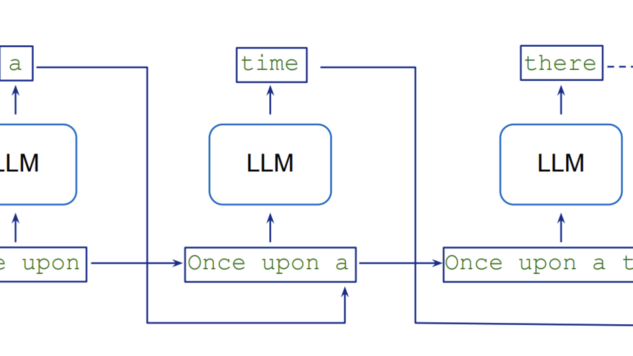
LLMs generate text in a sequential manner, which involves autoregressive sampling, with each new token conditional on the previous ones. Generating K tokens necessitates K sequential executions of the model. This token-by-token processing introduces an inherent latency and computational overhead because the model needs to perform a separate forward pass for each new token in the output sequence. The following diagram from Role-Play with Large Language Models illustrates this flow.

Speculative decoding tackles this challenge by using a smaller, faster draft model to generate multiple potential token continuations in parallel, which are then verified by a larger, more accurate target model. This parallelization speeds up text generation while maintaining the quality of the target model because the verification task is faster than autoregressive token generation. For a detailed explanation of the concept, refer to the paper Accelerating Large Language Model Decoding with Speculative Sampling. The speculative decoding technique can be implemented using the inference optimization toolkit on Amazon SageMaker Jumpstart.
The paper Medusa: Simple LLM Inference Acceleration Framework with Multiple Decoding Heads introduced Medusa as an alternative to speculative decoding. Instead of adding a separate draft model, it adds extra decoding heads to the LLM that generate candidate continuations simultaneously. These candidates are then evaluated in parallel using a tree-based attention mechanism. This parallel processing reduces the number of sequential steps needed, leading to faster inference times. The main advantage of Medusa over speculative decoding is that it eliminates the need to acquire and maintain a separate draft model while achieving higher speedups. For example, when tested on the MT-Bench dataset, the paper reports that Medusa-2 (the second version of Medusa) speeds up inference time by 2.8 times. This outperforms speculative decoding, which only manages to speed up inference time by 1.5 times on the same dataset.
The Medusa framework currently supports Llama and Mistral models. Although it offers significant speed improvements, it does come with a memory trade-off (similar to speculative decoding). For instance, adding five Medusa heads to the 7-billion-parameter Mistral model increases the total parameter count by 750 million (150 million per head), which means these additional parameters must be stored in GPU memory, leading to a higher memory requirement. However, in most cases, this increase doesn’t necessitate switching to a higher GPU memory instance. For example, you can still use an ml.g5.4xlarge instance with 24 GB of GPU memory to host your 7-billion-parameter Llama or Mistral model with extra Medusa heads.
Training Medusa heads requires additional development time and computational resources, which should be factored into project planning and resource allocation. Another important limitation to mention is that the current framework, when deployed on an Amazon SageMaker AI endpoint, only supports a batch size of one—a configuration typically used for low-latency applications.
The following diagram from the original Medusa paper authors’ FasterDecoding repository gives a visual Medusa framework overview.

There are two main variants of Medusa:
The Medusa paper reports that across models of varying sizes, you can achieve inference speedups of around two times for Medusa-1 and around three times for Medusa-2. With Medusa-1, the predictions are identical to those of the originally fine-tuned LLM. In contrast, with Medusa-2, we might observe slightly different results compared to simple fine-tuning of the LLM because both the heads and the backbone LLM parameters are updated together. In this post, we focus on Medusa-1.
We cover the following steps in our solution:
By following this solution, you can accelerate LLM inference in your applications, leading to faster response times and improved user experience.
To build the solution yourself, there are the following prerequisites:
AmazonSageMakerFullAccess and AmazonS3FullAccess). For details, refer to Creating an AWS account.ml.t3.medium instance with a Python 3 (ipykernel) kernel. However, you can also use an Amazon SageMaker notebook instance (with a conda_pytorch_p310 kernel) or any integrated development environment (IDE) of your choice.ml.g5.4xlarge instance for the SageMaker AI training jobs, and three ml.g5.4xlarge instance are used for the SageMaker AI endpoints. Make sure you have sufficient capacity for this instance in your AWS account by requesting a quota increase if required. Also check the pricing of the on-demand instances to understand the associated costs.medusa_1_train.ipynb notebook to run all the steps in this post. This repository is a modified version of the original How to Fine-Tune LLMs in 2024 on Amazon SageMaker. We added simplified Medusa training code, adapted from the original Medusa repository.Now that you have cloned the GitHub repository and opened the medusa_1_train.ipynb notebook, you will load and prepare the dataset in the notebook. We encourage you to read this post while running the code in the notebook. For this post, we use a dataset called sql-create-context, which contains samples of natural language instructions, schema definitions and the corresponding SQL query. It contains 78,577 examples of natural language queries, SQL CREATE TABLE statements, and SQL queries answering the question using the CREATE statement as context. For demonstration purposes, we select 3,000 samples and split them into train, validation, and test sets.
You need to run the “Load and prepare the dataset” section of the medusa_1_train.ipynb to prepare the dataset for fine-tuning. We also included a data exploration script to analyze the length of input and output tokens. After data exploration, we prepare the train, validation, and test sets and upload them to Amazon Simple Storage Service (Amazon S3).
We use the Zephyr 7B β model as our backbone LLM. Zephyr is a series of language models trained to act as helpful assistants, and Zephyr 7B β is a fine-tuned version of Mistral-7B-v0.1, trained on a mix of publicly available and synthetic datasets using Direct Preference Optimization.
To launch a SageMaker AI training job, we need to use the PyTorch or Hugging Face estimator. SageMaker AI starts and manages all the necessary Amazon Elastic Compute Cloud (Amazon EC2) instances for us, supplies the appropriate containers, downloads data from our S3 bucket to the container and uploads and runs the specified training script, in our case fine_tune_llm.py. We select the hyperparameters based on the QLoRA paper, but we encourage you to experiment with your own combinations. To expedite the execution of this code, we set the number of epochs to 1. However, for better results, it’s generally recommended to set the number of epochs to at least 2 or 3.
When our training job has completed successfully after approximately 1 hour, we can use the fine-tuned model artifact for the next step, training the Medusa heads on top of it. To visualize the training metrics in Tensorboard, you can follow the guidance in this documentation: Load and visualize output tensors using the TensorBoard application
For training Medusa heads, we can reuse the functions previously mentioned to launch the training job. We selected hyperparameters based on a combination of what the Medusa paper reported and what we found to be best performing after a few experiments. We set the number of Medusa heads to 5 and used the 8-bit AdamW optimizer, as recommended by the paper. For simplicity, we maintained a constant learning rate of 1e-4 with a constant scheduler, similar to the previous fine-tuning step. Although the paper recommends an increased learning rate and a cosine scheduler, we found that our chosen combination of hyperparameters performed well on this dataset. However, we encourage you to experiment with your own hyperparameter settings to potentially achieve even better results.
We found that after 3 epochs, the evaluation loss of Medusa heads was converging, which can be observed in the TensorBoard graph in the following image.

Besides the hyperparameters, the main difference is that we pass train_medusa_heads.py as the training entrypoint, where we first add Medusa heads, then freeze the fine-tuned LLM, and we create custom MedusaSFTTrainer class, which is a subclass of the transformers SFTTrainer.
In the add_medusa_heads() function, we add the residual blocks of the Medusa heads, and also override the forward pass for our model to make sure not to train the frozen backbone LLM:
After the model training is finished (which takes 1 hour), we prepare the model artefacts for deployment and upload it to Amazon S3. Your final model artifact contains both the original fine-tuned model from the previous step under the base-model prefix and the trained Medusa heads in a file named medusa_heads.safetensors.
The Medusa framework is supported by the Text Generation Inference (TGI) server. After training the LLM with Medusa heads, we deploy it to a SageMaker AI real-time endpoint using the Hugging Face Inference Container set up with TGI.
First, we create a SageMaker AI HuggingFaceModel object and then deploy the model to an endpoint with the following function:
We deploy three LLMs on three SageMaker AI endpoints:
You can deploy the three models in parallel by using a function that we included in the notebook, or you can deploy the models one by one by running the code below:
After the status for each endpoint becomes InService, which should take around 15 minutes, we can invoke them for inference. We send the following input:
We can observe the following responses:
To measure the inference speed improvements, we compare the response times of the deployed fine-tuned LLM and the fine-tuned LLM with Medusa heads on 450 test observations with the following code:
First, we run predictions using the fine-tuned LLM:
Then, we run predictions using the fine-tuned LLM with Medusa heads:
The prediction runs should take around 8 and 4 minutes respectively. We can observe that the average latency decreased from 950 to 530 milliseconds, which is an improvement of 1.8 times. You can achieve even higher improvements if your dataset contains longer inputs and outputs. In our dataset, we only had an average of 18 input tokens and 30 output tokens.
We want to once again highlight that, with this technique, the output quality is fully maintained, and all the prediction outputs are the same. The model responses for the test set of 450 observations are the same for both with Medusa heads and without Medusa heads:
You might notice in your run that a few observations aren’t exactly matching, and you might get a 99% match due to small errors in floating point operations caused by optimizations on GPUs.
At the end of this experiment, don’t forget to delete the SageMaker AI endpoints you created:
In this post, we demonstrated how to fine-tune and deploy an LLM with Medusa heads using the Medusa-1 technique on Amazon SageMaker AI to accelerate LLM inference. By using this framework and SageMaker AI scalable infrastructure, we showed how to achieve up to twofold speedups in LLM inference while maintaining model quality. This solution is particularly beneficial for applications requiring low-latency text generation, such as customer service chat assistants, content creation, and recommendation systems.
As a next step, you can explore fine-tuning your own LLM with Medusa heads on your own dataset and benchmark the results for your specific use case, using the provided GitHub repository.
 Daniel Zagyva is a Senior ML Engineer at AWS Professional Services. He specializes in developing scalable, production-grade machine learning solutions for AWS customers. His experience extends across different areas, including natural language processing, generative AI and machine learning operations.
 Aleksandra Dokic is a Senior Data Scientist at AWS Professional Services. She enjoys supporting customers to build innovative AI/ML solutions on AWS and she is excited about business transformations through the power of data.
 Moran Beladev is a Senior ML Manager at Booking.com. She is leading the content intelligence track which is focused on building, training and deploying content models (computer vision, NLP and generative AI) using the most advanced technologies and models. Moran is also a PhD candidate, researching applying NLP models on social graphs.
 Manos Stergiadis is a Senior ML Scientist at Booking.com. He specializes in generative NLP and has experience researching, implementing and deploying large deep learning models at scale.
 Ilya Gusev is a Senior Machine Learning Engineer at Booking.com. He leads the development of the several LLM systems inside Booking.com. His work focuses on building production ML systems that help millions of travelers plan their trips effectively.
 Laurens van der Maas is a Machine Learning Engineer at AWS Professional Services. He works closely with customers building their machine learning solutions on AWS, specializes in natural language processing, experimentation and responsible AI, and is passionate about using machine learning to drive meaningful change in the world.

The evaluation of large language model (LLM) performance, particularly in response to a variety of prompts, is crucial for organizations aiming to harness the full potential of this rapidly evolving technology. The introduction of an LLM-as-a-judge framework represents a significant step forward in simplifying and streamlining the model evaluation process. This approach allows organizations to assess their AI models’ effectiveness using pre-defined metrics, making sure that the technology aligns with their specific needs and objectives. By adopting this method, companies can more accurately gauge the performance of their AI systems, making informed decisions about model selection, optimization, and deployment. This not only enhances the reliability and efficiency of AI applications, but also contributes to a more strategic and informed approach to technology adoption within the organization.
Amazon Bedrock, a fully managed service offering high-performing foundation models from leading AI companies through a single API, has recently introduced two significant evaluation capabilities: LLM-as-a-judge under Amazon Bedrock Model Evaluation and RAG evaluation for Amazon Bedrock Knowledge Bases. Both features use the LLM-as-a-judge technique behind the scenes but evaluate different things. This blog post explores LLM-as-a-judge on Amazon Bedrock Model Evaluation, providing comprehensive guidance on feature setup, evaluating job initiation through both the console and Python SDK and APIs, and demonstrating how this innovative evaluation feature can enhance generative AI applications across multiple metric categories including quality, user experience, instruction following, and safety.
Before we explore the technical aspects and implementation details, let’s examine the key features that make LLM-as-a-judge on Amazon Bedrock Model Evaluation particularly powerful and distinguish it from traditional evaluation methods. Understanding these core capabilities will help illuminate why this feature represents a significant advancement in AI model evaluation.
These features create a powerful evaluation framework that helps organizations optimize their AI model performance while maintaining high standards of quality and safety, all within their secure AWS environment.
Now that you understand the key features of LLM-as-a-judge, let’s examine how to implement and use this capability within Amazon Bedrock Model Evaluation. This section provides a comprehensive overview of the architecture and walks through each component, demonstrating how they work together to deliver accurate and efficient model evaluations.
LLM-as-a-judge on Amazon Bedrock Model Evaluation provides a comprehensive, end-to-end solution for assessing and optimizing AI model performance. This automated process uses the power of LLMs to evaluate responses across multiple metric categories, offering insights that can significantly improve your AI applications. Let’s walk through the key components of this solution as shown in the following diagram:

LLM-as-a-judge on Amazon Bedrock Model Evaluation follows a streamlined workflow that enables systematic model evaluation. Here’s how each component works together in the evaluation process:
With this solution architecture in mind, let’s explore how to implement LLM-as-a-judge model evaluations effectively, making sure that you get the most valuable insights from your assessment process.
To use the LLM-as-a-judge model evaluation, make sure that you have satisfied the following requirements:
When preparing your dataset for LLM-as-a-judge model evaluation jobs, each prompt must include specific key-value pairs. Here are the required and optional fields:
Dataset requirements:
Example JSONL format without ground truth (category is optional):
Example JSONL format with ground truth (category is optional):
You can use LLM-as-a-judge on Amazon Bedrock Model Evaluation to assess model performance through a user-friendly console interface. Follow these steps to start an evaluation job:


To use the Python SDK for creating an LLM-as-a-judge model evaluation job, use the following steps. First, set up the required configurations:
To create an LLM-as-a-judge model evaluation job:
To monitor the progress of your evaluation job:
You can also compare multiple foundation models to determine which one works best for your needs. By using the same evaluator model across all comparisons, you’ll get consistent benchmarking results to help identify the optimal model for your use case.
You can use the Spearman’s rank correlation coefficient to compare evaluation results between different generator models using LLM-as-a-judge in Amazon Bedrock. After retrieving the evaluation results from your S3 bucket, containing evaluation scores across various metrics, you can begin the correlation analysis.
Using scipy.stats, compute the correlation coefficient between pairs of generator models, filtering out constant values or error messages to have a valid statistical comparison. The resulting correlation coefficients help identify how similarly different models respond to the same prompts. A coefficient closer to 1.0 indicates stronger agreement between the models’ responses, while values closer to 0 suggest more divergent behavior. This analysis provides valuable insights into model consistency and helps identify cases where different models might produce significantly different outputs for the same input.
You can also compare multiple foundation models to determine which one works best for your needs. By using the same evaluator model across all comparisons, you’ll get consistent, scalable results. The following best practices will help you establish standardized benchmarking when comparing different foundation models.
These best practices help establish a robust evaluation framework using LLM-as-a-judge on Amazon Bedrock. For deeper insights into the scientific validation of these practices, including case studies and correlation with human judgments, stay tuned for our upcoming technical deep-dive blog post.
LLM-as-a-judge on Amazon Bedrock Model Evaluation represents a significant advancement in automated model assessment, offering organizations a powerful tool to evaluate and optimize their AI applications systematically. This feature combines the efficiency of automated evaluation with the nuanced understanding typically associated with human assessment, enabling organizations to scale their quality assurance processes while maintaining high standards of performance and safety.
The comprehensive metric categories, flexible implementation options, and seamless integration with existing AWS services make it possible for organizations to establish robust evaluation frameworks that grow with their needs. Whether you’re developing conversational AI applications, content generation systems, or specialized enterprise solutions, LLM-as-a-judge provides the necessary tools to make sure that your models align with both technical requirements and business objectives.
We’ve provided detailed implementation guidance, from initial setup to best practices, to help you use this feature effectively. The accompanying code samples and configuration examples in this post demonstrate how to implement these evaluations in practice. Through systematic evaluation and continuous improvement, organizations can build more reliable, accurate, and trustworthy AI applications.
We encourage you to explore LLM-as-a-judge capabilities in the Amazon Bedrock console and discover how automatic evaluation can enhance your AI applications. To help you get started, we’ve prepared a Jupyter notebook with practical examples and code snippets that you can find on our GitHub repository.
 Adewale Akinfaderin is a Sr. Data Scientist–Generative AI, Amazon Bedrock, where he contributes to cutting edge innovations in foundational models and generative AI applications at AWS. His expertise is in reproducible and end-to-end AI/ML methods, practical implementations, and helping global customers formulate and develop scalable solutions to interdisciplinary problems. He has two graduate degrees in physics and a doctorate in engineering.
 Ishan Singh is a Generative AI Data Scientist at Amazon Web Services, where he helps customers build innovative and responsible generative AI solutions and products. With a strong background in AI/ML, Ishan specializes in building Generative AI solutions that drive business value. Outside of work, he enjoys playing volleyball, exploring local bike trails, and spending time with his wife and dog, Beau.
 Jesse Manders is a Senior Product Manager on Amazon Bedrock, the AWS Generative AI developer service. He works at the intersection of AI and human interaction with the goal of creating and improving generative AI products and services to meet our needs. Previously, Jesse held engineering team leadership roles at Apple and Lumileds, and was a senior scientist in a Silicon Valley startup. He has an M.S. and Ph.D. from the University of Florida, and an MBA from the University of California, Berkeley, Haas School of Business.
Generative AI has emerged as a transformative force, captivating industries with its potential to create, innovate, and solve complex problems. However, the journey from a proof of concept to a production-ready application comes with challenges and opportunities. Moving from proof of concept to production is about creating scalable, reliable, and impactful solutions that can drive business value and user satisfaction.
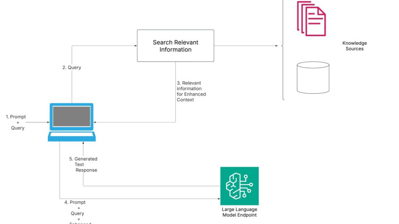
One of the most promising developments in this space is the rise of Retrieval Augmented Generation (RAG) applications. RAG is the process of optimizing the output of a foundation model (FM), so it references a knowledge base outside of its training data sources before generating a response.
The following diagram illustrates a sample architecture.

In this post, we explore the movement of RAG applications from their proof of concept or minimal viable product (MVP) phase to full-fledged production systems. When transitioning a RAG application from a proof of concept to a production-ready system, optimization becomes crucial to make sure the solution is reliable, cost-effective, and high-performing. Let’s explore these optimization techniques in greater depth, setting the stage for future discussions on hosting, scaling, security, and observability considerations.
The diagram below illustrates the tradeoffs to consider for a production-ready RAG application.

The success of a production-ready RAG system is measured by its quality, cost, and latency. Machine learning (ML) engineers must make trade-offs and prioritize the most important factors for their specific use case and business requirements. For example, consider the use case of generating personalized marketing content for a luxury fashion brand. The brand might be willing to absorb the higher costs of using a more powerful and expensive FMs to achieve the highest-quality classifications, because misclassifications could lead to customer dissatisfaction and damage the brand’s reputation. Consider another use case of generating personalized product descriptions for an ecommerce site. The retailer might be willing to accept slightly longer latency to reduce infrastructure and operational costs, as long as the generated descriptions remain reasonably accurate and compelling. The optimal balance of quality, cost, and latency can vary significantly across different applications and industries.
Let’s look into practical guidelines on how you can enhance the overall quality of your RAG workflow, including the quality of the retriever and quality of the result generator using Amazon Bedrock Knowledge Bases and other features of Amazon Bedrock. Amazon Bedrock Knowledge Bases provides a fully managed capability that helps you implement the entire RAG workflow from ingestion to retrieval and prompt augmentation without having to build custom integrations to data sources and manage data flows.
An effective evaluation framework is crucial for assessing and optimizing RAG systems as they move from proof of concept to production. These frameworks typically include overall metrics for a holistic assessment of the entire RAG pipeline, as well as specific diagnostic metrics for both the retrieval and generation components. This allows for targeted improvements in each phase of the system. By implementing a robust evaluation framework, developers can continuously monitor, diagnose, and enhance their RAG systems, achieving optimal performance across quality, cost, and latency dimensions as the application scales to production levels. Amazon Bedrock Evaluations can help you evaluate your retrieval or end-to-end RAG workflow in Amazon Bedrock Knowledge Bases. In the following sections, we discuss these specific metrics in different phases of the RAG workflow in more detail.
For better retrieval performance, the way the data is stored in the vector store has a big impact. For example, your input document might include tables within the PDF. In such cases, using an FM to parse the data will provide better results. You can use advanced parsing options supported by Amazon Bedrock Knowledge Bases for parsing non-textual information from documents using FMs. Many organizations store their data in structured formats within data warehouses and data lakes. Amazon Bedrock Knowledge Bases offers a feature that lets you connect your RAG workflow to structured data stores. This fully managed out-of-the-box RAG solution can help you natively query structured data from where it resides.
Another important consideration is the way your source document is split up into chunks. If your document would benefit from inherent relationships within your document, it might be wise to use hierarchical chunking, which allows for more granular and efficient retrieval. Some documents benefit from semantic chunking by preserving the contextual relationship in the chunks, helping make sure that the related information stays together in logical chunks. You can also use your own custom chunking strategy for your RAG application’s unique requirements.
RAG applications process user queries by searching across a large set of documents. However, in many situations, you might need to retrieve documents with specific attributes or content. You can use metadata filtering to narrow down search results by specifying inclusion and exclusion criteria. Amazon Bedrock Knowledge Bases now also supports auto generated query filters, which extend the existing capability of manual metadata filtering by allowing you to narrow down search results without the need to manually construct complex filter expressions. This improves retrieval accuracy by making sure the documents are relevant to the query.
Writing an effective query is just as important as any other consideration for generation accuracy. You can add a prompt providing instructions to the FM to provide an appropriate answer to the user. For example, a legal tech company would want to provide instructions to restrict the answers to be based on the input documents and not based on general information known to the FM. Query decomposition by splitting the input query into multiple queries is also helpful in retrieval accuracy. In this process, the subqueries with less semantic complexity might find more targeted chunks. These chunks can then be pooled and ranked together before passing them to the FM to generate a response.
Reranking, as a post-retrieval step, can significantly improve response quality. This technique uses LLMs to analyze the semantic relevance between the query and retrieved documents, reordering them based on their pertinence. By incorporating reranking, you make sure that only the most contextually relevant information is used for generation, leading to more accurate and coherent responses.
Adjusting inference parameters, such as temperature and top-k/p sampling, can help in further refining the output.
You can use Amazon Bedrock Knowledge Bases to configure and customize queries and response generation. You can also improve the relevance of your query responses with a reranker model in Amazon Bedrock.
The key metrics for retriever quality are context precision, context recall, and context relevance. Context precision measures how well the system ranks relevant pieces of information from the given context. It considers the question, ground truth, and context. Context recall provides the percentage of ground truth claims or key information covered by the retrieved context. Context relevance measures whether the retrieved passages or chunks are relevant for answering the given query, excluding extraneous details. Together, these three metrics offer insight into how effectively the retriever is able to surface the most relevant and focused source material to support a high-quality response.
Generator quality can be assessed through several key metrics. Context utilization examines how effectively the generator uses relevant information from the provided source material. Noise sensitivity gauges the generator’s propensity to include inaccurate details from the retrieved content. Hallucination measures the extent to which the generator produces incorrect claims not present in the source data. Self-knowledge reflects the proportion of accurate statements generated that can’t be found in the retrieved chunks. Finally, faithfulness evaluates how closely the generator’s output aligns with the information contained in the source material.
For measuring the overall generation quality, the key metrics include measuring the precision, recall, and answer similarity. Precision suggests the proportion of the correct claims in model’s response, whereas recall suggests the proportion of the ground truth claims covered by the model’s response. Answer similarity compares the meaning and content of a generated answer with a reference or ground truth answer. It evaluates how closely the generated answer matches the intended meaning of the ground truth answer.
Establishing a feedback loop with an evaluation framework against these quality metrics allows for continuous improvement, where the system can learn from user interactions and refine its performance over time. By optimizing these quality metrics, the RAG system can be designed to deliver reliable, cost-effective, and high-performing results for users.
For a demonstration on how you can use a RAG evaluation framework in Amazon Bedrock to compute RAG quality metrics, refer to New RAG evaluation and LLM-as-a-judge capabilities in Amazon Bedrock.
Implementing responsible AI practices is crucial for maintaining ethical and safe deployment of RAG systems. This includes using guardrails to filter harmful content, deny certain topics, mask sensitive information, and ground responses in verified sources to reduce hallucinations.
You can use Amazon Bedrock Guardrails for implementing responsible AI policies. Along with protecting against toxicity and harmful content, it can also be used for Automated Reasoning checks, which helps you protect against hallucinations.
Cost considers the compute resources and infrastructure required to run the system, and latency evaluates the response times experienced by end-users. To optimize cost and latency, implement caching strategies to reduce the need for expensive model inferences. Efficient query batching can also improve overall throughput and reduce resource usage. Balance performance and resource usage to find the ideal configuration that meets your application’s requirements.
Use tools like Amazon Bedrock Knowledge Bases so you can take advantage of fully managed support for the end-to-end RAG workflow. It supports many of the advanced RAG capabilities we discussed earlier. By addressing these optimization techniques, you can transition your RAG-powered proof of concept to a robust, production-ready system that delivers high-quality, cost-effective, and low-latency responses to your users.
For more information on building RAG applications using Amazon Bedrock Knowledge Bases, refer to Building scalable, secure, and reliable RAG applications using Amazon Bedrock Knowledge Bases.
When it comes to hosting your web application or service, there are several approaches to consider. The key is to choose a solution that can effectively host your database and compute infrastructure. This could include server-based options like Amazon Elastic Compute Cloud (Amazon EC2), managed services like Amazon Relational Database Service (Amazon RDS) and Amazon DynamoDB, or serverless approaches such as AWS Amplify and Amazon Elastic Container Service (Amazon ECS). For a practical approach to building an automated AI assistant using Amazon ECS, see Develop a fully automated chat-based assistant by using Amazon Bedrock agents and knowledge bases.
In addition to the server or compute layer, you will also need to consider an orchestration tool, testing environments, and a continuous integration and delivery (CI/CD) pipeline to streamline your application deployment. Having a feedback loop established based on the quality metrics along with a CI/CD pipeline is an important first step to creating self-healing architectures.
As your application grows, you will need to make sure your infrastructure can scale to meet the increasing demand. This can involve containerization with Docker or choosing serverless options, implementing load balancing, setting up auto scaling, and choosing between on-premises, cloud, or hybrid solutions. It also includes unique scaling requirements of your frontend application and backend generative AI workflow, as well as the use of content delivery networks (CDNs) and disaster recovery and backup strategies.
The following is a sample architecture for a secure and scalable RAG-based web application. This architecture uses Amazon ECS for hosting the service, Amazon CloudFront as a CDN, AWS WAF as a firewall, and Amazon MemoryDB for providing a semantic cache.

By carefully considering these aspects of hosting and scaling your infrastructure, you can build a resilient and adaptable system to support your growing web application or service. Stay tuned for more detailed information on these topics in upcoming blog posts.
Maintaining data privacy and security is of utmost importance. This includes implementing security measures at each layer of your application, from encrypting data in transit to setting up robust authentication and authorization controls. It also involves focusing on compute and storage security, as well as network security. Compliance with relevant regulations and regular security audits are essential. Securing your generative AI system is another crucial aspect. By default, Amazon Bedrock Knowledge Bases encrypts the traffic using AWS managed AWS Key Management Service (AWS KMS) keys. You can also choose customer managed KMS keys for more control over encryption keys. For more information on application security, refer to Safeguard a generative AI travel agent with prompt engineering and Amazon Bedrock Guardrails.
Comprehensive logging, monitoring, and maintenance are crucial to maintaining a healthy infrastructure. This includes setting up structured logging, centralized log management, real-time monitoring, and strategies for system updates and migrations.
By addressing these critical areas, you can build a secure and resilient infrastructure to support your growing web application or service. Stay tuned for more in-depth coverage of these topics in upcoming blog posts.
To successfully transition a RAG application from a proof of concept to a production-ready system, you should focus on optimizing the solution for reliability, cost-effectiveness, and high performance. Key areas to address include enhancing retriever and generator quality, balancing cost and latency, and establishing a robust and secure infrastructure.
By using purpose-built tools like Amazon Bedrock Knowledge Bases to streamline the end-to-end RAG workflow, organizations can successfully transition their RAG-powered proofs of concept into high-performing, cost-effective, secure production-ready solutions that deliver business value.
 Vivek Mittal is a Solution Architect at Amazon Web Services, where he helps organizations architect and implement cutting-edge cloud solutions. With a deep passion for Generative AI, Machine Learning, and Serverless technologies, he specializes in helping customers harness these innovations to drive business transformation. He finds particular satisfaction in collaborating with customers to turn their ambitious technological visions into reality.
 Nitin Eusebius is a Sr. Enterprise Solutions Architect at AWS, experienced in Software Engineering, Enterprise Architecture, and AI/ML. He is deeply passionate about exploring the possibilities of generative AI. He collaborates with customers to help them build well-architected applications on the AWS platform, and is dedicated to solving technology challenges and assisting with their cloud journey.
 Mani Khanuja is a Tech Lead – Generative AI Specialists, author of the book Applied Machine Learning and High-Performance Computing on AWS, and a member of the Board of Directors for Women in Manufacturing Education Foundation Board. She leads machine learning projects in various domains such as computer vision, natural language processing, and generative AI. She speaks at internal and external conferences such AWS re:Invent, Women in Manufacturing West, YouTube webinars, and GHC 23. In her free time, she likes to go for long runs along the beach.
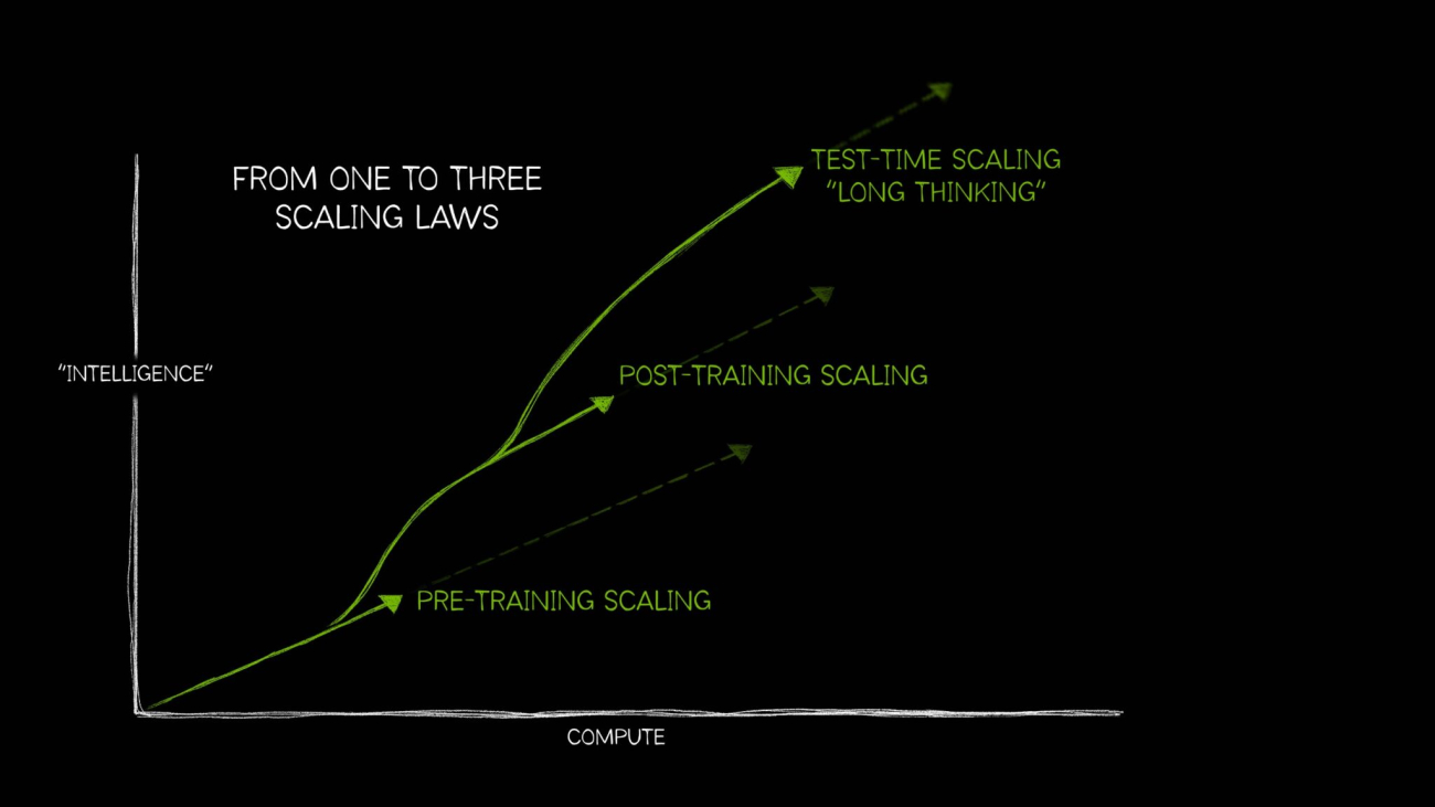
Just as there are widely understood empirical laws of nature — for example, what goes up must come down, or every action has an equal and opposite reaction — the field of AI was long defined by a single idea: that more compute, more training data and more parameters makes a better AI model.
However, AI has since grown to need three distinct laws that describe how applying compute resources in different ways impacts model performance. Together, these AI scaling laws — pretraining scaling, post-training scaling and test-time scaling, also called long thinking — reflect how the field has evolved with techniques to use additional compute in a wide variety of increasingly complex AI use cases.
The recent rise of test-time scaling — applying more compute at inference time to improve accuracy — has enabled AI reasoning models, a new class of large language models (LLMs) that perform multiple inference passes to work through complex problems, while describing the steps required to solve a task. Test-time scaling requires intensive amounts of computational resources to support AI reasoning, which will drive further demand for accelerated computing.
Pretraining scaling is the original law of AI development. It demonstrated that by increasing training dataset size, model parameter count and computational resources, developers could expect predictable improvements in model intelligence and accuracy.
Each of these three elements — data, model size, compute — is interrelated. Per the pretraining scaling law, outlined in this research paper, when larger models are fed with more data, the overall performance of the models improves. To make this feasible, developers must scale up their compute — creating the need for powerful accelerated computing resources to run those larger training workloads.
This principle of pretraining scaling led to large models that achieved groundbreaking capabilities. It also spurred major innovations in model architecture, including the rise of billion- and trillion-parameter transformer models, mixture of experts models and new distributed training techniques — all demanding significant compute.
And the relevance of the pretraining scaling law continues — as humans continue to produce growing amounts of multimodal data, this trove of text, images, audio, video and sensor information will be used to train powerful future AI models.
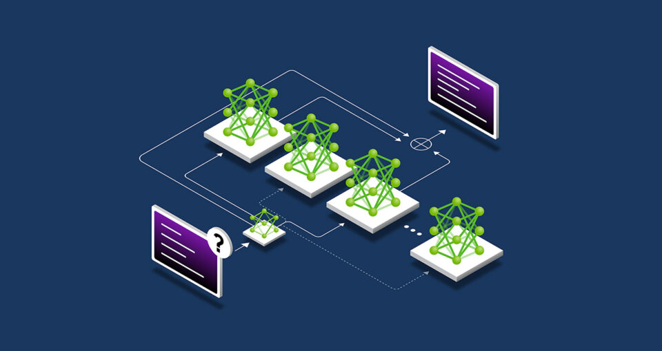
Pretraining a large foundation model isn’t for everyone — it takes significant investment, skilled experts and datasets. But once an organization pretrains and releases a model, they lower the barrier to AI adoption by enabling others to use their pretrained model as a foundation to adapt for their own applications.
This post-training process drives additional cumulative demand for accelerated computing across enterprises and the broader developer community. Popular open-source models can have hundreds or thousands of derivative models, trained across numerous domains.
Developing this ecosystem of derivative models for a variety of use cases could take around 30x more compute than pretraining the original foundation model.
Developing this ecosystem of derivative models for a variety of use cases could take around 30x more compute than pretraining the original foundation model.
Post-training techniques can further improve a model’s specificity and relevance for an organization’s desired use case. While pretraining is like sending an AI model to school to learn foundational skills, post-training enhances the model with skills applicable to its intended job. An LLM, for example, could be post-trained to tackle a task like sentiment analysis or translation — or understand the jargon of a specific domain, like healthcare or law.
The post-training scaling law posits that a pretrained model’s performance can further improve — in computational efficiency, accuracy or domain specificity — using techniques including fine-tuning, pruning, quantization, distillation, reinforcement learning and synthetic data augmentation.
To support post-training, developers can use synthetic data to augment or complement their fine-tuning dataset. Supplementing real-world datasets with AI-generated data can help models improve their ability to handle edge cases that are underrepresented or missing in the original training data.
LLMs generate quick responses to input prompts. While this process is well suited for getting the right answers to simple questions, it may not work as well when a user poses complex queries. Answering complex questions — an essential capability for agentic AI workloads — requires the LLM to reason through the question before coming up with an answer.
It’s similar to the way most humans think — when asked to add two plus two, they provide an instant answer, without needing to talk through the fundamentals of addition or integers. But if asked on the spot to develop a business plan that could grow a company’s profits by 10%, a person will likely reason through various options and provide a multistep answer.
Test-time scaling, also known as long thinking, takes place during inference. Instead of traditional AI models that rapidly generate a one-shot answer to a user prompt, models using this technique allocate extra computational effort during inference, allowing them to reason through multiple potential responses before arriving at the best answer.
On tasks like generating complex, customized code for developers, this AI reasoning process can take multiple minutes, or even hours — and can easily require over 100x compute for challenging queries compared to a single inference pass on a traditional LLM, which would be highly unlikely to produce a correct answer in response to a complex problem on the first try.
This AI reasoning process can take multiple minutes, or even hours — and can easily require over 100x compute for challenging queries compared to a single inference pass on a traditional LLM.
This test-time compute capability enables AI models to explore different solutions to a problem and break down complex requests into multiple steps — in many cases, showing their work to the user as they reason. Studies have found that test-time scaling results in higher-quality responses when AI models are given open-ended prompts that require several reasoning and planning steps.
The test-time compute methodology has many approaches, including:
Post-training methods like best-of-n sampling can also be used for long thinking during inference to optimize responses in alignment with human preferences or other objectives.
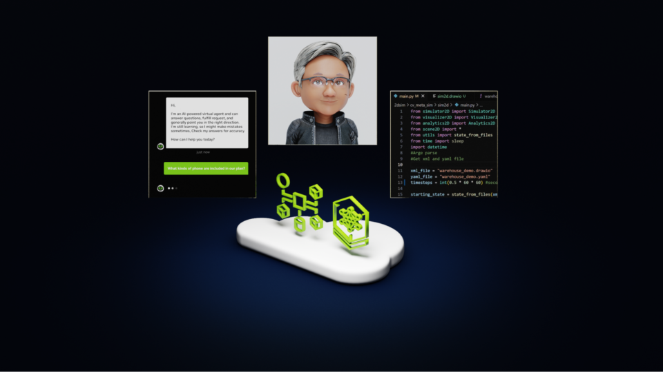
The rise of test-time compute unlocks the ability for AI to offer well-reasoned, helpful and more accurate responses to complex, open-ended user queries. These capabilities will be critical for the detailed, multistep reasoning tasks expected of autonomous agentic AI and physical AI applications. Across industries, they could boost efficiency and productivity by providing users with highly capable assistants to accelerate their work.
In healthcare, models could use test-time scaling to analyze vast amounts of data and infer how a disease will progress, as well as predict potential complications that could stem from new treatments based on the chemical structure of a drug molecule. Or, it could comb through a database of clinical trials to suggest options that match an individual’s disease profile, sharing its reasoning process about the pros and cons of different studies.
In retail and supply chain logistics, long thinking can help with the complex decision-making required to address near-term operational challenges and long-term strategic goals. Reasoning techniques can help businesses reduce risk and address scalability challenges by predicting and evaluating multiple scenarios simultaneously — which could enable more accurate demand forecasting, streamlined supply chain travel routes, and sourcing decisions that align with an organization’s sustainability initiatives.
And for global enterprises, this technique could be applied to draft detailed business plans, generate complex code to debug software, or optimize travel routes for delivery trucks, warehouse robots and robotaxis.
AI reasoning models are rapidly evolving. OpenAI o1-mini and o3-mini, DeepSeek R1, and Google DeepMind’s Gemini 2.0 Flash Thinking were all introduced in the last few weeks, and additional new models are expected to follow soon.
Models like these require considerably more compute to reason during inference and generate correct answers to complex questions — which means that enterprises need to scale their accelerated computing resources to deliver the next generation of AI reasoning tools that can support complex problem-solving, coding and multistep planning.
Learn about the benefits of NVIDIA AI for accelerated inference.

The rapid evolution of generative AI has created countless opportunities for innovation across industry and research. As is often the case with state-of-the-art technology, this evolution has also shifted the landscape of cybersecurity threats, creating new security requirements. Critical infrastructure cybersecurity is advancing to thwart the next wave of emerging threats in the AI era.
Leading operational technology (OT) providers today showcased at the S4 conference for industrial control systems (ICS) and OT cybersecurity how they’re adopting the NVIDIA cybersecurity AI platform to deliver real-time threat detection and critical infrastructure protection.
Armis, Check Point, CrowdStrike, Deloitte and World Wide Technology (WWT) are integrating the platform to help customers bolster critical infrastructure, such as energy, utilities and manufacturing facilities, against cyber threats.
Critical infrastructure operates in highly complex environments, where the convergence of IT and OT, often accelerated by digital transformation, creates a perfect storm of vulnerabilities. Traditional cybersecurity measures are no longer sufficient to address these emerging threats.
By harnessing NVIDIA’s cybersecurity AI platform, these partners can provide exceptional visibility into critical infrastructure environments, achieving robust and adaptive security while delivering operational continuity.
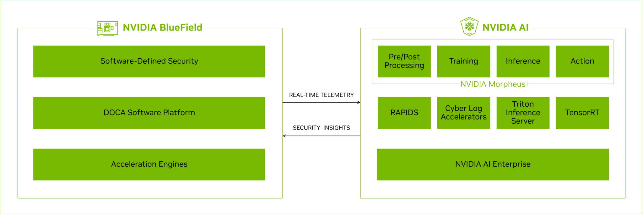
The platform integrates NVIDIA’s accelerated computing and AI, featuring NVIDIA BlueField-3 DPUs, NVIDIA DOCA and the NVIDIA Morpheus AI cybersecurity framework, part of the NVIDIA AI Enterprise. This combination enables real-time threat detection, empowering cybersecurity professionals to respond swiftly at the edge and across networks.
Unlike conventional solutions that depend on intrusive methods or software agents, BlueField-3 DPUs function as a virtual security overlay. They inspect network traffic and safeguard host integrity without disrupting operations. Acting as embedded sensors within each server, they stream telemetry data to NVIDIA Morpheus, enabling detailed monitoring of host activities, network traffic and application behaviors — seamlessly and without operational impact.
Integrating Armis Centrix, Armis’ AI-powered cyber exposure management platform, with NVIDIA cybersecurity AI helps secure critical infrastructure like energy, manufacturing, healthcare and transportation.
“OT environments are increasingly targeted by sophisticated cyber threats, requiring robust solutions that ensure both security and operational continuity,” said Nadir Izrael, chief technology officer and cofounder of Armis. “Combining Armis’ unmatched platform for OT security and cyber exposure management with NVIDIA BlueField-3 DPUs enables organizations to comprehensively protect cyber-physical systems without disrupting operations.”
CrowdStrike is helping secure critical infrastructure such as ICS and OT by deploying its CrowdStrike Falcon security agent on BlueField-3 DPUs to boost real-time AI-powered threat detection and response.
“OT environments are under increasing threat, demanding AI-powered security that adapts in real time,” said Raj Rajamani, head of products at CrowdStrike. “By integrating NVIDIA BlueField-3 DPUs with the CrowdStrike Falcon platform, we’re extending industry-leading protection to critical infrastructure without disrupting operations — delivering unified protection at the edge and helping organizations stay ahead of modern threats.”
Deloitte is driving customers’ digital transformation, enabled by NVIDIA’s cybersecurity AI platform, to help meet the demands of breakthrough technologies that require real-time, granular visibility into data center networks to defend against increasingly sophisticated threats.
“Protecting OT and ICS systems is becoming increasingly challenging as organizations embrace digital transformation and interconnected technologies,” said Dmitry Dudorov, an AI security leader at Deloitte U.K. “Harnessing NVIDIA’s cybersecurity AI platform can enable organizations to determine threat detection, enhance resilience and safeguard their infrastructure to accelerate their efforts.”
NVIDIA’s cybersecurity AI platform, combined with the expertise of ecosystem partners, offers a powerful and scalable solution to protect critical infrastructure environments against evolving threats. Bringing NVIDIA AI and accelerated computing to the forefront of OT security can help organizations protect what matters most — now and in the future.
Learn more by attending the NVIDIA GTC global AI conference, running March 17-21, where Armis, Check Point and CrowdStrike cybersecurity leaders will host sessions about their collaborations with NVIDIA.

 Google and Institut Curie are embarking on a journey together to revolutionize the fight against women’s cancers.Read More
We’re excited to have PyTorch sponsor Datathon 2025: DataOrbit, a place where students can collaborate with a team to solve problems using real-world datasets! This event, hosted by Data Science UCSB in collaboration with Gaucho Sports Analytics and ACM@UCSB, will take place on February 22–23rd, 2025 at UC Santa Barbara, with the incredible opportunity to present your project to a panel of corporate and faculty judges – including the executive director of Pytorch! – for a chance to win prizes up to $3000.

PyTorch’s versatility and power have made it an essential tool for tackling complex data problems in domains ranging from computer vision and natural language processing to time series analysis. At Datathon 2025: DataOrbit, participants will have the chance to leverage PyTorch’s dynamic framework, ease of use, and robust ecosystem to build innovative solutions. Whether you’re building machine learning models, experimenting with deep learning architectures, or applying PyTorch to solve real-world challenges, workshops and mentors will be available to help you dive deeper into its capabilities and accelerate your project’s success.
Register Here: tinyurl.com/dataorbit25-reg (Open until February 21st or until capacity is reached)
Additional information regarding the timeline of events can be found on the registration form.
About the Datathon
If you have a group you would like to work with, we require that every member register separately. If you do not have a group, we will have an opportunity at the beginning of the event to participate in an activity to form groups. Unfortunately, at this time we do not provide travel accommodations or lodging for participants.
If you are interested in mentoring students virtually during the course of our datathon, or have any other questions contact us at datascience.ucsb@gmail.com.


