Today, we’re excited to announce the availability of Llama 4 Scout and Maverick models in Amazon SageMaker JumpStart and coming soon in Amazon Bedrock. Llama 4 represents Meta’s most advanced multimodal models to date, featuring a mixture of experts (MoE) architecture and context window support up to 10 million tokens. With native multimodality and early fusion technology, Meta states that these new models demonstrate unprecedented performance across text and vision tasks while maintaining efficient compute requirements. With a dramatic increase on supported context length from 128K in Llama 3, Llama 4 is now suitable for multi-document summarization, parsing extensive user activity for personalized tasks, and reasoning over extensive codebases. You can now deploy the Llama-4-Scout-17B-16E-Instruct, Llama-4-Maverick-17B-128E-Instruct, and Llama-4-Maverick-17B-128E-Instruct-FP8 models using SageMaker JumpStart in the US East (N. Virginia) AWS Region.

In this blog post, we walk you through how to deploy and prompt a Llama-4-Scout-17B-16E-Instruct model using SageMaker JumpStart.

Llama 4 overview

Meta announced Llama 4 today, introducing three distinct model variants: Scout, which offers advanced multimodal capabilities and a 10M token context window; Maverick, a cost-effective solution with a 128K context window; and Behemoth, in preview. These models are optimized for multimodal reasoning, multilingual tasks, coding, tool-calling, and powering agentic systems.

Llama 4 Maverick is a powerful general-purpose model with 17 billion active parameters, 128 experts, and 400 billion total parameters, and optimized for high-quality general assistant and chat use cases. Additionally, Llama 4 Maverick is available with base and instruct models in both a quantized version (FP8) for efficient deployment on the Instruct model and a non-quantized (BF16) version for maximum accuracy.

Llama 4 Scout, the more compact and smaller model, has 17 billion active parameters, 16 experts, and 109 billion total parameters, and features an industry-leading 10M token context window. These models are designed for industry-leading performance in image and text understanding with support for 12 languages, enabling the creation of AI applications that bridge language barriers.

See Meta’s community license agreement for usage terms and more details.

SageMaker JumpStart overview

SageMaker JumpStart offers access to a broad selection of publicly available foundation models (FMs). These pre-trained models serve as powerful starting points that can be deeply customized to address specific use cases. You can use state-of-the-art model architectures—such as language models, computer vision models, and more—without having to build them from scratch.

With SageMaker JumpStart, you can deploy models in a secure environment. The models can be provisioned on dedicated SageMaker inference instances can be isolated within your virtual private cloud (VPC). After deploying an FM, you can further customize and fine-tune it using the extensive capabilities of Amazon SageMaker AI, including SageMaker inference for deploying models and container logs for improved observability. With SageMaker AI, you can streamline the entire model deployment process.

Prerequisites

To try the Llama 4 models in SageMaker JumpStart, you need the following prerequisites:

• An AWS account that will contain all your AWS resources.
• An AWS Identity and Access Management (IAM) role to access SageMaker AI. To learn more about how IAM works with SageMaker AI, see Identity and Access Management for Amazon SageMaker AI.
• Access to Amazon SageMaker Studio and a SageMaker AI notebook instance or an interactive development environment (IDE) such as PyCharm or Visual Studio Code. We recommend using SageMaker Studio for straightforward deployment and inference.
• Access to accelerated instances (GPUs) for hosting the LLMs.

Discover Llama 4 models in SageMaker JumpStart

SageMaker JumpStart provides FMs through two primary interfaces: SageMaker Studio and the Amazon SageMaker Python SDK. This provides multiple options to discover and use hundreds of models for your specific use case.

SageMaker Studio is a comprehensive integrated development environment (IDE) that offers a unified, web-based interface for performing all aspects of the AI development lifecycle. From preparing data to building, training, and deploying models, SageMaker Studio provides purpose-built tools to streamline the entire process.

In SageMaker Studio, you can access SageMaker JumpStart to discover and explore the extensive catalog of FMs available for deployment to inference capabilities on SageMaker Inference. You can access SageMaker JumpStart by choosing JumpStart in the navigation pane or by choosing JumpStart from the Home page in SageMaker Studio, as shown in the following figure.

Alternatively, you can use the SageMaker Python SDK to programmatically access and use SageMaker JumpStart models. This approach allows for greater flexibility and integration with existing AI and machine learning (AI/ML) workflows and pipelines.

By providing multiple access points, SageMaker JumpStart helps you seamlessly incorporate pre-trained models into your AI/ML development efforts, regardless of your preferred interface or workflow.

Deploy Llama 4 models for inference through the SageMaker JumpStart UI

On the SageMaker JumpStart landing page, you can find all the public pre-trained models offered by SageMaker AI. You can then choose the Meta model provider tab to discover all the available Meta models.

If you’re using SageMaker Classic Studio and don’t see the Llama 4 models, update your SageMaker Studio version by shutting down and restarting. For more information about version updates, see Shut down and Update Studio Classic Apps.

1. Search for Meta to view the Meta model card. Each model card shows key information, including:
   • Model name
   • Provider name
   • Task category (for example, Text Generation)
2. Select the model card to view the model details page.
   

The model details page includes the following information:

• The model name and provider information
• Deploy button to deploy the model
• About and Notebooks tabs with detailed information

The About tab includes important details, such as:

• Model description
• License information
• Technical specifications
• Usage guidelines

Before you deploy the model, we recommended you review the model details and license terms to confirm compatibility with your use case.

3. Choose Deploy to proceed with deployment.
   

4. For Endpoint name, use the automatically generated name or enter a custom one.
5. For Instance type, use the default: p5.48xlarge.
6. For Initial instance count, enter the number of instances (default: 1).
   Selecting appropriate instance types and counts is crucial for cost and performance optimization. Monitor your deployment to adjust these settings as needed.
7. Under Inference type, Real-time inference is selected by default. This is optimized for sustained traffic and low latency.
8. Review all configurations for accuracy. For this model, we strongly recommend adhering to SageMaker JumpStart default settings and making sure that network isolation remains in place.
9. Choose Deploy. The deployment process can take several minutes to complete.
   

When deployment is complete, your endpoint status will change to InService. At this point, the model is ready to accept inference requests through the endpoint. You can monitor the deployment progress on the SageMaker console Endpoints page, which will display relevant metrics and status information. When the deployment is complete, you can invoke the model using a SageMaker runtime client and integrate it with your applications.

Deploy Llama 4 models for inference using the SageMaker Python SDK

When you choose Deploy and accept the terms, model deployment will start. Alternatively, you can deploy through the example notebook by choosing Open Notebook. The notebook provides end-to-end guidance on how to deploy the model for inference and clean up resources.

To deploy using a notebook, start by selecting an appropriate model, specified by the model_id. You can deploy any of the selected models on SageMaker AI.

You can deploy the Llama 4 Scout model using SageMaker JumpStart with the following SageMaker Python SDK code:

from sagemaker.jumpstart.model import JumpStartModel

model = JumpStartModel(model_id = "meta-vlm-llama-4-scout-17b-16e-instruct")

predictor = model.deploy(accept_eula=False)

This deploys the model on SageMaker AI with default configurations, including default instance type and default VPC configurations. You can change these configurations by specifying non-default values in JumpStartModel. To successfully deploy the model, you must manually set accept_eula=True as a deploy method argument. After it’s deployed, you can run inference against the deployed endpoint through the SageMaker predictor:

payload = {
"messages": [
 {"role": "system", "content": "You are a helpful assistant"},
 {"role": "user", "content": "How are you doing today"},
 {"role": "assistant", "content": "Good, what can i help you with today?"},
 {"role": "user", "content": "Give me 5 steps to become better at tennis?"}
],
 "temperature": 0.6,
 "top_p": 0.9,
 "max_tokens": 512,
 "logprobs": False
} 
response = predictor.predict(payload) 
response_message = response['choices'][0]['message']['content']

Recommended instances and benchmark

The following table lists all the Llama 4 models available in SageMaker JumpStart along with the model_id, default instance types, and the maximum number of total tokens (sum of number of input tokens and number of generated tokens) supported for each of these models. For increased context length, you can modify the default instance type in the SageMaker JumpStart UI.

Inference and example prompts for Llama 4 Scout 17B 16 Experts model

You can use the Llama 4 Scout model for text and image or vision reasoning use cases. With that model, you can perform a variety of tasks, such as image captioning, image text retrieval, visual question answering and reasoning, document visual question answering, and more.

In the following sections we show example payloads, invocations, and responses for Llama 4 Scout that you can use against your Llama 4 model deployments using Sagemaker JumpStart.

Text-only input

Input:

payload = {
    "messages": [
        {
            "role": "system",
            "content": "You are a helpful AI assistant."
        },
        {
            "role": "user",
            "content": "What are three key benefits of large language models for businesses?"
        }
    ],
    "max_tokens": 2048,
    "temperature": 0.7,
    "top_p": 0.9,
    "stream": False
}

Response:

Large language models (LLMs) offer numerous benefits to businesses, transforming how they operate, 
interact with customers, and generate insights. Here are three key benefits:

1. **Enhanced Customer Experience through Automation and Personalization**:
   - **Automated Customer Support**: LLMs can power chatbots and virtual assistants 
	that provide 24/7 customer support. These models can understand and respond to a wide range of customer queries, help with troubleshooting, and even process transactions, significantly reducing the workload on human customer support agents.
   - **Personalization**: By analyzing customer data, LLMs can help businesses personalize their 
	communications and offerings. For instance, they can generate personalized emails, product recommendations, and content, enhancing customer engagement and satisfaction.

2. **Efficiency and Productivity Gains**:
   - **Content Generation**: LLMs can automate the creation of various types of content, such as 
   blog posts, reports, product descriptions, and social media updates. This not only speeds up content production but also allows human writers to focus on more creative and strategic tasks.
   - **Data Analysis and Summarization**: These models can quickly analyze large volumes of data, extract relevant information, and summarize findings in a readable format. This capability can significantly reduce the time and effort required for market research, competitive analysis, and internal reporting.

3. **Improved Decision Making with Data-Driven Insights**:
   - **Market and Trend Analysis**: LLMs can process and analyze vast amounts of data from various sources, including news articles, social media, and market reports. This helps businesses stay informed about market trends, consumer sentiment, and competitor activity, enabling more informed strategic decisions.
   - **Risk Management and Compliance**: By analyzing regulatory documents and monitoring communications, LLMs can help businesses identify and mitigate compliance risks. They can also assist in the creation of compliance reports and documentation, reducing the risk of human error.

In summary, large language models offer businesses the potential to automate and enhance customer interactions, 
improve operational efficiency, and gain deeper insights from their data. These capabilities can lead to cost savings, 
increased revenue, and a competitive edge in the market.

Single-image input

In this section, let’s test Llama 4’s multimodal capabilities. By merging text and vision tokens into a unified processing backbone, Llama 4 can seamlessly understand and respond to queries about an image. The following is an example of how you can prompt Llama 4 to answer questions about an image such as the one in the example:

Image:

Input:

import requests
import base64
import boto3
import json

s3 = boto3.client("s3")

s3_bucket = f"jumpstart-cache-prod-{region}"
key_prefix = "inference-notebook-assets"

def download_from_s3(key_filenames):
    for key_filename in key_filenames:
        s3.download_file(s3_bucket, f"{key_prefix}/{key_filename}", key_filename)

# Define image names
heat_map = "heatmap_semantic_similarity_search.png"

# Download and display the heatmap image
download_from_s3(key_filenames=[heat_map])

def img_to_base64(image_path):
    with open(image_path, "rb") as f:
        img = f.read()
    enc_img = base64.b64encode(img).decode('utf-8')
    return enc_img

b64_img = img_to_base64(heat_map)

data = {
    "messages": [
        {
            "role": "system",
            "content": "You are a helpful assistant",
        },
        {
            "role": "user",
            "content": [
                {
                    "type": "text",
                    "text": "What is in this image?",
                },
                {
                    "type": "image_url",
                    "image_url": {
                        "url": b64_img
                    }
                },
            ],
        },
    ],
    "temperature": 0.6,
    "top_p": 0.9,
    "max_tokens": 512
}

payload = json.dumps(data)

Response:

The image presents a heatmap illustrating the semantic textual similarity between 
sentences. The heatmap is divided into two axes, with the x-axis listing six sentences 
and the y-axis listing the same six sentences in a different order.nn**Sentences:**nn* 
Your dog is so cute.n* How cute your dog is!n* You have such a cute dog!n* New York City 
is the place where I work.n* I work in New York City.n* What color do you like the most?n* 
What is your favourite color?nn**Heatmap:**nnThe heatmap displays the semantic textual 
similarity between each pair of sentences, with darker shades of red indicating higher similarity 
and lighter shades of orange indicating lower similarity. The color bar on the right side of the 
heatmap provides a scale for interpreting the similarity values, ranging from -0.4 to 1.0.nn
**Observations:**nn* The three sentences related to dogs ("Your dog is so cute.", "How cute your dog is!", 
and "You have such a cute dog!") show high similarity with each other, as indicated by the dark red squares 
in the corresponding section of the heatmap.n* The two sentences related to New York City ("New York City is 
the place where I work." and "I work in New York City.") also show high similarity with each other.n* The two 
sentences related to favorite colors ("What color do you like the most?" and "What is your favorite color?") 
show high similarity with each other.n* The sentences from different categories (dogs, New York City, and 
favorite colors) show lower similarity with each other, as indicated by the lighter shades of orange in the heatmap.nn
Overall, the heatmap effectively visualizes the semantic textual similarity between the given sentences, allowing 
for easy identification of similar and dissimilar sentence pairs.

The Llama 4 model on JumpStart can take in the image provided via a URL, underlining its powerful potential for real-time multimodal applications.

Multi-image input

Building on its advanced multimodal functionality, Llama 4 can effortlessly process multiple images at the same time. In this demonstration, the model is prompted with two image URLs and tasked with describing each image and explaining their relationship, showcasing its capacity to synthesize information across several visual inputs. Let’s test this below by passing in the URLs of the following images in the payload.

Image 1:

Image 2:

Input: 

def url_to_base64(image_url):
    # Download the image
    response = requests.get(image_url)
    if response.status_code != 200:
        return None

    # Encode the image content to base64
    image_base64 = base64.b64encode(response.content).decode('utf-8')
    return image_base64

image_url_2 = "https://raw.githubusercontent.com/mathvision-cuhk/MATH-V/refs/heads/main/images/13.jpg"
b64_img_url_2 = url_to_base64(image_url_2)

data = {
    "messages": [
        {
            "role": "system",
            "content": "You are a helpful assistant",
        },
        {
            "role": "user",
            "content": [
                {
                    "type": "text",
                    "text": "There are two images. Describe each one and why they are related",
                },
                {
                    "type": "image_url",
                    "image_url": {
                        "url": b64_img,
                    }
                },
                {
                    "type": "image_url",
                    "image_url": {
                        "url": b64_img_url_2,
                    }
                },
            ],
        },
    ],
    "temperature": 0.6,
    "top_p": 0.9,
    "max_tokens": 512
}

Response:

The first image is a heatmap illustrating the semantic textual similarity between 
sentences. The heatmap is titled "Semantic Textual Similarity Between Sentences" 
and features a color scale ranging from -0.4 to 1.0, with darker shades indicating 
higher similarity. The sentences being compared are:nn* Your dog is so cute.n* 
How cute your dog is!n* You have such a cute dog!n* New York City is the place 
where I work.n* I work in New York City.n* What color do you like the most?n* 
What is your favourite color?nnThe heatmap reveals that the sentences about dogs 
have high similarity scores, with values above 0.9, indicating that they convey 
similar meanings. Similarly, the sentences about work locations and favorite colors 
also show high similarity scores. However, there is a low similarity score between 
the sentences about dogs and those about work locations or favorite colors.nn
The second image presents five stick figures labeled A, B, C, D, and E, each representing
a person. The figures are drawn using simple lines and geometric shapes, such as circles
for heads, squares for bodies, and triangles for skirts. The main difference between the
figures lies in their arm and leg positions:nn* Figure A has its arms at its sides and 
straight legs.n* Figure B has its arms at its sides and straight legs, but with a slightly 
different posture.n* Figure C has its arms at its sides and straight legs, similar to Figure A.n*
Figure D has one arm raised and straight legs.n* Figure E has two arms raised and bent legs.nn
Overall, the two images are distinct in terms of their content and purpose. The heatmap provides a 
visual representation of semantic similarities between sentences, while the stick figures appear to 
be simple illustrations of people with varying poses.

As you can see, Llama 4 excels in handling multiple images simultaneously, providing detailed and contextually relevant insights that emphasize its robust multimodal processing abilities.

Codebase analysis with Llama 4

Using Llama 4 Scout’s industry-leading context window, this section showcases its ability to deeply analyze expansive codebases. The example extracts and contextualizes the buildspec-1-10-2.yml file from the AWS Deep Learning Containers GitHub repository, illustrating how the model synthesizes information across an entire repository. We used a tool to ingest the whole repository into plaintext that we provided to the model as context:

Input:

payload = {
    "messages": [
        {
            "role": "system",
            "content": """You are a helpful AI assistant that summarizes codebases to me to help me understand
            how to analyze code by synthesizing through the entire codebase before responding.
            
            Be thorough in your search as the file may be nested within a markdown code block or within a directory listing.
            """
        },
        {
            "role": "user",
            "content": f"Can you explain to me the buildspec-1-10-2.yml file and how it relates to the rest of the huggingface directory? Here is the AWS Deep Learning Container Repository for reference:nn{text}"
        }
    ],
    "max_tokens": 2048,
    "temperature": 0.7,
    "top_p": 0.9,
    "stream": False
}

Output: 

## Overview of the buildspec-1-10-2.yml File

The provided information appears to be a part of a large, merged representation of 
the Hugging Face repository, generated by Repomix. The `buildspec-1-10-2.yml` file 
is likely a build specification file used in a Continuous Integration/Continuous 
Deployment (CI/CD) pipeline.

## Purpose and Format

The file contains a packed representation of the entire repository's contents, designed
 to be easily consumable by AI systems for analysis, code review, or other automated processes. 
The content is organized into sections:

1.  **Summary**: Provides an overview of the file's purpose, format, and usage guidelines.
2.  **Repository Information**: Not shown in the provided excerpt, but likely contains metadata about the repository.
3.  **Directory Structure**: Lists the directory structure of the repository, including file paths.
4.  **File Entries**: Each file entry consists of a header with the file path and the full contents 
of the file in a code block.

## Relationship to the Hugging Face Directory

The `buildspec-1-10-2.yml` file is part of the Hugging Face repository, which appears to be a 
large project with multiple subdirectories and files. The directory structure section lists various 
subdirectories, including:

*   `.github/`: Contains GitHub-related configuration files, such as issue templates, workflows, 
and CODEOWNERS.
*   `.release_templates/`: Includes release image templates for various frameworks like MXNet, PyTorch, 
and TensorFlow.
*   `autogluon/`: A subdirectory with build artifacts, inference configurations, and other related files.

## buildspec-1-10-2.yml File Contents

Unfortunately, the provided excerpt does not contain the actual contents of the `buildspec-1-10-2.yml` file. 
However, based on the file name and its presence in a CI/CD context, it is likely that this file specifies 
the build process, dependencies, and environment configurations for the Hugging Face project.

## Usage Guidelines

When working with this file, keep in mind:

*   Treat this file as read-only and make changes to the original repository files instead.
*   Use the file path to distinguish between different files in the repository.
*   Handle this file with the same level of security as the original repository, as it may 
contain sensitive information.

## Additional Notes

*   Some files might be excluded based on `.gitignore` rules and Repomix's configuration.
*   Binary files are not included in this packed representation.
*   Files are sorted by Git change count, with files having more changes appearing at the bottom.

## Example Use Case

To analyze the `buildspec-1-10-2.yml` file, you would:

1.  Locate the file in the repository directory structure.
2.  Review the file contents to understand the build process, dependencies, and environment configurations.
3.  Use this information to optimize the build process, troubleshoot issues, or make changes to the repository.

Keep in mind that the actual contents of the `buildspec-1-10-2.yml` file are not provided, so this 
is a general explanation based on the file name and context. 

To get the actual content you would look for 

## File: buildspec-1-10-2.yml 

 block and read its content 

Let me know if I can assist with anything else.

Multi-document processing

Harnessing the same extensive token context window, Llama 4 Scout excels in multi-document processing. In this example, the model extracts key financial metrics from Amazon 10-K reports (2017-2024), demonstrating its capability to integrate and analyze data spanning multiple years—all without the need for additional processing tools.

Input: 

payload = {
    "messages": [
        {
            "role": "system",
            "content": "You are a financial analyst. Extract key financial data from this 10-K report."
        },
        {
            "role": "user",
            "content": f"""Extract the following information from this Amazon 10-K report:
            1. What year is this report for?
            2. Total revenue for the year
            3. Net income
            4. Key business segments and their performance
            5. Important trends mentioned
            
            Here's the 10-K text:
            {pdf_text[:25000]}
            
            Format your response as a JSON object with these fields: year, revenue, net_income, segments, trends.
            """
        }
    ],
    "max_tokens": 2048,
    "temperature": 0.7,
    "top_p": 0.9,
    "stream": False
}

Output:

To analyze Amazon's growth from 2017 to 2024, we'll examine the revenue and net income 
data available from the 10-K reports.

### Revenue Growth

| Year | Revenue (in billion USD) |
| --- | --- |
| 2014 | 89 |
| 2015 | 107 |
| 2016 | 135.99 |
| 2017 | 177.87 |
| 2018 | 232.88 |
| 2019 | 280.52 |
| 2020 | 386.06 |
| 2021 | 478 |
| 2022 | 513 |
| 2023 | 513.98 |
| 2024 | 574.78 (projected) |

From 2017 to 2024, Amazon's revenue has grown from $177.87 billion to a projected $574.78 billion, 
representing a significant increase of approximately 223% over the 7-year period.

### Net Income Growth

| Year | Net Income (in billion USD) |
| --- | --- |
| 2014 | 0.236 |
| 2015 | 0.596 |
| 2016 | 2.37 |
| 2017 | 3.03 |
| 2018 | 10.07 |
| 2019 | 11.59 |
| 2020 | 18.68 |
| 2021 | 33.4 |
| 2022 | 18.7 (lower due to economic conditions) |
| 2023 | 33.36 |
| 2024 | 37.68 (projected) |

Amazon's net income has grown from $3.03 billion in 2017 to a projected $37.68 billion in 2024, 
representing a substantial increase of approximately 1143% over the 7-year period.

### Segment and Trend Analysis

Throughout the years, Amazon has maintained its three main business segments: North America, 
International, and Amazon Web Services (AWS). The company has continued to expand into new products, 
services, technologies, and geographic regions, driving growth and increasing competition.

The trends mentioned across the 10-K reports highlight the company's:

1. **Seasonality**: Higher sales volume during the fourth quarter.
2. **Intense competition**: Across geographies and industries, including e-commerce, cloud computing, 
and digital content.
3. **Expansion**: Into new products, services, technologies, and geographic regions, which subjects 
the company to additional business, legal, financial, and competitive risks.
4. **International operations**: Subject to risks such as local economic and political conditions, 
government regulation, and restrictions on sales or distribution.

### Conclusion

Amazon has demonstrated remarkable growth from 2017 to 2024, with revenue increasing by 
approximately 223% and net income growing by approximately 1143%. The company's continued 
expansion into new areas, its strong presence in cloud computing through AWS, and its ability 
to adapt to changing market conditions have contributed to its success. However, the company 
also faces intense competition, seasonality, and risks associated with international operations.

--------------------------------------------------
Ask a question about the Amazon 10-K reports across years.

Clean up

To avoid incurring unnecessary costs, when you’re done, delete the SageMaker endpoints using the following code snippets:

predictor.delete_model()
predictor.delete_endpoint()

Alternatively, using the SageMaker console, complete the following steps:

1. On the SageMaker console, under Inference in the navigation pane, choose Endpoints.
2. Search for the embedding and text generation endpoints.
3. On the endpoint details page, choose Delete.
4. Choose Delete again to confirm.

Conclusion

In this post, we explored how SageMaker JumpStart empowers data scientists and ML engineers to discover, access, and deploy a wide range of pre-trained FMs for inference, including Meta’s most advanced and capable models to date. Get started with SageMaker JumpStart and Llama 4 models today.

For more information about SageMaker JumpStart, see Train, deploy, and evaluate pretrained models with SageMaker JumpStart and Getting started with Amazon SageMaker JumpStart.

About the authors

Marco Punio is a Sr. Specialist Solutions Architect focused on generative AI strategy, applied AI solutions, and conducting research to help customers hyper-scale on AWS. As a member of the Third-party Model Provider Applied Sciences Solutions Architecture team at AWS, he is a global lead for the Meta–AWS Partnership and technical strategy. Based in Seattle, Washington, Marco enjoys writing, reading, exercising, and building applications in his free time.

Chakravarthy Nagarajan is a Principal Solutions Architect specializing in machine learning, big data, and high performance computing. In his current role, he helps customers solve real-world, complex business problems using machine learning and generative AI solutions.

Banu Nagasundaram leads product, engineering, and strategic partnerships for Amazon SageMaker JumpStart, the SageMaker machine learning and generative AI hub. She is passionate about building solutions that help customers accelerate their AI journey and unlock business value.

Malav Shastri is a Software Development Engineer at AWS, where he works on the Amazon SageMaker JumpStart and Amazon Bedrock teams. His role focuses on enabling customers to take advantage of state-of-the-art open source and proprietary foundation models and traditional machine learning algorithms. Malav holds a Master’s degree in Computer Science.

Niithiyn Vijeaswaran is a Generative AI Specialist Solutions Architect with the Third-party Model Science team at AWS. His area of focus is AWS AI accelerators (AWS Neuron). He holds a Bachelor’s degree in Computer Science and Bioinformatics.

Baladithya Balamurugan is a Solutions Architect at AWS focused on ML deployments for inference and using AWS Neuron to accelerate training and inference. He works with customers to enable and accelerate their ML deployments on services such as Amazon Sagemaker and Amazon EC2. Based in San Francisco, Baladithya enjoys tinkering, developing applications, and his home lab in his free time.

John Liu has 14 years of experience as a product executive and 10 years of experience as a portfolio manager. At AWS, John is a Principal Product Manager for Amazon Bedrock. Previously, he was the Head of Product for AWS Web3 and Blockchain. Prior to AWS, John held various product leadership roles at public blockchain protocols and fintech companies, and also spent 9 years as a portfolio manager at various hedge funds.

Read More

Amazon Bedrock is a fully managed service that offers a choice of high-performing foundation models (FMs) from leading AI companies and AWS. Amazon Bedrock Knowledge Bases offers fully managed, end-to-end Retrieval Augmented Generation (RAG) workflows to create highly accurate, low-latency, secure, and custom generative AI applications by incorporating contextual information from your company’s data sources.

Organizations need to control access to their data across different business units, including companies, departments, or even individuals, while maintaining scalability. When organizations try to separate data sources manually, they often create unnecessary complexity and hit service limitations. This post demonstrates how Amazon Bedrock Knowledge Bases can help you scale your data management effectively while maintaining proper access controls on different management levels.

One of these strategies is using Amazon Simple Storage Service (Amazon S3) folder structures and Amazon Bedrock Knowledge Bases metadata filtering to enable efficient data segmentation within a single knowledge base. Additionally, we dive into integrating common vector database solutions available for Amazon Bedrock Knowledge Bases and how these integrations enable advanced metadata filtering and querying capabilities.

Organizing S3 folder structures for scalable knowledge bases

Organizations working with multiple customers need a secure and scalable way to keep each customer’s data separate while maintaining efficient access controls. Without proper data segregation, companies risk exposing sensitive information between customers or creating complex, hard-to-maintain systems. For this post, we focus on maintaining access controls across multiple business units within the same management level.

A key strategy involves using S3 folder structures and Amazon Bedrock Knowledge Bases metadata filtering to enable efficient data segregation within a single knowledge base. Instead of creating separate knowledge bases for each customer, you can use a consolidated knowledge base with a well-structured S3 folder hierarchy. For example, imagine a consulting firm that manages documentation for multiple healthcare providers—each customer’s sensitive patient records and operational documents must remain strictly separated. The Amazon S3 structure might look as follows:

s3://amzn-s3-demo-my-knowledge-base-bucket/customer-data/

    s3://amzn-s3-demo-my-knowledge-base-bucket/customer-data/customerA/

        s3://amzn-s3-demo-my-knowledge-base-bucket/customer-data/customerA/policies/

        s3://amzn-s3-demo-my-knowledge-base-bucket/customer-data/customerA/procedures/

    s3://amzn-s3-demo-my-knowledge-base-bucket/customer-data/customerB/

        s3://amzn-s3-demo-my-knowledge-base-bucket/customer-data/customerB/policies/

        s3://amzn-s3-demo-my-knowledge-base-bucket/customer-data/customerB/procedures/

This structure makes sure that Customer A’s healthcare documentation remains completely separate from Customer B’s data. When combined with Amazon Bedrock Knowledge Bases metadata filtering, you can verify that users associated with Customer A can only access their organization’s documents, and Customer B’s users can only see their own data—maintaining strict data boundaries while using a single, efficient knowledge base infrastructure.

The Amazon Bedrock Knowledge Bases metadata filtering capability enhances this segregation by allowing you to tag documents with customer-specific identifiers and other relevant attributes. These metadata filters provide an additional layer of security and organization, making sure that queries only return results from the appropriate customer’s dataset.

Solution overview

The following diagram provides a high-level overview of AWS services and features through a sample use case. Although the example uses Customer A and Customer B for illustration, these can represent distinct business units (such as departments, companies, or teams) with different compliance requirements, rather than only individual customers.

The workflow consists of the following steps:

1. Customer data is uploaded along with metadata indicating data ownership and other properties to specific folders in an S3 bucket.
2. The S3 bucket, containing customer data and metadata, is configured as a knowledge base data source. Amazon Bedrock Knowledge Bases ingests the data, along with the metadata, from the source repository and a knowledge base sync is performed.
3. A customer initiates a query using a frontend application with metadata filters against the Amazon Bedrock knowledge base. An access control metadata filter must be in place to make sure that the customer only accesses data they own; the customer can apply additional filters to further refine query results. This combined query and filter is passed to the RetrieveAndGenerate API.
4. The RetrieveAndGenerate API handles the core RAG workflow. It consists of several sub-steps:
   • The user query is converted into a vector representation (embedding).
   • Using the query embedding and the metadata filter, relevant documents are retrieved from the knowledge base.
   • The original query is augmented with the retrieved documents, providing context for the large language model (LLM).
   • The LLM generates a response based on the augmented query and retrieved context.
5. Finally, the generated response is sent back to the user.

When implementing Amazon Bedrock Knowledge Bases in scenarios involving sensitive information or requiring access controls, developers must implement proper metadata filtering in their application code. Failure to enforce appropriate metadata-based filtering could result in unauthorized access to sensitive documents within the knowledge base. Metadata filtering serves as a critical security boundary and should be consistently applied across all queries. For comprehensive guidance on implementing secure metadata filtering practices, refer to the Amazon Bedrock Knowledge Base Security documentation.

Implement metadata filtering

For this use case, two specific example customers, Customer A and Customer B, are aligned to different proprietary compliance documents. The number of customers and folders can scale to N depending on the size of the customer base. We will use the following public documents, which will reside in the respective customer’s S3 folder. Customer A requires the Architecting for HIPAA Security and Compliance on AWS document. Customer B requires access to the  Using AWS in the Context of NHS Cloud Security Guidance  document.

1. Create a JSON file representing the corresponding metadata for both Customer A and Customer B:

The following is the JSON metadata for Customer A’s data:

{ "metadataAttributes": { "customer": "CustomerA", "documentType": "HIPAA Compliance Guide", "focus": "HIPAA Compliance", "publicationYear": 2022, "region": "North America" }}

The following is the JSON metadata for Customer B’s data:

{ "metadataAttributes": { "customer": "CustomerB", "documentType": "NHS Compliance Guidance", "focus": "UK Healthcare Compliance", "publicationYear": 2023, "region": "Europe" }}

2. Save these files separately with the naming convention <filename>.pdf.metadata.JSON and store them in the same S3 folder or prefix that stores the source document. For Customer A, name the metadata file architecting-hipaa-compliance-on-aws.pdf.metadata.json and upload it to the folder corresponding to Customer A’s documents. Repeat these steps for Customer B.
3. Create an Amazon Bedrock knowledge base. For instructions, see Create a knowledge base by connecting to a data source in Amazon Bedrock Knowledge Bases
4. After you create your knowledge base, you can sync the data source. For more details, see Sync your data with your Amazon Bedrock knowledge base.

Test metadata filtering

After you sync the data source, you can test the metadata filtering.

The following is an example for setting the customer = CustomerA metadata filter to show Customer A only has access to the HIPAA compliance document and not the NHS Compliance Guidance that relates to Customer B.

To use the metadata filtering options on the Amazon Bedrock console, complete the following steps:

1. On the Amazon Bedrock console, choose Knowledge Bases in the navigation pane.
2. Choose the knowledge base you created.
3. Choose Test knowledge base.
4. Choose the Configurations icon, then expand Filters.
5. Enter a condition using the format: key = value (for this example, customer = CustomerA) and press Enter.
6. When finished, enter your query in the message box, then choose Run.

We enter two queries, “summarize NHS Compliance Guidance” and “summarize HIPAA Compliance Guide.” The following figure shows the two queries: one attempting to query data related to NHS compliance guidance, which fails because it is outside of the Customer A segment, and another successfully querying data on HIPAA compliance, which has been tagged for Customer A.

Implement field-specific chunking

Amazon Bedrock Knowledge Bases supports several document types for Amazon S3 metadata filtering. The supported file formats include:

• Plain text (.txt)
• Markdown (.md)
• HTML (.html)
• Microsoft Word documents (.doc and.docx)
• CSV files (.csv)
• Microsoft Excel spreadsheets (.xls and .xlsx)

When working with CSV data, customers often want to chunk on a specific field in their CSV documents to gain granular control over data retrieval and enhance the efficiency and accuracy of queries. By creating logical divisions based on fields, users can quickly access relevant subsets of data without needing to process the entire dataset.

Additionally, field-specific chunking aids in organizing and maintaining large datasets, facilitating updating or modifying specific portions without affecting the whole. This granularity supports better version control and data lineage tracking, which are crucial for data integrity and compliance. Focusing on relevant chunks can improve the performance of LLMs, ultimately leading to more accurate insights and better decision-making processes within organizations. For more information, see Amazon Bedrock Knowledge Bases now supports advanced parsing, chunking, and query reformulation giving greater control of accuracy in RAG based applications.

To demonstrate field-specific chunking, we use two sample datasets with the following schemas:

• Schema 1 – Customer A uses the following synthetic dataset for recording medical case reports (case_reports.csv)

• Schema 2 – Customer B uses the following dataset for recording genetic testing results (genetic_testings.csv)

Complete the following steps:

1. Create a JSON file representing the corresponding metadata for both Customer A and Customer B:

The following is the JSON metadata for Customer A’s data (note that recordBasedStructureMetadata supports exactly one content field):

{
    "metadataAttributes": {
        "customer": "CustomerA"
    },
    "documentStructureConfiguration": {
        "type": "RECORD_BASED_STRUCTURE_METADATA",
        "recordBasedStructureMetadata": {
            "contentFields": [
                {
                    "fieldName": "Content"
                }
            ],
            "metadataFieldsSpecification": {
                "fieldsToInclude": [
                    {
                        "fieldName": "CaseID"
                    },
                    {
                        "fieldName": "DoctorID"
                    },
                    {
                        "fieldName": "PatientID"
                    },
                    {
                        "fieldName": "Diagnosis"
                    },
                    {
                        "fieldName": "TreatmentPlan"
                    }
                ]
            }
        }
    }
}

The following is the JSON metadata for Customer B’s data:

{
    "metadataAttributes": {
        "customer": "CustomerB"
    },
    "documentStructureConfiguration": {
        "type": "RECORD_BASED_STRUCTURE_METADATA",
        "recordBasedStructureMetadata": {
            "contentFields": [
                {
                    "fieldName": "TestType"
                }
            ],
            "metadataFieldsSpecification": {
                "fieldsToInclude": [
                    {
                        "fieldName": "SampleID"
                    },
                    {
                        "fieldName": "PatientID"
                    },
                    {
                        "fieldName": "Result"
                    }
                ]
            }
        }
    }
}

2. Save your files with the naming convention <filename>.csv.metadata.json and store the new JSON file in the same S3 prefix of the bucket where you stored the dataset. For Customer A, name the metadata file case_reports.csv.metadata.JSON and upload the file to the same folder corresponding to Customer A’s datasets.

Repeat the process for Customer B. You have now created metadata from the source CSV itself, as well as an additional metadata field customer that doesn’t exist in the original dataset. The following image highlights the metadata.

3. Create an Amazon Bedrock knowledge base.
4. Sync your data with your Amazon Bedrock knowledge base.

Test field-specific chunking

The following is an example of setting the customer = CustomerA metadata filter demonstrating that Customer A only has access to the medical case reports dataset and not the genetic testing dataset that relates to Customer B. We enter a query requesting information about a patient with PatientID as P003.

To test, complete the following steps:

1. On the Amazon Bedrock console, choose Knowledge Bases in the navigation pane.
2. Choose the knowledge base you created.
3. Choose Test knowledge base.
4. Choose the Configurations icon, then expand Filters.
5. Enter a condition using the format: key = value (for this example, customer = CustomerA) and press Enter.
6. When finished, enter your query in the message box, then choose Run.

The knowledge base returns, “Patient reports difficulty breathing; prescribed Albuterol inhaler for asthma management,” which is the Result column entry from Customer A’s medical case reports dataset for that PatientID. Although there is a record with the same PatientID in Customer B’s genetic testing dataset, Customer A has access only to the medical case reports data due to the metadata filtering.

Apply metadata filtering for the Amazon Bedrock API

You can call the Amazon Bedrock API RetrieveAndGenerate to query a knowledge base and generate responses based on the retrieved results using the specified FM or inference profile. The response only cites sources that are relevant to the query.

The following Python Boto3 example API call applies the metadata filtering for retrieving Customer B data and generates responses based on the retrieved results using the specified FM (Anthropic’s Claude 3 Sonnet) in RetrieveAndGenerate:

response = bedrock_client.retrieve_and_generate(
    input={
    "text": "Summarize NHS compliance guidance."
},
    retrieveAndGenerateConfiguration={
    "type": "KNOWLEDGE_BASE",
    "knowledgeBaseConfiguration": {
            'knowledgeBaseId': 'example_knowledge_base_id’,
        "modelArn": "arn:aws:bedrock:{}::foundation-model/anthropic.claude-3-sonnet-20240229-v1:0".format(region),
        "retrievalConfiguration": {
            "vectorSearchConfiguration": {
                "numberOfResults": 5,
                "filter": {
                    "equals": {
                        "key": "customer",
                        "value": ‘CustomerB’
                    }
                }
            }
        }
    }
})

The following GitHub repository provides a notebook that you can follow to deploy an Amazon Bedrock knowledge base with access control implemented using metadata filtering in your own AWS account.

Integrate existing vector databases with Amazon Bedrock Knowledge Bases and validate metadata

There are multiple ways to create vector databases from AWS services and partner offerings to build scalable solutions. If a vector database doesn’t exist, you can use Amazon Bedrock Knowledge Bases to create one using Amazon OpenSearch Serverless Service, Amazon Aurora PostgreSQL Serverless, or Amazon Neptune Analytics to store embeddings, or you can specify an existing vector database supported by Redis Enterprise Cloud, Amazon Aurora PostgreSQL with the pgvector extension, MongoDB Atlas, or Pinecone. After you create your knowledge base and either ingest or sync your data, the metadata attached to the data will be ingested and automatically populated to the vector database.

In this section, we review how to incorporate and validate metadata filtering with existing vector databases using OpenSearch Serverless, Aurora PostgreSQL with the pgvector extension, and Pinecone. To learn how to set up each individual vector databases, follow the instructions in Prerequisites for your own vector store for a knowledge base.

OpenSearch Serverless as a knowledge base vector store

With OpenSearch Serverless vector database capabilities, you can implement semantic search, RAG with LLMs, and recommendation engines. To address data segregation between business segments within each Amazon Bedrock knowledge base with an OpenSearch Serverless vector database, use metadata filtering. Metadata filtering allows you to segment data inside of an OpenSearch Serverless vector database. This can be useful when you want to add descriptive data to your documents for more control and granularity in searches.

Each OpenSearch Serverless dashboard has a URL that can be used to add documents and query your database; the structure of the URL is domain-endpoint/_dashboard.

After creating a vector database index, you can use metadata filtering to selectively retrieve items by using JSON query options in the request body. For example, to return records owned by Customer A, you can use the following request:

GET <index_name>/_search
{
  "query": {
    "match": {
      "customer": "CustomerA"
    }
  }
}

This query will return a JSON response containing the document index with the document labeled as belonging to Customer A.

Aurora PostgreSQL with the pgvector extension as a knowledge base vector store

Pgvector is an extension of PostgreSQL that allows you to extend your relational database into a high-dimensional vector database. It stores each document’s vector in a separate row of a database table. For details on creating an Aurora PostgreSQL table to be used as the vector store for a knowledge base, see Using Aurora PostgreSQL as a Knowledge Base for Amazon Bedrock.

When storing a vector index for your knowledge base in an Aurora database cluster, make sure that the table for your index contains a column for each metadata property in your metadata files before starting data ingestion.

Continuing with the Customer A example, the customer requires the Architecting for HIPAA Security and Compliance on AWS document.

The following is the JSON metadata for Customer A’s data:

{ "metadataAttributes": { "customer": "CustomerA", "documentType": "HIPAA Compliance Guide", "focus": "HIPAA Compliance", "publicationYear": 2022, "region": "North America" }}

The schema of the PostgreSQL table you create must contain four essential columns for ID, text content, vector values, and service managed metadata; it must also include additional metadata columns (customer, documentType, focus, publicationYear, region) for each metadata property in the corresponding metadata file. This allows pgvector to perform efficient vector searches and similarity comparisons by running queries directly on the database table. The following table summarizes the columns.

During Amazon Bedrock knowledge base data ingestion, these columns will be populated with the corresponding attribute values. Chunking can break down a single document into multiple separate records (each associated with a different ID).

This PostgreSQL table structure allows for efficient storage and retrieval of document vectors, using PostgreSQL’s robustness and pgvector’s specialized vector handling capabilities for applications like recommendation systems, search engines, or other systems requiring similarity searches in high-dimensional space.

Using this approach, you can implement access control at the table level by creating database tables for each segment. Additional metadata columns can also be included in the table for properties such as the specific document owner (user_id), tags, and so on to further enable and enforce fine-grained (row-level) access control and result filtering if you restrict each user to only query the rows that contain their user ID (document owner).

After creating a vector database table, you can use metadata filtering to selectively retrieve items by using a PostgreSQL query. For example, to return table records owned by Customer A, you can use the following query:

SELECT *
FROM bedrock_integration.bedrock_kb
WHERE customer = 'CustomerA';

This query will return a response containing the database records with the document labeled as belonging to Customer A.

Pinecone as a knowledge base vector store

Pinecone, a fully managed vector database, enables semantic search, high-performance search, and similarity matching. Pinecone databases can be integrated into your AWS environment in the form of Amazon Bedrock knowledge bases, but are first created through the Pinecone console. For detailed documentation about setting up a vector store in Pinecone, see Pinecone as a Knowledge Base for Amazon Bedrock. Then, you can integrate the databases using the Amazon Bedrock console. For more information about Pinecone integration with Amazon Bedrock, see Bring reliable GenAI applications to market with Amazon Bedrock and Pinecone.

You can segment a Pinecone database by adding descriptive metadata to each index and using that metadata to inform query results. Pinecone supports strings and lists of strings to filter vector searches on customer names, customer industry, and so on. Pinecone also supports numbers and booleans.

Use metadata query language to filter output ($eq, $ne, $in, $nin, $and, and $or). The following example shows a snippet of metadata and queries that will return that index. The example queries in Python demonstrate how you can retrieve a list of records associated with Customer A from the Pinecone database.

pc = Pinecone(api_key="xxxxxxxxxxx")

index = pc.Index(<index_name>)

index.query(
    namespace="",
    vector=[0.17,0.96, …, 0.44],
    filter={
        "customer": {"$eq": "CustomerA"}
    },
    top_k=10,
    include_metadata=True # Include metadata in the response.
)

This query will return a response containing the database records labeled as belonging to Customer A.

Enhanced scaling with multiple data sources

Amazon Bedrock Knowledge Bases now supports multiple data sources across AWS accounts. Amazon Bedrock Knowledge Bases can ingest data from up to five data sources, enhancing the comprehensiveness and relevancy of a knowledge base. This feature allows customers with complex IT systems to incorporate data into generative AI applications without restructuring or migrating data sources. It also provides flexibility for you to scale your Amazon Bedrock knowledge bases when data resides in different AWS accounts.

The features includes cross-account data access, enabling the configuration of S3 buckets as data sources across different accounts and efficient data management options for retaining or deleting data when a source is removed. These enhancements alleviate the need for creating multiple knowledge bases or redundant data copies.

Clean up

After completing the steps in this blog post, make sure to clean up your resources to avoid incurring unnecessary charges. Delete the Amazon Bedrock Knowledge Base by navigating to the Amazon Bedrock console, selecting your knowledge base, and choosing “Delete” from the “Actions” dropdown menu. If you created vector databases for testing, remember to delete OpenSearch Serverless collections, stop or delete Aurora PostgreSQL instances, and remove Pinecone index created. Additionally, consider deleting test documents uploaded to S3 buckets specifically for this blog example to avoid storage charges. Review and clean up any IAM roles or policies created for this demonstration if they’re no longer needed.

While Amazon Bedrock Knowledge Bases include charges for data indexing and queries, the underlying storage in S3 and vector databases will continue to incur charges until those resources are removed. For specific pricing details, refer to the Amazon Bedrock pricing page.

Conclusion

In this post, we covered several key strategies for building scalable, secure, and segmented Amazon Bedrock knowledge bases. These include using S3 folder structure, metadata to organize data sources, and data segmentation within a single knowledge base. Using metadata filtering to create custom queries that target specific data segments helps provide retrieval accuracy and maintain data privacy. We also explored integrating and validating metadata for vector databases including OpenSearch Serverless, Aurora PostgreSQL with the pgvector extension, and Pinecone.

By consolidating multiple business segments or customer data within a single Amazon Bedrock knowledge base, organizations can achieve cost optimization compared to creating and managing them separately. The improved data segmentation and access control measures help make sure each team or customer can only access the information relevant to their domain. The enhanced scalability helps meet the diverse needs of organizations, while maintaining the necessary data segregation and access control.

Try out metadata filtering with Amazon Bedrock Knowledge Bases, and share your thoughts and questions with the authors or in the comments.

About the Authors

Breanne Warner is an Enterprise Solutions Architect at Amazon Web Services supporting healthcare and life science customers. She is passionate about supporting customers to use generative AI on AWS and evangelizing 1P and 3P model adoption. Breanne is also on the Women at Amazon board as co-director of Allyship with the goal of fostering inclusive and diverse culture at Amazon. Breanne holds a Bachelor of Science in Computer Engineering from University of Illinois at Urbana Champaign.

 Justin Lin is a Small & Medium Business Solutions Architect at Amazon Web Services. He studied computer science at UW Seattle. Dedicated to designing and developing innovative solutions that empower customers, Justin has been dedicating his time to experimenting with applications in generative AI, natural language processing, and forecasting.

Chloe Gorgen is an Enterprise Solutions Architect at Amazon Web Services, advising AWS customers in various topics including security, analytics, data management, and automation. Chloe is passionate about youth engagement in technology, and supports several AWS initiatives to foster youth interest in cloud-based technology. Chloe holds a Bachelor of Science in Statistics and Analytics from the University of North Carolina at Chapel Hill.

Read More

Prompt caching, now generally available on Amazon Bedrock with Anthropic’s Claude 3.5 Haiku and Claude 3.7 Sonnet, along with Nova Micro, Nova Lite, and Nova Pro models, lowers response latency by up to 85% and reduces costs up to 90% by caching frequently used prompts across multiple API calls.

With prompt caching, you can mark the specific contiguous portions of your prompts to be cached (known as a prompt prefix). When a request is made with the specified prompt prefix, the model processes the input and caches the internal state associated with the prefix. On subsequent requests with a matching prompt prefix, the model reads from the cache and skips the computation steps required to process the input tokens. This reduces the time to first token (TTFT) and makes more efficient use of hardware such that we can share the cost savings with you.

This post provides a detailed overview of the prompt caching feature on Amazon Bedrock and offers guidance on how to effectively use this feature to achieve improved latency and cost savings.

How prompt caching works

Large language model (LLM) processing is made up of two primary stages: input token processing and output token generation. The prompt caching feature on Amazon Bedrock optimizes the input token processing stage.

You can begin by marking the relevant portions of your prompt with cache checkpoints. The entire section of the prompt preceding the checkpoint then becomes the cached prompt prefix. As you send more requests with the same prompt prefix, marked by the cache checkpoint, the LLM will check if the prompt prefix is already stored in the cache. If a matching prefix is found, the LLM can read from the cache, allowing the input processing to resume from the last cached prefix. This saves the time and cost that would otherwise be spent recomputing the prompt prefix.

Be advised that the prompt caching feature is model-specific. You should review the supported models and details on the minimum number of tokens per cache checkpoint and maximum number of cache checkpoints per request.

Cache hits only occur when the exact prefix matches. To fully realize the benefits of prompt caching, it’s recommended to position static content such as instructions and examples at the beginning of the prompt. Dynamic content, including user-specific information, should be placed at the end of the prompt. This principle also extends to images and tools, which must remain identical across requests in order to enable caching.

The following diagram illustrates how cache hits work. A, B, C, D represent distinct portions of the prompt. A, B and C are marked as the prompt prefix. Cache hits occur when subsequent requests contain the same A, B, C prompt prefix.

When to use prompt caching

Prompt caching on Amazon Bedrock is recommended for workloads that involve long context prompts that are frequently reused across multiple API calls. This capability can significantly improve response latency by up to 85% and reduce inference costs by up to 90%, making it well-suited for applications that use repetitive, long input context. To determine if prompt caching is beneficial for your use case, you will need to estimate the number of tokens you plan to cache, the frequency of reuse, and the time between requests.

The following use cases are well-suited for prompt caching:

• Chat with document – By caching the document as input context on the first request, each user query becomes more efficient, enabling simpler architectures that avoid heavier solutions like vector databases.
• Coding assistants – Reusing long code files in prompts enables near real-time inline suggestions, eliminating much of the time spent reprocessing code files.
• Agentic workflows – Longer system prompts can be used to refine agent behavior without degrading the end-user experience. By caching the system prompts and complex tool definitions, the time to process each step in the agentic flow can be reduced.
• Few-shot learning – Including numerous high-quality examples and complex instructions, such as for customer service or technical troubleshooting, can benefit from prompt caching.

How to use prompt caching

When evaluating a use case to use prompt caching, it’s crucial to categorize the components of a given prompt into two distinct groups: the static and repetitive portion, and the dynamic portion. The prompt template should adhere to the structure illustrated in the following figure.

You can create multiple cache checkpoints within a request, subject to model-specific limitations. It should follow the same static portion, cache checkpoint, dynamic portion structure, as illustrated in the following figure.

Use case example

The “chat with document” use case, where the document is included in the prompt, is well-suited for prompt caching. In this example, the static portion of the prompt would comprise instructions on response formatting and the body of the document. The dynamic portion would be the user’s query, which changes with each request.

In this scenario, the static portions of the prompt should be marked as the prompt prefixes to enable prompt caching. The following code snippet demonstrates how to implement this approach using the Invoke Model API. Here we create two cache checkpoints in the request, one for the instructions and one for the document content, as illustrated in the following figure.

We use the following prompt:

def chat_with_document(document, user_query):
    instructions = (
    "I will provide you with a document, followed by a question about its content. "
    "Your task is to analyze the document, extract relevant information, and provide "
    "a comprehensive answer to the question. Please follow these detailed instructions:"

    "nn1. Identifying Relevant Quotes:"
    "n   - Carefully read through the entire document."
    "n   - Identify sections of the text that are directly relevant to answering the question."
    "n   - Select quotes that provide key information, context, or support for the answer."
    "n   - Quotes should be concise and to the point, typically no more than 2-3 sentences each."
    "n   - Choose a diverse range of quotes if multiple aspects of the question need to be addressed."
    "n   - Aim to select between 2 to 5 quotes, depending on the complexity of the question."

    "nn2. Presenting the Quotes:"
    "n   - List the selected quotes under the heading 'Relevant quotes:'"
    "n   - Number each quote sequentially, starting from [1]."
    "n   - Present each quote exactly as it appears in the original text, enclosed in quotation marks."
    "n   - If no relevant quotes can be found, write 'No relevant quotes' instead."
    "n   - Example format:"
    "n     Relevant quotes:"
    "n     [1] "This is the first relevant quote from the document.""
    "n     [2] "This is the second relevant quote from the document.""

    "nn3. Formulating the Answer:"
    "n   - Begin your answer with the heading 'Answer:' on a new line after the quotes."
    "n   - Provide a clear, concise, and accurate answer to the question based on the information in the document."
    "n   - Ensure your answer is comprehensive and addresses all aspects of the question."
    "n   - Use information from the quotes to support your answer, but do not repeat them verbatim."
    "n   - Maintain a logical flow and structure in your response."
    "n   - Use clear and simple language, avoiding jargon unless it's necessary and explained."

    "nn4. Referencing Quotes in the Answer:"
    "n   - Do not explicitly mention or introduce quotes in your answer (e.g., avoid phrases like 'According to quote [1]')."
    "n   - Instead, add the bracketed number of the relevant quote at the end of each sentence or point that uses information from that quote."
    "n   - If a sentence or point is supported by multiple quotes, include all relevant quote numbers."
    "n   - Example: 'The company's revenue grew by 15% last year. [1] This growth was primarily driven by increased sales in the Asian market. [2][3]'"

    "nn5. Handling Uncertainty or Lack of Information:"
    "n   - If the document does not contain enough information to fully answer the question, clearly state this in your answer."
    "n   - Provide any partial information that is available, and explain what additional information would be needed to give a complete answer."
    "n   - If there are multiple possible interpretations of the question or the document's content, explain this and provide answers for each interpretation if possible."

    "nn6. Maintaining Objectivity:"
    "n   - Stick to the facts presented in the document. Do not include personal opinions or external information not found in the text."
    "n   - If the document presents biased or controversial information, note this objectively in your answer without endorsing or refuting the claims."

    "nn7. Formatting and Style:"
    "n   - Use clear paragraph breaks to separate different points or aspects of your answer."
    "n   - Employ bullet points or numbered lists if it helps to organize information more clearly."
    "n   - Ensure proper grammar, punctuation, and spelling throughout your response."
    "n   - Maintain a professional and neutral tone throughout your answer."

    "nn8. Length and Depth:"
    "n   - Provide an answer that is sufficiently detailed to address the question comprehensively."
    "n   - However, avoid unnecessary verbosity. Aim for clarity and conciseness."
    "n   - The length of your answer should be proportional to the complexity of the question and the amount of relevant information in the document."

    "nn9. Dealing with Complex or Multi-part Questions:"
    "n   - For questions with multiple parts, address each part separately and clearly."
    "n   - Use subheadings or numbered points to break down your answer if necessary."
    "n   - Ensure that you've addressed all aspects of the question in your response."

    "nn10. Concluding the Answer:"
    "n    - If appropriate, provide a brief conclusion that summarizes the key points of your answer."
    "n    - If the question asks for recommendations or future implications, include these based strictly on the information provided in the document."

    "nnRemember, your goal is to provide a clear, accurate, and well-supported answer based solely on the content of the given document. "
    "Adhere to these instructions carefully to ensure a high-quality response that effectively addresses the user's query."
    )

    document_content =  f"Here is the document:  <document> {document} </document>"

    messages_API_body = {
    "anthropic_version": "bedrock-2023-05-31",
    "max_tokens": 4096,
    "messages": [
        {
            "role": "user",
            "content": [
                {
                    "type": "text",
                    "text": instructions,
                    "cache_control": {
                        "type": "ephemeral"
                    }
                },
                {
                    "type": "text",
                    "text": document_content,
                    "cache_control": {
                        "type": "ephemeral"
                    }
                },
                {
                    "type": "text",
                    "text": user_query
                },
            ]
        }
    ]
    }

    response = bedrock_runtime.invoke_model(
        body=json.dumps(messages_API_body),
        modelId="us.anthropic.claude-3-7-sonnet-20250219-v1:0",
        accept="application/json",
        contentType="application/json"
    )
    response_body = json.loads(response.get("body").read())
print(json.dumps(response_body, indent=2))    
 
 
response = requests.get("https://aws.amazon.com/blogs/aws/reduce-costs-and-latency-with-amazon-bedrock-intelligent-prompt-routing-and-prompt-caching-preview/")
blog = response.text
chat_with_document(blog, "What is the blog writing about?")

In the response to the preceding code snippet, there is a usage section that provides metrics on the cache reads and writes. The following is the example response from the first model invocation:

{
  "id": "msg_bdrk_01BwzJX6DBVVjUDeRqo3Z6GL",
  "type": "message",
  "role": "assistant",
  "model": "claude-3-7-sonnet-20250219”,
  "content": [
    {
      "type": "text",
      "text": "Relevant quotes:n[1] "Today, Amazon Bedrock has introduced in preview two capabilities that help reduce costs and latency for generative AI applications"nn[2] "Amazon Bedrock Intelligent Prompt Routing u2013 When invoking a model, you can now use a combination of foundation models (FMs) from the same model family to help optimize for quality and cost... Intelligent Prompt Routing can reduce costs by up to 30 percent without compromising on accuracy."nn[3] "Amazon Bedrock now supports prompt caching u2013 You can now cache frequently used context in prompts across multiple model invocations... Prompt caching in Amazon Bedrock can reduce costs by up to 90% and latency by up to 85% for supported models."nnAnswer:nThe article announces two new preview features for Amazon Bedrock that aim to improve cost efficiency and reduce latency in generative AI applications [1]:nn1. Intelligent Prompt Routing: This feature automatically routes requests between different models within the same model family based on the complexity of the prompt, choosing more cost-effective models for simpler queries while maintaining quality. This can reduce costs by up to 30% [2].nn2. Prompt Caching: This capability allows frequent reuse of cached context across multiple model invocations, which is particularly useful for applications that repeatedly use the same context (like document Q&A systems). This feature can reduce costs by up to 90% and improve latency by up to 85% [3].nnThese features are designed to help developers build more efficient and cost-effective generative AI applications while maintaining performance and quality standards."
    }
  ],
  "stop_reason": "end_turn",
  "stop_sequence": null,
  "usage": {
    "input_tokens": 9,
    "cache_creation_input_tokens": 37209,
    "cache_read_input_tokens": 0,
    "output_tokens": 357
  }
}

The cache checkpoint has been successfully created with 37,209 tokens cached, as indicated by the cache_creation_input_tokens value, as illustrated in the following figure.

For the subsequent request, we can ask a different question:

chat_with_document(blog, "what are the use cases?")

The dynamic portion of the prompt has been changed, but the static portion and prompt prefixes remain the same. We can expect cache hits from the subsequent invocations. See the following code:

{
  "id": "msg_bdrk_01HKoDMs4Bmm9mhzCdKoQ8bQ",
  "type": "message",
  "role": "assistant",
  "model": "claude-3-7-sonnet-20250219",
  "content": [
    {
      "type": "text",
      "text": "Relevant quotes:n[1] "This is particularly useful for applications such as customer service assistants, where uncomplicated queries can be handled by smaller, faster, and more cost-effective models, and complex queries are routed to more capable models."nn[2] "This is especially valuable for applications that repeatedly use the same context, such as document Q&A systems where users ask multiple questions about the same document or coding assistants that need to maintain context about code files."nn[3] "During the preview, you can use the default prompt routers for Anthropic's Claude and Meta Llama model families."nnAnswer:nThe document describes two main features with different use cases:nn1. Intelligent Prompt Routing:n- Customer service applications where query complexity variesn- Applications needing to balance between cost and performancen- Systems that can benefit from using different models from the same family (Claude or Llama) based on query complexity [1][3]nn2. Prompt Caching:n- Document Q&A systems where users ask multiple questions about the same documentn- Coding assistants that need to maintain context about code filesn- Applications that frequently reuse the same context in prompts [2]nnBoth features are designed to optimize costs and reduce latency while maintaining response quality. Prompt routing can reduce costs by up to 30% without compromising accuracy, while prompt caching can reduce costs by up to 90% and latency by up to 85% for supported models."
    }
  ],
  "stop_reason": "end_turn",
  "stop_sequence": null,
  "usage": {
    "input_tokens": 10,
    "cache_creation_input_tokens": 0,
    "cache_read_input_tokens": 37209,
    "output_tokens": 324
  }
}

37,209 tokens are for the document and instructions read from the cache, and 10 input tokens are for the user query, as illustrated in the following figure.

Let’s change the document to a different blog post, but our instructions remain the same. We can expect cache hits for the instructions prompt prefix because it was positioned before the document body in our requests. See the following code:

response = requests.get(https://aws.amazon.com/blogs/machine-learning/enhance-conversational-ai-with-advanced-routing-techniques-with-amazon-bedrock/)
blog = response.text
chat_with_document(blog, "What is the blog writing about?")
{
  "id": "msg_bdrk_011S8zqMXzoGHABHnXX9qSjq",
  "type": "message",
  "role": "assistant",
  "model": "claude-3-7-sonnet-20250219",
  "content": [
    {
      "type": "text",
      "text": "Let me analyze this document and provide a comprehensive answer about its main topic and purpose.nnRelevant quotes:n[1] "When you're designing a security strategy for your organization, firewalls provide the first line of defense against threats. Amazon Web Services (AWS) offers AWS Network Firewall, a stateful, managed network firewall that includes intrusion detection and prevention (IDP) for your Amazon Virtual Private Cloud (VPC)."nn[2] "This blog post walks you through logging configuration best practices, discusses three common architectural patterns for Network Firewall logging, and provides guidelines for optimizing the cost of your logging solution."nn[3] "Determining the optimal logging approach for your organization should be approached on a case-by-case basis. It involves striking a balance between your security and compliance requirements and the costs associated with implementing solutions to meet those requirements."nnAnswer:nThis document is a technical blog post that focuses on cost considerations and logging options for AWS Network Firewall. The article aims to help organizations make informed decisions about implementing and managing their firewall logging solutions on AWS. Specifically, it:nn1. Explains different logging configuration practices for AWS Network Firewall [1]n2. Discusses three main architectural patterns for handling firewall logs:n   - Amazon S3-based solutionn   - Amazon CloudWatch-based solutionn   - Amazon Kinesis Data Firehose with OpenSearch solutionn3. Provides detailed cost analysis and comparisons of different logging approaches [3]n4. Offers guidance on balancing security requirements with cost considerationsnnThe primary purpose is to help AWS users understand and optimize their firewall logging strategies while managing associated costs effectively. The article serves as a practical guide for organizations looking to implement or improve their network security logging while maintaining cost efficiency [2]."
    }
  ],
  "stop_reason": "end_turn",
  "stop_sequence": null,
  "usage": {
    "input_tokens": 9,
    "cache_creation_input_tokens": 37888,
    "cache_read_input_tokens": 1038,
    "output_tokens": 385
  }
}

In the response, we can see 1,038 cache read tokens for the instructions and 37,888 cache write tokens for the new document content, as illustrated in the following figure.

Cost savings

When a cache hit happens, Amazon Bedrock passes along the compute savings to customers by giving a per-token discount on cached context. To calculate the potential cost savings, you should first understand your prompt caching usage pattern with cache write/read metrics in the Amazon Bedrock response. Then you can calculate your potential cost savings with price per 1,000 input tokens (cache write) and price per 1,000 input tokens (cache read). For more price details, see Amazon Bedrock pricing.

Latency benchmark

Prompt caching is optimized to improve the TTFT performance on repetitive prompts. Prompt caching is well-suited for conversational applications that involve multi-turn interactions, similar to chat playground experiences. It can also benefit use cases that require repeatedly referencing a large document.

However, prompt caching might be less effective for workloads that involve a lengthy 2,000-token system prompt with a long set of dynamically changing text afterwards. In such cases, the benefits of prompt caching might be limited.

We have published a notebook on how to use prompt caching and how to benchmark it in our GitHub repo . The benchmark results depend on the use case: input token count, cached token count, or output token count.

Amazon Bedrock cross-Region inference

Prompt caching can be used in conjunction with cross-region inference (CRIS). Cross-region inference automatically selects the optimal AWS Region within your geography to serve your inference request, thereby maximizing available resources and model availability. At times of high demand, these optimizations may lead to increased cache writes.

Metrics and observability

Prompt caching observability is essential for optimizing cost savings and improving latency in applications using Amazon Bedrock. By monitoring key performance metrics, developers can achieve significant efficiency improvements—such as reducing TTFT by up to 85% and cutting costs by up to 90% for lengthy prompts. These metrics are pivotal because they enable developers to assess cache performance accurately and make strategic decisions regarding cache management.

Monitoring with Amazon Bedrock

Amazon Bedrock exposes cache performance data through the API response’s usage section, allowing developers to track essential metrics such as cache hit rates, token consumption (both read and write), and latency improvements. By using these insights, teams can effectively manage caching strategies to enhance application responsiveness and reduce operational costs.

Monitoring with Amazon CloudWatch

Amazon CloudWatch provides a robust platform for monitoring the health and performance of AWS services, including new automatic dashboards tailored specifically for Amazon Bedrock models. These dashboards offer quick access to key metrics and facilitate deeper insights into model performance.

To create custom observability dashboards, complete the following steps:

1. On the CloudWatch console, create a new dashboard. For a full example, see Improve visibility into Amazon Bedrock usage and performance with Amazon CloudWatch.
2. Choose CloudWatch as your data source and select Pie for the initial widget type (this can be adjusted later).
3. Update the time range for metrics (such as 1 hour, 3 hours, or 1 day) to suit your monitoring needs.
4. Select Bedrock under AWS namespaces.
5. Enter “cache” in the search box to filter cache-related metrics.
6. For the model, locate anthropic.claude-3-7-sonnet-20250219-v1:0, and select both CacheWriteInputTokenCount and CacheReadInputTokenCount.
   

7. Choose Create widget and then Save to save your dashboard.

The following is a sample JSON configuration for creating this widget:

{
    "view": "pie",
    "metrics": [
        [ "AWS/Bedrock", "CacheReadInputTokenCount" ],
        [ ".", "CacheWriteInputTokenCount" ]
    ],
    "region": "us-west-2",
    "setPeriodToTimeRange": true
}

Understanding cache hit rates

Analyzing cache hit rates involves observing both CacheReadInputTokens and CacheWriteInputTokens. By summing these metrics over a defined period, developers can gain insights into the efficiency of the caching strategies. With the published pricing for the model-specific price per 1,000 input tokens (cache write) and price per 1,000 input tokens (cache read) on the Amazon Bedrock pricing page, you can estimate the potential cost savings for your specific use case.

Conclusion

This post explored the prompt caching feature in Amazon Bedrock, demonstrating how it works, when to use it, and how to use it effectively. It’s important to carefully evaluate whether your use case will benefit from this feature. It depends on thoughtful prompt structuring, understanding the distinction between static and dynamic content, and selecting appropriate caching strategies for your specific needs. By using CloudWatch metrics to monitor cache performance and following the implementation patterns outlined in this post, you can build more efficient and cost-effective AI applications while maintaining high performance.

For more information about working with prompt caching on Amazon Bedrock, see Prompt caching for faster model inference.

About the authors

Sharon Li is an AI/ML Specialist Solutions Architect at Amazon Web Services (AWS) based in Boston, Massachusetts. With a passion for leveraging cutting-edge technology, Sharon is at the forefront of developing and deploying innovative generative AI solutions on the AWS cloud platform.

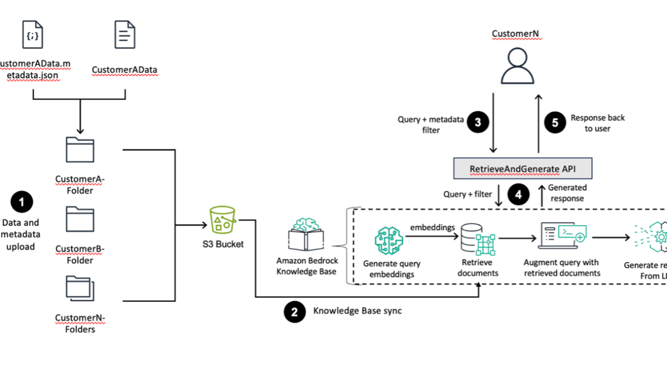
Shreyas Subramanian is a Principal Data Scientist and helps customers by using generative AI and deep learning to solve their business challenges using AWS services. Shreyas has a background in large-scale optimization and ML and in the use of ML and reinforcement learning for accelerating optimization tasks.

Satveer Khurpa is a Sr. WW Specialist Solutions Architect, Amazon Bedrock at Amazon Web Services, specializing in Amazon Bedrock security. In this role, he uses his expertise in cloud-based architectures to develop innovative generative AI solutions for clients across diverse industries. Satveer’s deep understanding of generative AI technologies and security principles allows him to design scalable, secure, and responsible applications that unlock new business opportunities and drive tangible value while maintaining robust security postures.

Kosta Belz is a Senior Applied Scientist in the AWS Generative AI Innovation Center, where he helps customers design and build generative AI solutions to solve key business problems.

Sean Eichenberger is a Sr Product Manager at AWS.

Read More