Digitizing Smell: Using Molecular Maps to Understand Odor

Posted by Richard C. Gerkin, Google Research, and Alexander B. Wiltschko, Google

How can we measure a smell? Smells are produced by molecules that waft through the air, enter our noses, and bind to sensory receptors. Potentially billions of molecules can produce a smell, so figuring out which ones produce which smells is difficult to catalog or predict. Sensory maps can help us solve this problem. Color vision has the most familiar examples of these maps, from the color wheel we each learn in primary school to more sophisticated variants used to perform color correction in video production. While these maps have existed for centuries, useful maps for smell have been missing, because smell is a harder problem to crack: molecules vary in many more ways than photons do; data collection requires physical proximity between the smeller and smell (we don’t have good smell “cameras” and smell “monitors”); and the human eye only has three sensory receptors for color while the human nose has > 300 for odor. As a result, previous efforts to produce odor maps have failed to gain traction.

In 2019, we developed a graph neural network (GNN) model that began to explore thousands of examples of distinct molecules paired with the smell labels that they evoke, e.g., “beefy”, “floral”, or “minty”, to learn the relationship between a molecule’s structure and the probability that such a molecule would have each smell label. The embedding space of this model contains a representation of each molecule as a fixed-length vector describing that molecule in terms of its odor, much as the RGB value of a visual stimulus describes its color.

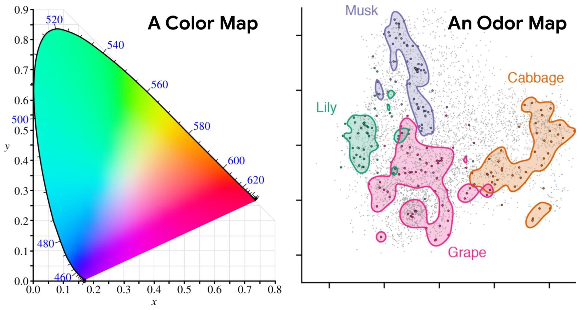
Left: An example of a color map (CIE 1931) in which coordinates can be directly translated into values for hue and saturation. Similar colors lie near each other, and specific wavelengths of light (and combinations thereof) can be identified with positions on the map. Right: Odors in the Principal Odor Map operate similarly. Individual molecules correspond to points (grey), and the locations of these points reflect predictions of their odor character.

Today we introduce the “Principal Odor Map” (POM), which identifies the vector representation of each odorous molecule in the model’s embedding space as a single point in a high-dimensional space. The POM has the properties of a sensory map: first, pairs of perceptually similar odors correspond to two nearby points in the POM (by analogy, red is nearer to orange than to green on the color wheel). Second, the POM enables us to predict and discover new odors and the molecules that produce them. In a series of papers, we demonstrate that the map can be used to prospectively predict the odor properties of molecules, understand these properties in terms of fundamental biology, and tackle pressing global health problems. We discuss each of these promising applications of the POM and how we test them below.

Test 1: Challenging the Model with Molecules Never Smelled Before
First, we asked if the underlying model could correctly predict the odors of new molecules that no one had ever smelled before and that were very different from molecules used during model development. This is an important test — many models perform well on data that looks similar to what the model has seen before, but break down when tested on novel cases.

To test this, we collected the largest ever dataset of odor descriptions for novel molecules. Our partners at the Monell Center trained panelists to rate the smell of each of 400 molecules using 55 distinct labels (e.g., “minty”) that were selected to cover the space of possible smells while being neither redundant nor too sparse. Unsurprisingly, we found that different people had different characterizations of the same molecule. This is why sensory research typically uses panels of dozens or hundreds of people and highlights why smell is a hard problem to solve. Rather than see if the model could match any one person, we asked how close it was to the consensus: the average across all of the panelists. We found that the predictions of the model were closer to the consensus than the average panelist was. In other words, the model demonstrated an exceptional ability to predict odor from a molecule’s structure.

<!–

Predictions made by two models, our GNN model (orange) and a baseline chemoinformatic random forest (RF) model (blue), compared with the mean ratings given by trained panelists (green) for the molecule 2,3-dihydrobenzofuran-5-carboxaldehyde. Each bar corresponds to one odor character label (with only the top 17 of 55 shown for clarity). The top five are indicated in color; our model correctly identifies four of the top five, with high confidence, vs. only three of five, with low confidence, for the RF model. The correlation (R) to the full set of 55 labels is also higher in our model.

–>

<!–

Unlike alternative benchmark models (RF and nearest-neighbor models trained on various sets of chemoinformatic features), our GNN model outperforms the median human panelist at predicting the panel mean rating. In other words, our GNN model better reflects the panel consensus than the typical panelist.

–>

The POM also exhibited state-of-the-art performance on alternative human olfaction tasks like detecting the strength of a smell or the similarity of different smells. Thus, with the POM, it should be possible to predict the odor qualities of any of billions of as-yet-unknown odorous molecules, with broad applications to flavor and fragrance.

Test 2: Linking Odor Quality Back to Fundamental Biology
Because the Principal Odor Map was useful in predicting human odor perception, we asked whether it could also predict odor perception in animals, and the brain activity that underlies it. We found that the map could successfully predict the activity of sensory receptors, neurons, and behavior in most animals that olfactory neuroscientists have studied, including mice and insects.

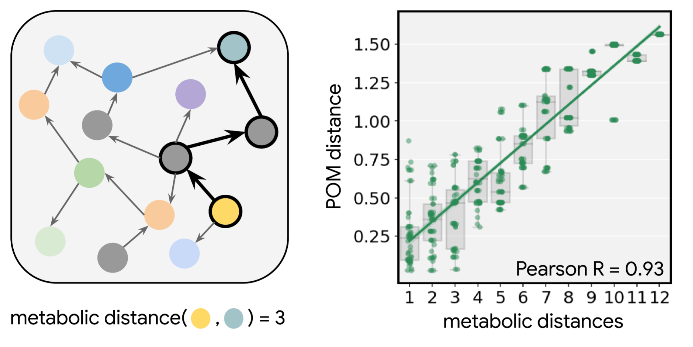
What common feature of the natural world makes this map applicable to species separated by hundreds of millions of years of evolution? We realized that the common purpose of the ability to smell might be to detect and discriminate between metabolic states, i.e., to sense when something is ripe vs. rotten, nutritious vs. inert, or healthy vs. sick. We gathered data about metabolic reactions in dozens of species across the kingdoms of life and found that the map corresponds closely to metabolism itself. When two molecules are far apart in odor, according to the map, a long series of metabolic reactions is required to convert one to the other; by contrast, similarly smelling molecules are separated by just one or a few reactions. Even long reaction pathways containing many steps trace smooth paths through the map. And molecules that co-occur in the same natural substances (e.g., an orange) are often very tightly clustered on the map. The POM shows that olfaction is linked to our natural world through the structure of metabolism and, perhaps surprisingly, captures fundamental principles of biology.

Left: We aggregated metabolic reactions found in 17 species across 4 kingdoms to construct a metabolic graph. In this illustration, each circle is a distinct metabolite molecule and an arrow indicates that there is a metabolic reaction that converts one molecule to another. Some metabolites have an odor (color) and others do not (gray), and the metabolic distance between two odorous metabolites is the minimum number of reactions necessary to convert one into the other. In the path shown in bold, the distance is 3. Right: Metabolic distance was highly correlated with distance in the POM, an estimate of perceived odor dissimilarity.

<!–

Left: We aggregated metabolic reactions found in 17 species across 4 kingdoms to construct a metabolic graph. In this illustration, each circle is a distinct metabolite molecule and an arrow indicates that there is a metabolic reaction that converts one molecule to another. Some metabolites have an odor (color) and others do not (gray), and the metabolic distance between two odorous metabolites is the minimum number of reactions necessary to convert one into the other. In the path shown in bold, the distance is 3. Right: Metabolic distance was highly correlated with distance in the POM, an estimate of perceived odor dissimilarity.

–>

Test 3: Extending the Model to Tackle a Global Health Challenge
A map of odor that is tightly connected to perception and biology across the animal kingdom opens new doors. Mosquitos and other insect pests are drawn to humans in part by their odor perception. Since the POM can be used to predict animal olfaction generally, we retrained it to tackle one of humanity’s biggest problems, the scourge of diseases transmitted by mosquitoes and ticks, which kill hundreds of thousands of people each year.

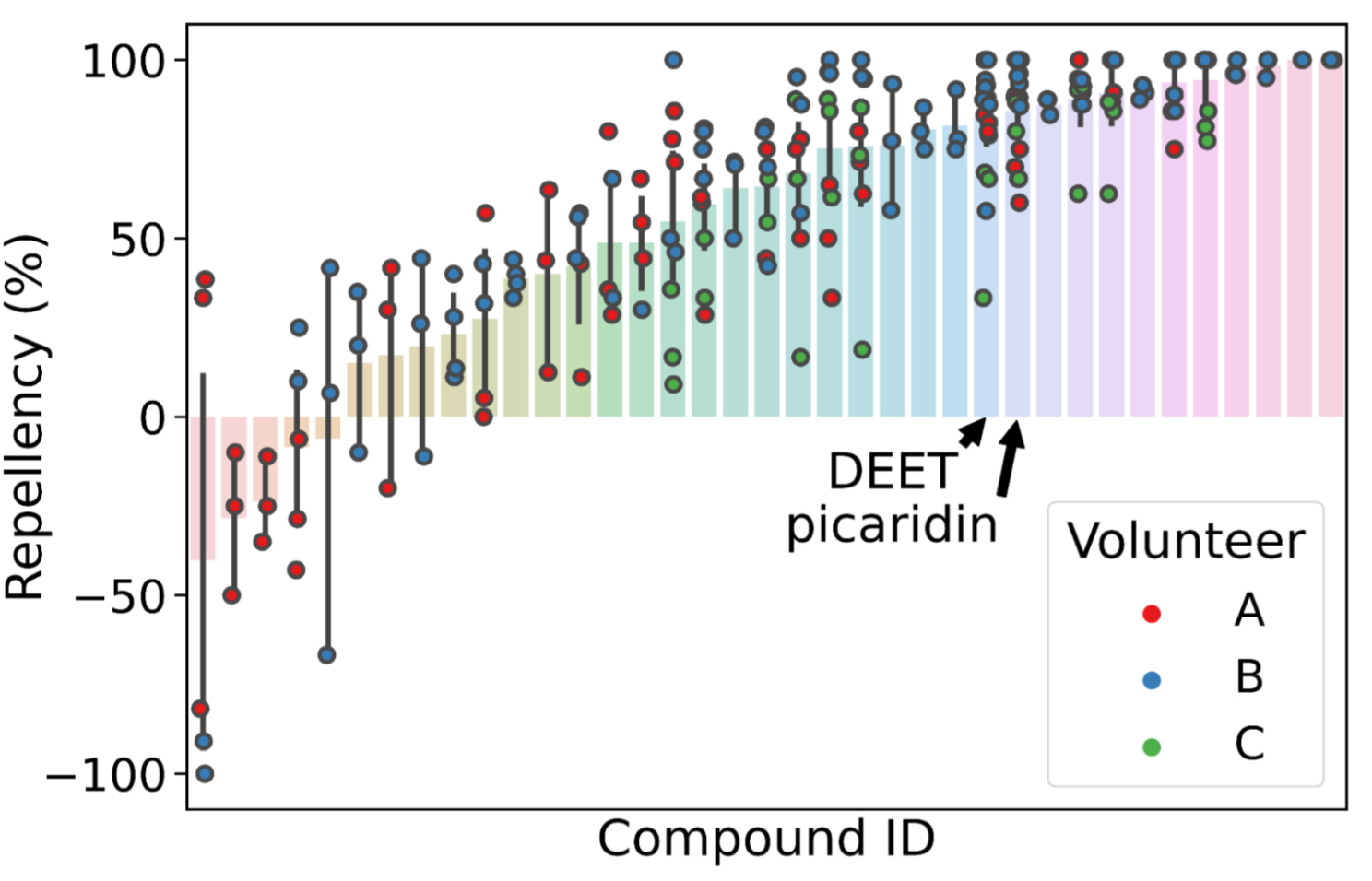
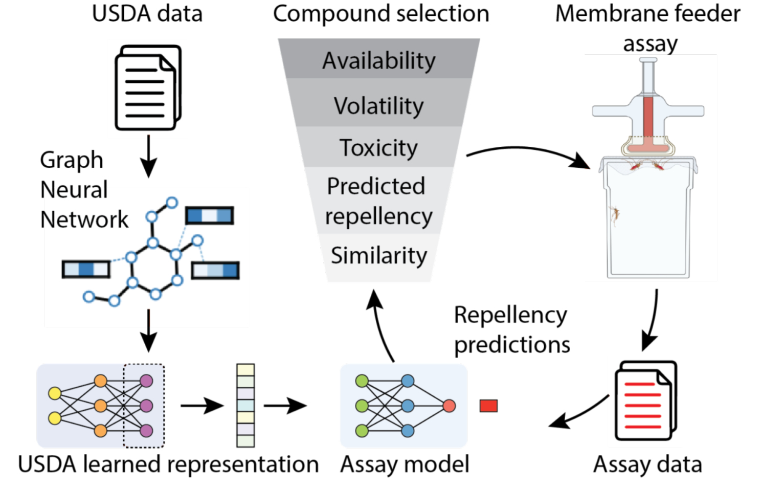
For this purpose, we improved our original model with two new sources of data: (1) a long-forgotten set of experiments conducted by the USDA on human volunteers beginning 80 years ago and recently made discoverable by Google Books, which we subsequently made machine-readable; and (2) a new dataset collected by our partners at TropIQ, using their high-throughput laboratory mosquito assay. Both datasets measure how well a given molecule keeps mosquitos away. Together, the resulting model can predict the mosquito repellency of nearly any molecule, enabling a virtual screen over huge swaths of molecular space. We validated this screen experimentally using entirely new molecules and found over a dozen of them with repellency at least as high as DEET, the active ingredient in most insect repellents. Less expensive, longer lasting, and safer repellents can reduce the worldwide incidence of diseases like malaria, potentially saving countless lives.

We digitized USDA mosquito repellency data for thousands of molecules previously scanned by Google Books, and used it to refine the learned representation (the map) at the heart of the model. We added additional layers, specifically to predict repellency in a mosquito feeder assay, and iteratively trained the model to improve assay predictions while running computational screens for candidate repellents.

Many molecules showing mosquito repellency in the laboratory assay also showed repellency when applied to humans. Several showed repellency greater than the most common repellents used today (DEET and picaridin).

The Road Ahead
We discovered that our modeling approach to smell prediction could be used to draw a Principal Odor Map for tackling odor-related problems more generally. This map was the key to measuring smell: it answered a range of questions about novel smells and the molecules that produce them, it connected smells back to their origins in evolution and the natural world, and it is helping us tackle important human-health challenges that affect millions of people. Going forward, we hope that this approach can be used to find new solutions to problems in food and fragrance formulation, environmental quality monitoring, and the detection of human and animal diseases.

Acknowledgements
This work was performed by the ML olfaction research team, including Benjamin Sanchez-Lengeling, Brian K. Lee, Jennifer N. Wei, Wesley W. Qian, and Jake Yasonik (the latter two were partly supported by the Google Student Researcher program) and our external partners including Emily Mayhew and Joel D. Mainland from the Monell Center, and Koen Dechering and Marnix Vlot from TropIQ. The Google Books team brought the USDA dataset online. Richard C. Gerkin was supported by the Google Visiting Faculty Researcher program and is also an Associate Research Professor at Arizona State University.

Read More