Train self-supervised vision transformers on overhead imagery with Amazon SageMaker

This is a guest blog post co-written with Ben Veasey, Jeremy Anderson, Jordan Knight, and June Li from Travelers.

Satellite and aerial images provide insight into a wide range of problems, including precision agriculture, insurance risk assessment, urban development, and disaster response. Training machine learning (ML) models to interpret this data, however, is bottlenecked by costly and time-consuming human annotation efforts. One way to overcome this challenge is through self-supervised learning (SSL). By training on large amounts of unlabeled image data, self-supervised models learn image representations that can be transferred to downstream tasks, such as image classification or segmentation. This approach produces image representations that generalize well to unseen data and reduces the amount of labeled data required to build performant downstream models.

In this post, we demonstrate how to train self-supervised vision transformers on overhead imagery using Amazon SageMaker. Travelers collaborated with the Amazon Machine Learning Solutions Lab (now known as the Generative AI Innovation Center) to develop this framework to support and enhance aerial imagery model use cases. Our solution is based on the DINO algorithm and uses the SageMaker distributed data parallel library (SMDDP) to split the data over multiple GPU instances. When pre-training is complete, the DINO image representations can be transferred to a variety of downstream tasks. This initiative led to improved model performances within the Travelers Data & Analytics space.

Overview of solution

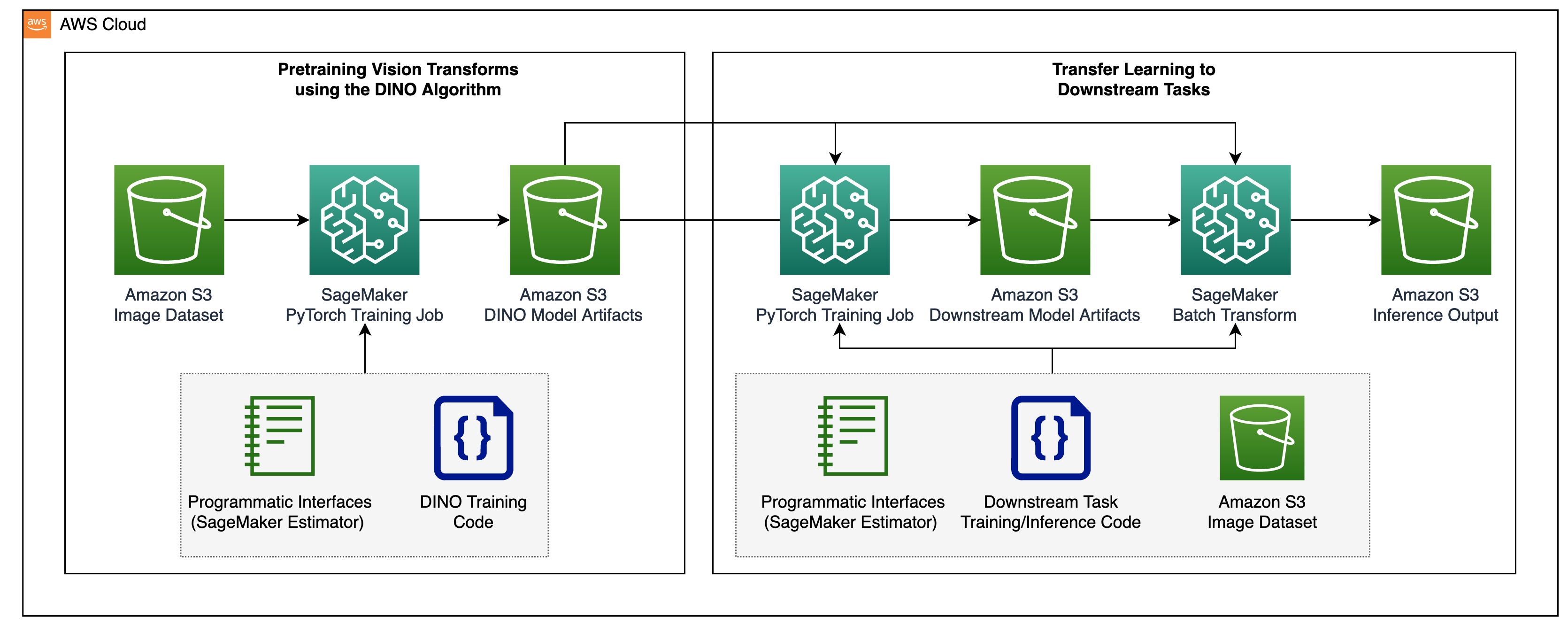
The two-step process for pre-training vision transformers and transferring them to supervised downstream tasks is shown in the following diagram.

In the following sections, we provide a walkthrough of the solution using satellite images from the BigEarthNet-S2 dataset. We build on the code provided in the DINO repository.

Prerequisites

Before getting started, you need access to a SageMaker notebook instance and an Amazon Simple Storage Service (Amazon S3) bucket.

Prepare the BigEarthNet-S2 dataset

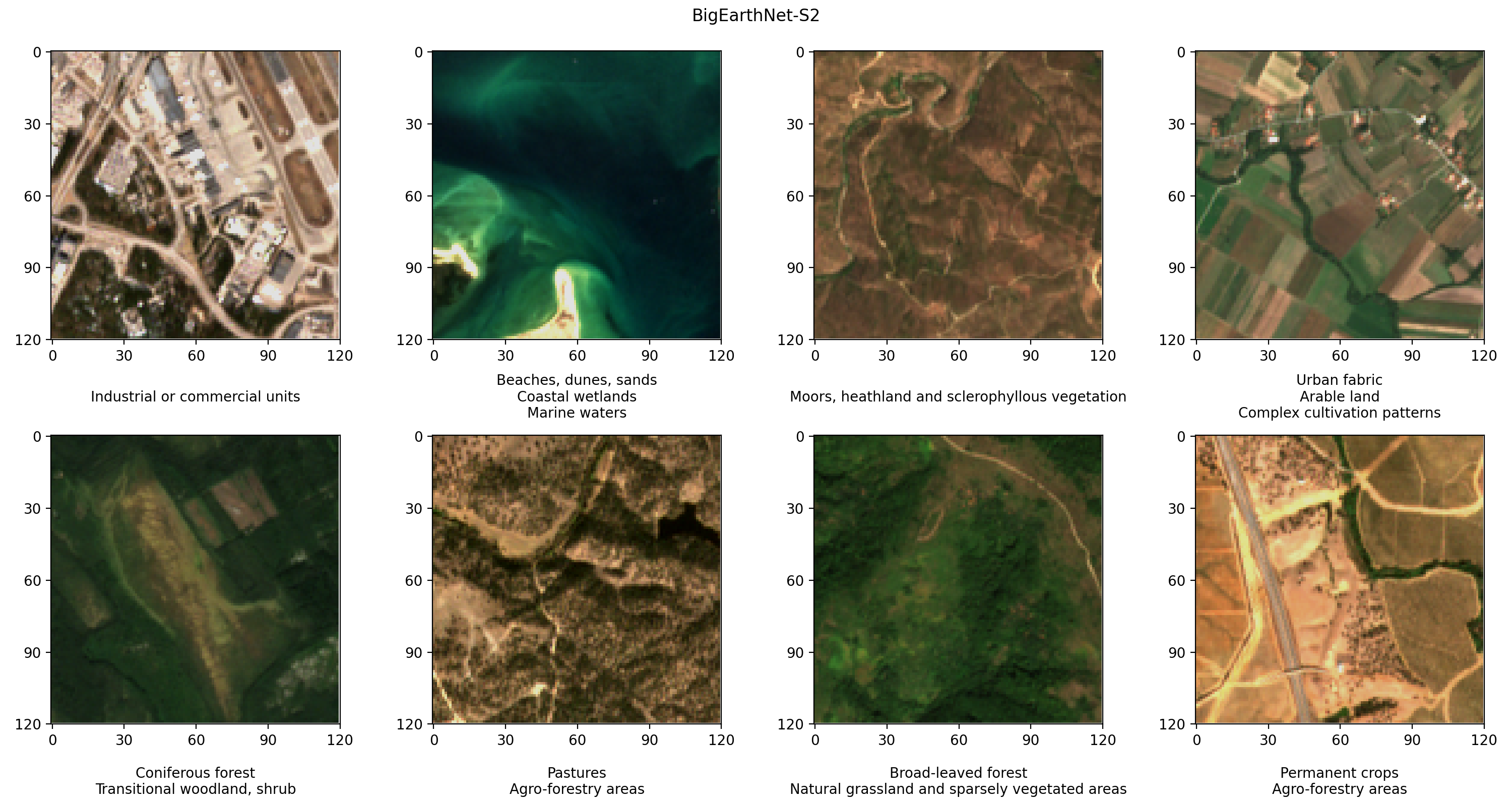
BigEarthNet-S2 is a benchmark archive that contains 590,325 multispectral images collected by the Sentinel-2 satellite. The images document the land cover, or physical surface features, of ten European countries between June 2017 and May 2018. The types of land cover in each image, such as pastures or forests, are annotated according to 19 labels. The following are a few example RGB images and their labels.

The first step in our workflow is to prepare the BigEarthNet-S2 dataset for DINO training and evaluation. We start by downloading the dataset from the terminal of our SageMaker notebook instance:

wget https://bigearth.net/downloads/BigEarthNet-S2-v1.0.tar.gz
tar -xvf BigEarthNet-S2-v1.0.tar.gz

The dataset has a size of about 109 GB. Each image is stored in its own folder and contains 12 spectral channels. Three bands with 60m spatial resolution (60-meter pixel height/width) are designed to identify aerosols (B01), water vapor (B09), and clouds (B10). Six bands with 20m spatial resolution are used to identify vegetation (B05, B06, B07, B8A) and distinguish between snow, ice, and clouds (B11, B12). Three bands with 10m spatial resolution help capture visible and near-infrared light (B02, B03, B04, B8/B8A). Additionally, each folder contains a JSON file with the image metadata. A detailed description of the data is provided in the BigEarthNet Guide.

To perform statistical analyses of the data and load images during DINO training, we process the individual metadata files into a common geopandas Parquet file. This can be done using the BigEarthNet Common and the BigEarthNet GDF Builder helper packages:

python -m bigearthnet_gdf_builder.builder build-recommended-s2-parquet BigEarthNet-v1.0/

The resulting metadata file contains the recommended image set, which excludes 71,042 images that are fully covered by seasonal snow, clouds, and cloud shadows. It also contains information on the acquisition date, location, land cover, and train, validation, and test split for each image.

We store the BigEarthNet-S2 images and metadata file in an S3 bucket. Because we use true color images during DINO training, we only upload the red (B04), green (B03), and blue (B02) bands:

aws s3 cp final_ben_s2.parquet s3://bigearthnet-s2-dataset/metadata/
aws s3 cp BigEarthNet-v1.0/ s3://bigearthnet-s2-dataset/data_rgb/ 
    --recursive 
    --exclude "*" 
    --include "_B02.tif" 
    --include "_B03.tif"  
    --include "_B04.tif"

The dataset is approximately 48 GB in size and has the following structure:

bigearthnet-s2-dataset/                                    Amazon S3 bucket
├── metadata/
│ └── final_ben_s2.parquet 
└── dataset_rgb/
  ├── S2A_MSIL2A_20170613T101031_0_45/
  │ └── S2A_MSIL2A_20170613T101031_0_45_B02.tif            Blue channel
  │ └── S2A_MSIL2A_20170613T101031_0_45_B03.tif            Green channel
  │ └── S2A_MSIL2A_20170613T101031_0_45_B04.tif            Red channel

Train DINO models with SageMaker

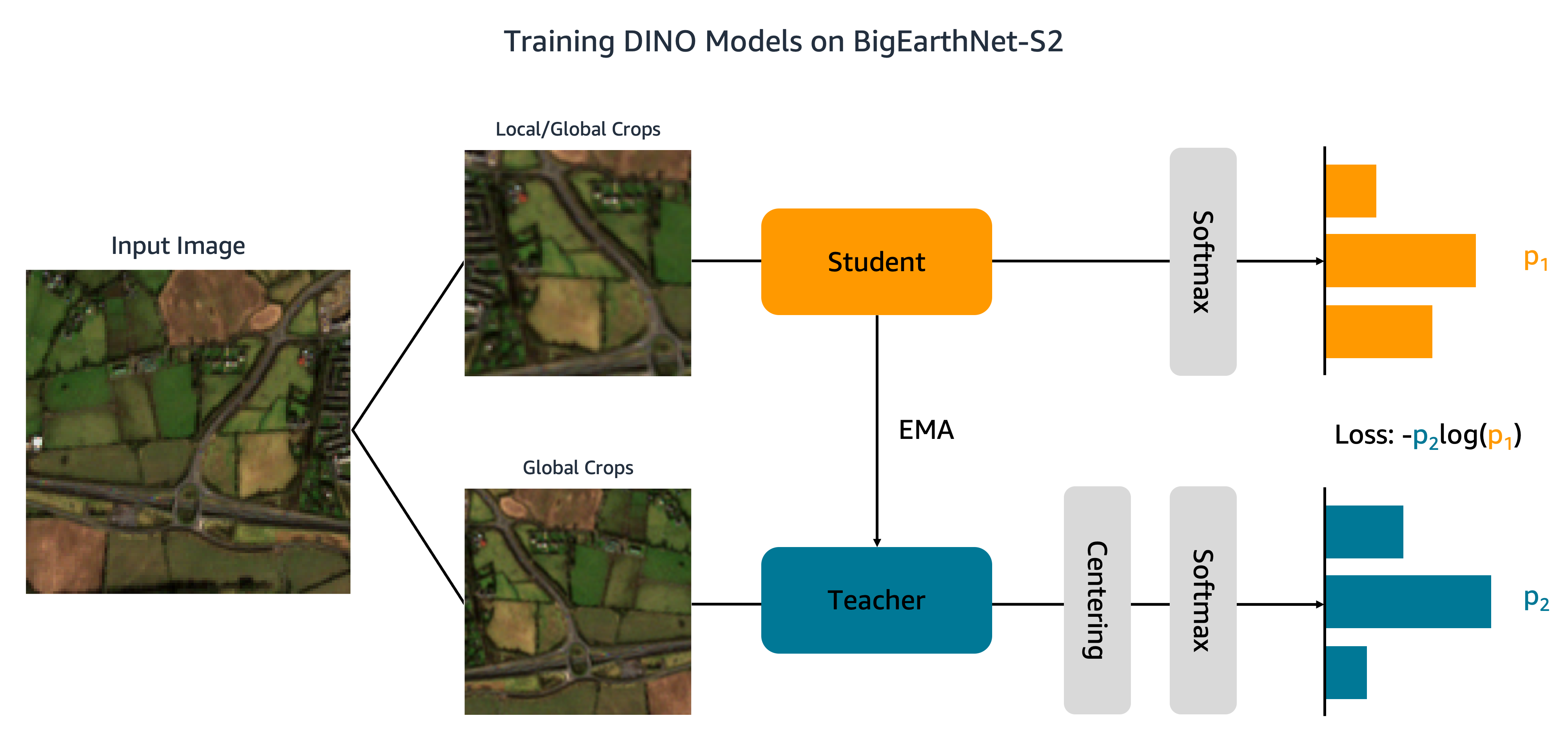
Now that our dataset has been uploaded to Amazon S3, we move to train DINO models on BigEarthNet-S2. As shown in the following figure, the DINO algorithm passes different global and local crops of an input image to student and teacher networks. The student network is taught to match the output of the teacher network by minimizing the cross-entropy loss. The student and teacher weights are connected by an exponential moving average (EMA).

We make two modifications to the original DINO code. First, we create a custom PyTorch dataset class to load the BigEarthNet-S2 images. The code was initially written to process ImageNet data and expects images to be stored by class. BigEarthNet-S2, however, is a multi-label dataset where each image resides in its own subfolder. Our dataset class loads each image using the file path stored in the metadata:

import pandas as pd
import rasterio
from PIL import Image
import torch
from torch.utils.data import Dataset, DataLoader
from torchvision import transforms, utils
 
OPTICAL_MAX_VALUE = 2000

LAND_COVER_LABELS = [
    "Urban fabric",
    "Industrial or commercial units",
    "Arable land",
    "Permanent crops",
    "Pastures",
    "Complex cultivation patterns",
    "Land principally occupied by agriculture, with significant areas of natural vegetation",
    "Agro-forestry areas",
    "Broad-leaved forest",
    "Coniferous forest",
    "Mixed forest",
    "Natural grassland and sparsely vegetated areas",
    "Moors, heathland and sclerophyllous vegetation",
    "Transitional woodland, shrub",
    "Beaches, dunes, sands",
    "Inland wetlands",
    "Coastal wetlands",
    "Inland waters",
    "Marine waters",
]
 
class BigEarthNetDataset(Dataset):
     """
     PyTorch dataset class that loads the BigEarthNet-S2 images from a metadata file.

     Args: 
          metadata_file: path to metadata file 
          data_dir: directory where BigEarthNet-S2 data is located  
          split: train, validation, or test split
          transform: transformations applied to the input image
     """
     def __init__(self, metadata_file, data_dir, split="train", transform=None):
		# image file paths from metadata
        metadata = pd.read_parquet(metadata_file)
        self.metadata_split = metadata[metadata["original_split"] == split]
        self.data_dir = data_dir
        self.patch_names = self.metadata_split["name"].tolist()
 
        # one-hot-encode land cover labels 
        multiclass_labels = self.metadata_split.new_labels.tolist()
        self.labels = self.get_multi_onehot_labels(multiclass_labels)

        # transforms        
        self.transform = transform
 
    def __len__(self):
        """Return length of dataset."""
        return len(self.metadata_split)
 
    def __getitem__(self, index):
        """Returns the image and label for a given index."""
        patch_name = self.patch_names[index]
        file_path = os.path.join(self.data_dir, patch_name)
	
	# generate RGB image
        r_channel = rasterio.open(os.path.join(file_path, patch_name + "_B04.tif")).read(1)
        g_channel = rasterio.open(os.path.join(file_path, patch_name + "_B03.tif")).read(1)
        b_channel = rasterio.open(os.path.join(file_path, patch_name + "_B02.tif")).read(1)
 
        image = np.stack([r_channel, g_channel, b_channel], axis=2)
        image = image / OPTICAL_MAX_VALUE * 255
        image = np.clip(image, 0, 225).astype(np.uint8)
    
        # apply image transforms
        image = Image.fromarray(image, mode="RGB")
        if self.transform is not None:
            image = self.transform(image)
 
        # load label
        label = self.labels[index]
 
        return image, label
  
    def get_multi_onehot_labels(self, multiclass_labels):
        """Convert BEN-19 labels to one-hot encoded vector."""
        targets = torch.zeros([len(multiclass_labels), len(LAND_COVER_LABELS)])
        for index, img_labels in enumerate(multiclass_labels):
            for label in img_labels:
                index_hot = LAND_COVER_LABELS.index(label)
                targets[index, index_hot] = 1.
        return targets

This dataset class is called in main_dino.py during training. Although the code includes a function to one-hot encode the land cover labels, these labels are not used by the DINO algorithm.

The second change we make to the DINO code is to add support for SMDDP. We add the following code to the init_distributed_mode function in the util.py file:

init_distributed_mode function in the util.py file:

def init_distributed_mode(args):
     if json.loads(
          os.environ.get('SM_FRAMEWORK_PARAMS', '{}'))
         .get('sagemaker_distributed_dataparallel_enabled', False)
     ): 
          # launch training with SMDDP 
          dist.init_process_group(backend='smddp')
          args.word_size = dist.get_world_size() 
          args.gpu = int(os.environ['LOCAL_RANK'])

With these adjustments, we are ready to train DINO models on BigEarthNet-S2 using SageMaker. To train on multiple GPUs or instances, we create a SageMaker PyTorch Estimator that ingests the DINO training script, the image and metadata file paths, and the training hyperparameters:

import time
from sagemaker.pytorch import PyTorch

# output bucket where final model artifacts are uploaded 
DINO_OUTPUT_BUCKET = 'dino-models'

# paths on training instance  
sm_metadata_path = '/opt/ml/input/data/metadata'              
sm_data_path = '/opt/ml/input/data/train'                     
sm_output_path = '/opt/ml/output/data'                        
sm_checkpoint_path = '/opt/ml/checkpoints'                

# training job name
dino_base_job_name = f'dino-model-{int(time.time())}'

# create SageMaker Estimator
estimator = PyTorch(
    base_job_name=dino_base_job_name,
    source_dir='path/to/aerial_featurizer',
    entry_point='main_dino.py',
    role=role,
    framework_version="1.12",
    py_version="py38",
    instance_count=1,
    instance_type="ml.p3.16xlarge",    
    distribution = {'smdistributed':{'dataparallel':{'enabled': True}}},        
    volume_size=100,
    sagemaker_session=sagemaker_session,
    hyperparameters = {
        # hyperparameters passed to entry point script
        'arch': 'vit_small',
        'patch_size': 16,
        'metadata_dir': sm_metadata_path,
        'data_dir': sm_data_path,
        'output_dir': sm_output_path,
        'checkpoint_dir': sm_checkpoint_path,
        'epochs': 100,
        'saveckp_freq': 20,
    },
    max_run=24*60*60,               
    checkpoint_local_path = sm_checkpoint_path,
    checkpoint_s3_uri =f's3://{DINO_OUTPUT_BUCKET}/checkpoints/{base_job_name}', 
    debugger_hook_config=False,                           
)

This code specifies that we will train a small vision transformer model (21 million parameters) with a patch size of 16 for 100 epochs. It is best practice to create a new checkpoint_s3_uri for each training job in order to reduce the initial data download time. Because we are using SMDDP, we must train on an ml.p3.16xlarge, ml.p3dn.24xlarge, or ml.p4d.24xlarge instance. This is because SMDDP is only enabled for the largest multi-GPU instances. To train on smaller instance types without SMDDP, you will need to remove the distribution and debugger_hook_config arguments from the estimator.

After we have created the SageMaker PyTorch Estimator, we launch the training job by calling the fit method. We specify the input training data using the Amazon S3 URIs for the BigEarthNet-S2 metadata and images:

# call fit to begin training
estimator.fit(
    inputs={
        'metadata': 's3://bigearthnet-s2-dataset/metadata/',
        'train': 's3://bigearthnet-s2-dataset/data_rgb/',
    },
    wait=False
)

SageMaker spins up the instance, copies the training script and dependencies, and begins DINO training. We can monitor the progress of the training job from our Jupyter notebook using the following commands:

# monitor training
training_job_name = estimator.latest_training_job.name 
attached_estimator = PyTorch.attach(training_job_name)
attached_estimator.logs()

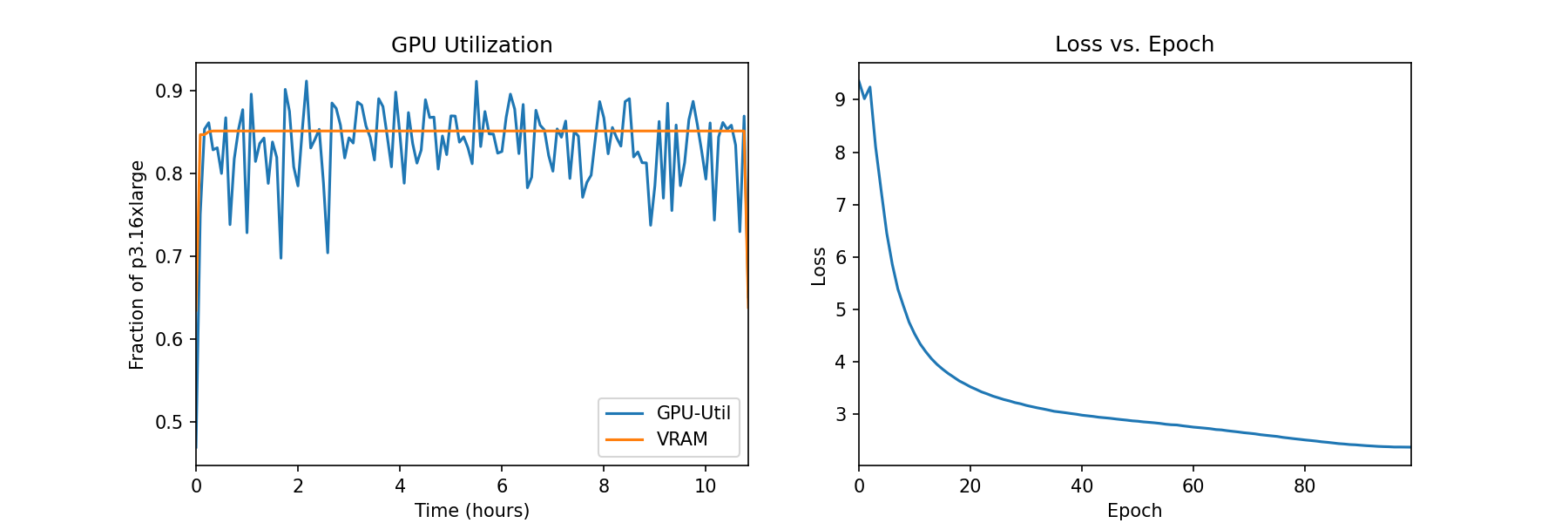
We can also monitor instance metrics and view log files on the SageMaker console under Training jobs. In the following figures, we plot the GPU utilization and loss function for a DINO model trained on an ml.p3.16xlarge instance with a batch size of 128.

During training, the GPU utilization is 83% of the ml.p3.16xlarge capacity (8 NVIDIA Tesla V100 GPUs) and the VRAM usage is 85%. The loss function steadily decreases with each epoch, indicating that the outputs of the student and teacher networks are becoming more similar. In total, training takes about 11 hours.

Transfer learning to downstream tasks

Our trained DINO model can be transferred to downstream tasks like image classification or segmentation. In this section, we use the pre-trained DINO features to predict the land cover classes for images in the BigEarthNet-S2 dataset. As depicted in the following diagram, we train a multi-label linear classifier on top of frozen DINO features. In this example, the input image is associated with arable land and pasture land covers.

Most of the code for the linear classifier is already in place in the original DINO repository. We make a few adjustments for our specific task. As before, we use the custom BigEarthNet dataset to load images during training and evaluation. The labels for the images are one-hot encoded as 19-dimensional binary vectors. We use the binary cross-entropy for the loss function and compute the average precision to evaluate the performance of the model.

To train the classifier, we create a SageMaker PyTorch Estimator that runs the training script, eval_linear.py. The training hyperparameters include the details of the DINO model architecture and the file path for the model checkpoint:

# output bucket where final model artifacts are uploaded 
CLASSIFIER_OUTPUT_BUCKET = 'land-cover-classification'

# DINO checkpoint name 
checkpoint = 'checkpoint.pth'

# paths on training instance  
sm_dino_path = f'/opt/ml/input/data/dino_checkpoint'          
sm_dino_checkpoint = f'{sm_dino_path}/{checkpoint}'           

# training job name
classifier_base_job_name = f'linear-classifier-{int(time.time())}'

# create Estimator 
estimator = PyTorch(
    base_job_name=classifier_base_job_name,
    source_dir='path/to/aerial_featurizer',
    entry_point = 'eval_linear.py',
    role=role,
    framework_version='1.12',
    py_version='py38',
    instance_count=1,
    instance_type='ml.p3.2xlarge',
    sagemaker_session=sagemaker_session,
    hyperparameters = {
    # hyperparameters passed to entry point script
        'arch': 'vit_small',
        'pretrained_weights': sm_dino_checkpoint,
        'epochs': 50,
        'data_dir': sm_data_path,
        'metadata_dir': sm_metadata_path,
        'output_dir': sm_checkpoint_path,
        'num_labels': 19,
    },
    max_run=1*60*60, 
    checkpoint_local_path = sm_checkpoint_path,
    checkpoint_s3_uri =f's3://{CLASSIFIER_OUTPUT_BUCKET}/checkpoints/{base_job_name}',
)

We start the training job using the fit method, supplying the Amazon S3 locations of the BigEarthNet-S2 metadata and training images and the DINO model checkpoint:

# call fit to begin training
estimator.fit(
    inputs={
    'metadata': 's3://bigearthnet-s2-dataset/metadata/',
    'dataset': 's3://bigearthnet-s2-dataset/data_rgb/',
    'dino_checkpoint': f's3://bigearthnet-s2-dataset/dino-models/checkpoints/{dino_base_job_name}',
    },
    wait=False
)

When training is complete, we can perform inference on the BigEarthNet-S2 test set using SageMaker batch transform or SageMaker Processing. In the following table, we compare the average precision of the linear model on test set images using two different DINO image representations. The first model, ViT-S/16 (ImageNet), is the small vision transformer checkpoint included in the DINO repository that was pre-trained using front-facing images in the ImageNet dataset. The second model, ViT-S/16 (BigEarthNet-S2), is the model we produced by pre-training on overhead imagery.

We find that the DINO model pre-trained on BigEarthNet-S2 transfers better to the land cover classification task than the DINO model pre-trained on ImageNet, resulting in a 6.7% increase in the average precision.

Clean up

After completing DINO training and transfer learning, we can clean up our resources to avoid incurring charges. We stop or delete our notebook instance and remove any unwanted data or model artifacts from Amazon S3.

Conclusion

This post demonstrated how to train DINO models on overhead imagery using SageMaker. We used SageMaker PyTorch Estimators and SMDDP in order to generate representations of BigEarthNet-S2 images without the need for explicit labels. We then transferred the DINO features to a downstream image classification task, which involved predicting the land cover class of BigEarthNet-S2 images. For this task, pre-training on satellite imagery yielded a 6.7% increase in average precision relative to pre-training on ImageNet.

You can use this solution as a template for training DINO models on large-scale, unlabeled aerial and satellite imagery datasets. To learn more about DINO and building models on SageMaker, check out the following resources:

• Emerging Properties in Self-Supervised Vision Transformers
• Use PyTorch with Amazon SageMaker
• SageMaker’s Data Parallelism Library

About the Authors

Ben Veasey is a Senior Associate Data Scientist at Travelers, working within the AI & Automation Accelerator team. With a deep understanding of innovative AI technologies, including computer vision, natural language processing, and generative AI, Ben is dedicated to accelerating the adoption of these technologies to optimize business processes and drive efficiency at Travelers.

Jeremy Anderson is a Director & Data Scientist at Travelers on the AI & Automation Accelerator team. He is interested in solving business problems with the latest AI and deep learning techniques including large language models, foundational imagery models, and generative AI. Prior to Travelers, Jeremy earned a PhD in Molecular Biophysics from the Johns Hopkins University and also studied evolutionary biochemistry. Outside of work you can find him running, woodworking, or rewilding his yard.

Jordan Knight is a Senior Data Scientist working for Travelers in the Business Insurance Analytics & Research Department. His passion is for solving challenging real-world computer vision problems and exploring new state-of-the-art methods to do so. He has a particular interest in the social impact of ML models and how we can continue to improve modeling processes to develop ML solutions that are equitable for all. Jordan graduated from MIT with a Master’s in Business Analytics. In his free time you can find him either rock climbing, hiking, or continuing to develop his somewhat rudimentary cooking skills.

June Li is a data scientist at Travelers’s Business Insurance’s Artificial Intelligence team, where she leads and coordinates work in the AI imagery portfolio. She is passionate about implementing innovative AI solutions that bring substantial value to the business partners and stakeholders. Her work has been integral in transforming complex business challenges into opportunities by leveraging cutting-edge AI technologies.

Sourav Bhabesh is a Senior Applied Scientist at the AWS Titan Labs, where he builds Foundational Model (FM) capabilities and features. His specialty is Natural Language Processing (NLP) and is passionate about deep learning. Outside of work he enjoys reading books and traveling.

Laura Kulowski is an Applied Scientist at Amazon’s Generative AI Innovation Center, where she works closely with customers to build generative AI solutions. In her free time, Laura enjoys exploring new places by bike.

Andrew Ang is a Sr. Machine Learning Engineer at AWS. In addition to helping customers build AI/ML solutions, he enjoys water sports, squash and watching travel & food vlogs.

Mehdi Noori is an Applied Science Manager at the Generative AI Innovation Center. With a passion for bridging technology and innovation, he assists AWS customers in unlocking the potential of generative AI, turning potential challenges into opportunities for rapid experimentation and innovation by focusing on scalable, measurable, and impactful uses of advanced AI technologies, and streamlining the path to production.

Read More