As models scale in depth, batch size, and sequence length, etc, activation memory becomes an increasingly significant contributor to the overall memory usage. To help address this, PyTorch provides utilities for activation checkpointing, which reduce the number of saved tensors by recomputing them when needed, trading off memory usage for additional compute.
In this post, we’ll walk through the basics of what activation memory is, the high-level ideas behind existing activation checkpointing techniques, and also introduce some newer techniques that aim to improve flexibility and provide more optimization/automation out of the box.
As we look at these techniques, we’ll compare how these methods fit into a speed vs. memory trade-off diagram and hopefully provide some insight on how to choose the right strategy for your use case.
(If you prefer to jump straight to the new APIs, please skip ahead to the “Selective Activation Checkpoint” and “Memory Budget API” sections below.)
Activation Memory Basics
By default, in eager mode (rather than using torch.compile), PyTorch’s autograd preserves intermediate activations for backward computation. For example, if you call sin on a tensor x during the forward pass, autograd must remember x to compute cos(x) during backward.

If this tensor x is saved at the beginning of the forward pass, it remains in memory throughout both the forward and backward phases. It can only be cleared after it is used to compute the gradient, which happens at the end of the backward pass (due to the reverse order of execution).
Thus, as you proceed through the forward pass and perform more and more operations, you accumulate more and more activations, resulting in more and more activation memory until it (typically) reaches its peak at the start of backward (at which point activations can start to get cleared).
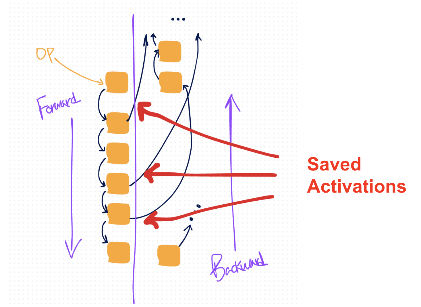
In the diagram above, the orange boxes represent operations, black arrows represent their tensor inputs and outputs. The black arrows that cross over the right represent tensors that autograd saves for backward.
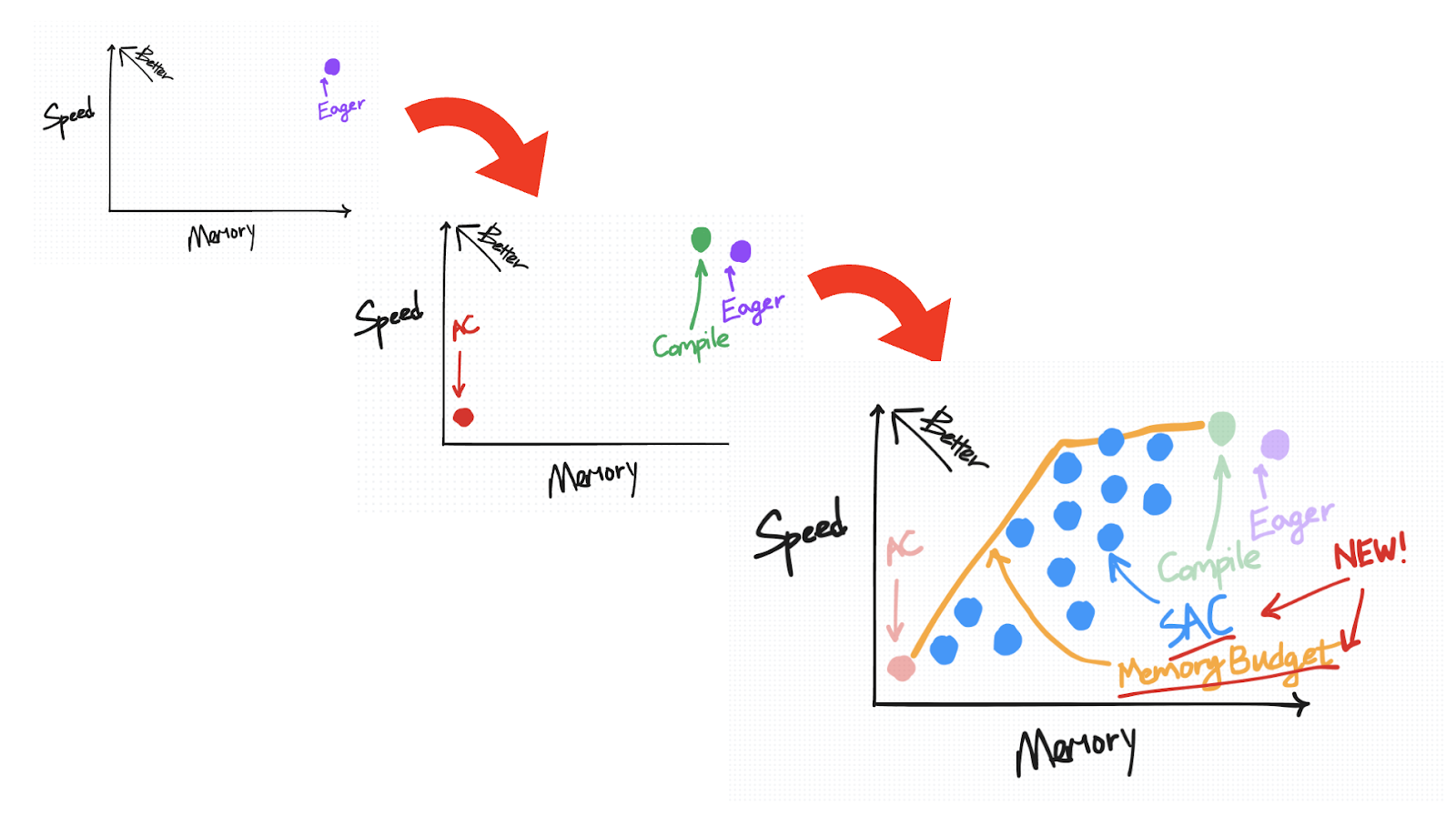
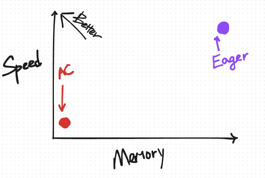
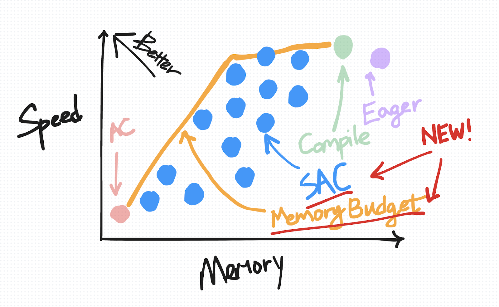
A useful way to visually organize this default saving behavior in eager as well as the techniques we’re about to introduce is based on how they trade off speed versus memory.
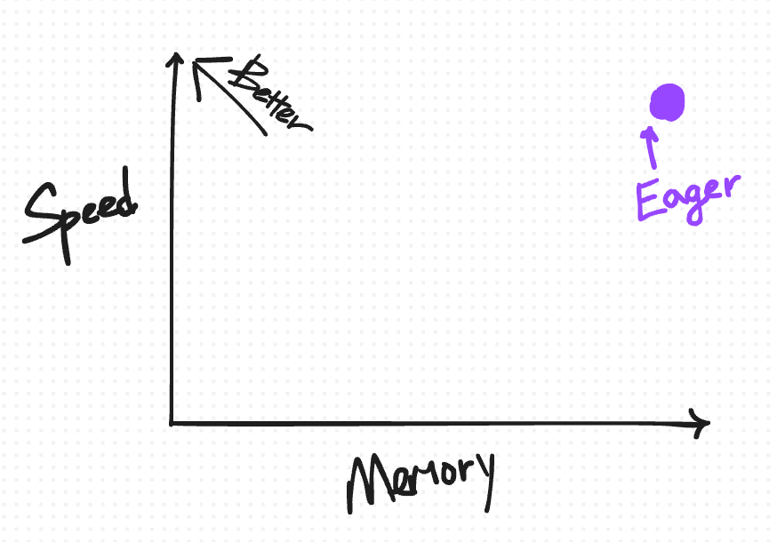
The ideal place to be on this diagram is the top-left, where you have “high” speed but also low memory usage.
We begin by putting the default saving behavior on the top-right (for reasons we’ll explain in more detail as we introduce more points for other techniques).
Activation Checkpointing (AC)
Activation checkpointing (AC) is a popular technique to reduce memory usage in PyTorch.
During forward, any operations performed inside the AC’d region do not save tensors for backward. (Only the inputs to the function are saved.) During backward, the intermediate activations needed for gradient computation are rematerialized by running the function a second time.
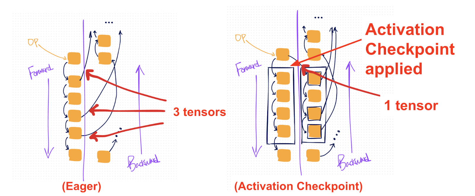
In the diagram (right), the black box shows where activation checkpointing is applied. Compared to the default eager approach (left), this setup results in fewer tensors being saved (1 versus 3).
Applying AC on the right parts of the model has the effect of reducing peak memory, because the intermediate activations are no longer materialized in memory when the memory usage typically peaks (at the beginning of backward).
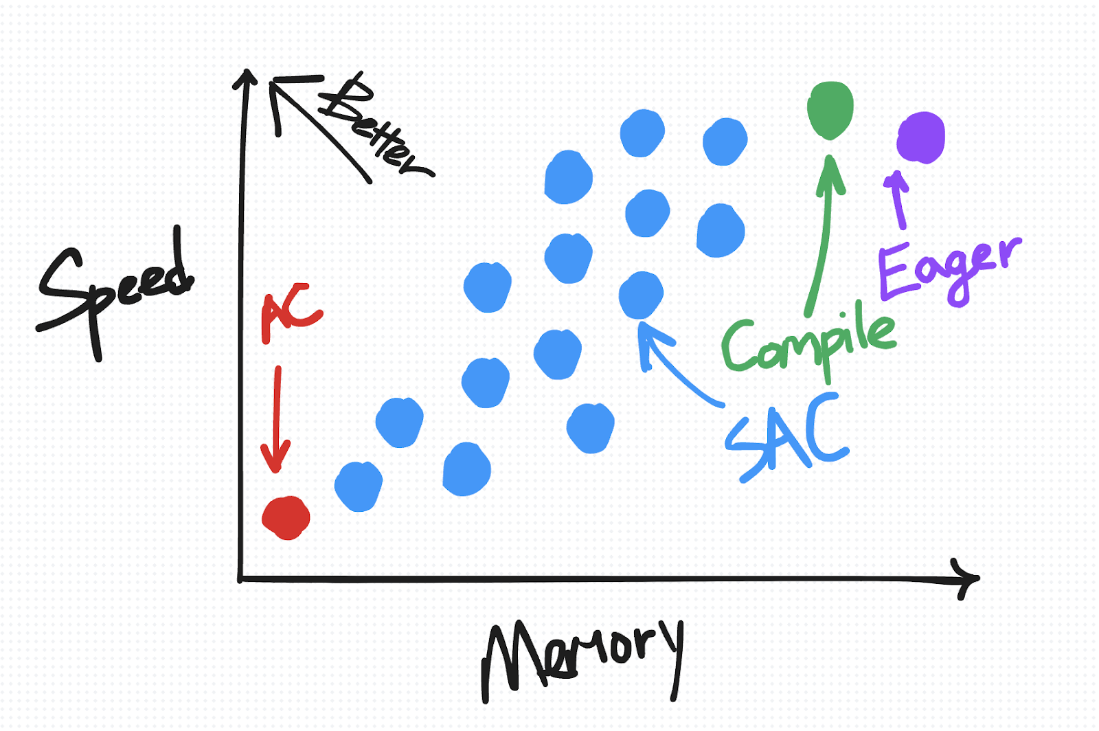
On the speed-versus-memory tradeoff diagram, AC is plotted on the bottom-left. Relative to eager mode, it reduces the amount of memory saved for backward but comes with an added cost in compute due to recomputation.
Note that AC’s speed–memory tradeoff /can/ be adjusted by selecting which parts of the forward pass to checkpoint and by defining how many checkpoint regions to use. However, implementing these changes may require modifying your model’s structure and can be cumbersome depending on how your code is organized. For the purposes of this diagram, we assume only one region is checkpointed; under this assumption, AC appears as a single point on the tradeoff diagram.
Also note that “memory” here does not refer to peak memory usage; rather, it indicates the how much memory is saved for backward for a fixed region.
torch.compile and min-cut partitioner
Another notable approach to keep in mind is torch.compile (introduced in PyTorch 2.0). Like activation checkpointing, torch.compile can also perform some level of recomputation under the hood. Specifically, it traces the forward and backward computations into a single joint graph, which is then processed by a “min-cut” partitioner. This partitioner uses a min-cut/max-flow algorithm to split the graph such that it minimizes the number of tensors that need to be saved for backward.
At first glance, this might sound a lot like what we want for activation memory reduction. However, the reality is more nuanced. By default, the partitioner’s primary goal is to reduce runtime. As a result, it only recomputes certain types of operations—primarily simpler, fusible, and non-compute-intensive ops (like pointwise ops).
Placing “compile” on the speed-versus-memory tradeoff diagram…
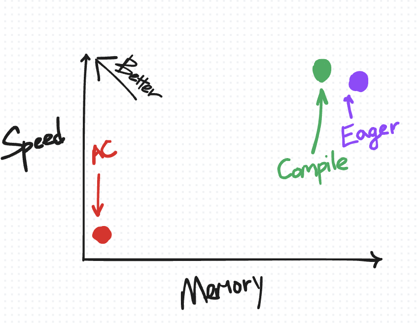
It is to the top-left of the eager non-AC point, as we expect torch.compile to improve on both speed and memory.
On the other hand, relative to activation checkpointing, torch.compile is more conservative about what it recomputes, placing it closer to the top-left on the speed-versus-memory diagram.
Selective Activation Checkpoint [NEW!]
While normal checkpointing recomputes every op in a chosen region, selective activation checkpointing (SAC) is an additional setting on top of activation checkpointing that you can apply to have a more granular control over which operations to recompute.
This can be useful if you have certain more expensive operations like matmuls which you prefer to avoid recomputing, but still generally want to recompute cheaper operations like pointwise.
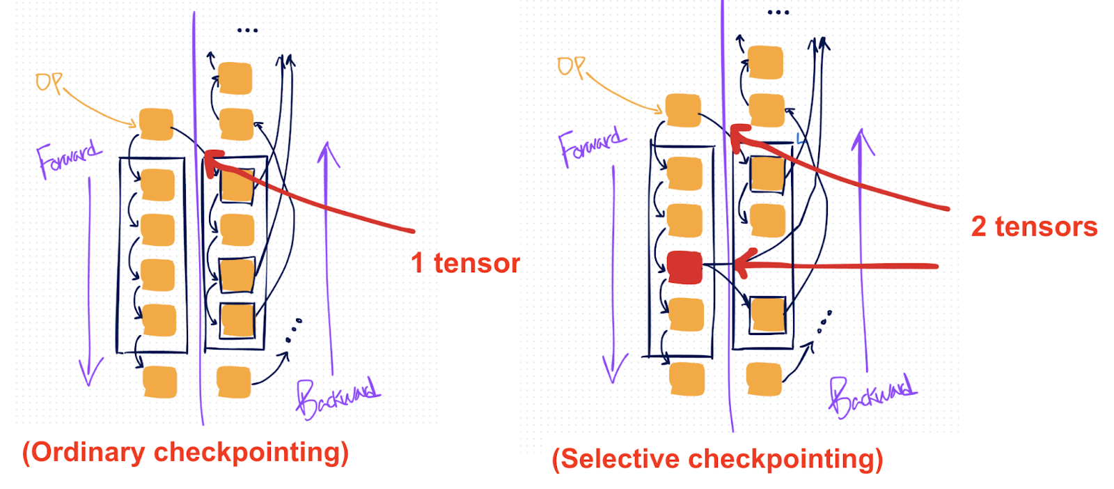
Where plain AC (left) would save a single tensor and then recompute the entire AC’d region, with SAC (right) you can selectively save specific operations (marked red) in the region, so you can avoid recomputing them.
To specify what to selectively save, you can specify a policy_fn. To illustrate the additional trade offs you can make with this, we present two simple policy functions.
Policy 1: Not recomputing matmuls:
aten = torch.ops.aten
compute_intensive_ops = [
        aten.mm,
        aten.bmm,
        aten.addmm,
]
def policy_fn(ctx, op, *args, **kwargs):
    if op in compute_intensive_ops:
        return CheckpointPolicy.MUST_SAVE
    else:
        return CheckpointPolicy.PREFER_RECOMPUTE
Policy 2: More aggressively save anything compute intensive
# torch/_functorch/partitioners.py
aten = torch.ops.aten
compute_intensive_ops = [
   aten.mm,
   aten.convolution,
   aten.convolution_backward,
   aten.bmm,
   aten.addmm,
   aten._scaled_dot_product_flash_attention,
   aten._scaled_dot_product_efficient_attention,
   aten._flash_attention_forward,
   aten._efficient_attention_forward,
   aten.upsample_bilinear2d,
   aten._scaled_mm
]
def policy_fn(ctx, op, *args, **kwargs):
    if op in compute_intensive_ops:
        return CheckpointPolicy.MUST_SAVE
    else:
        return CheckpointPolicy.PREFER_RECOMPUTE
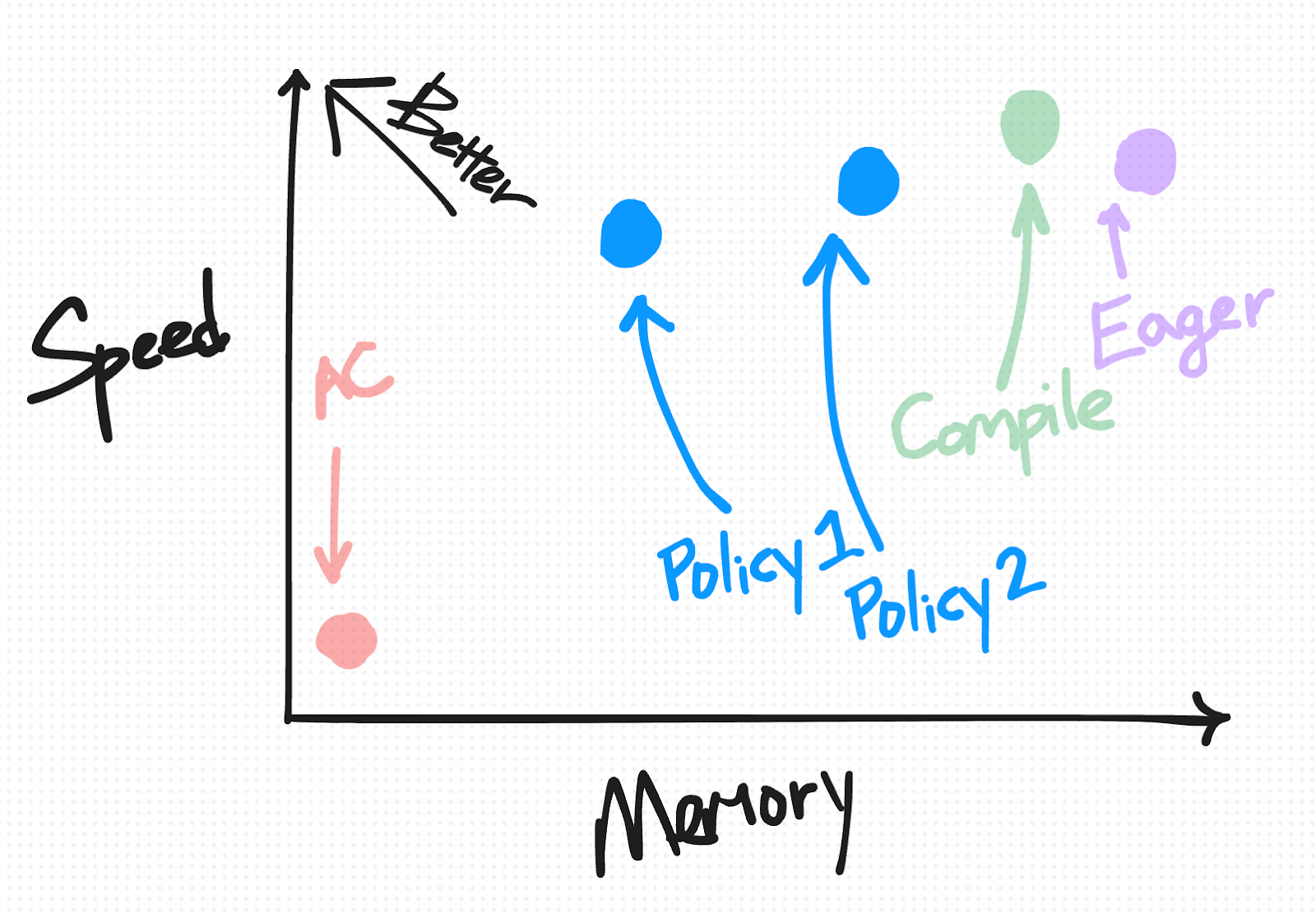
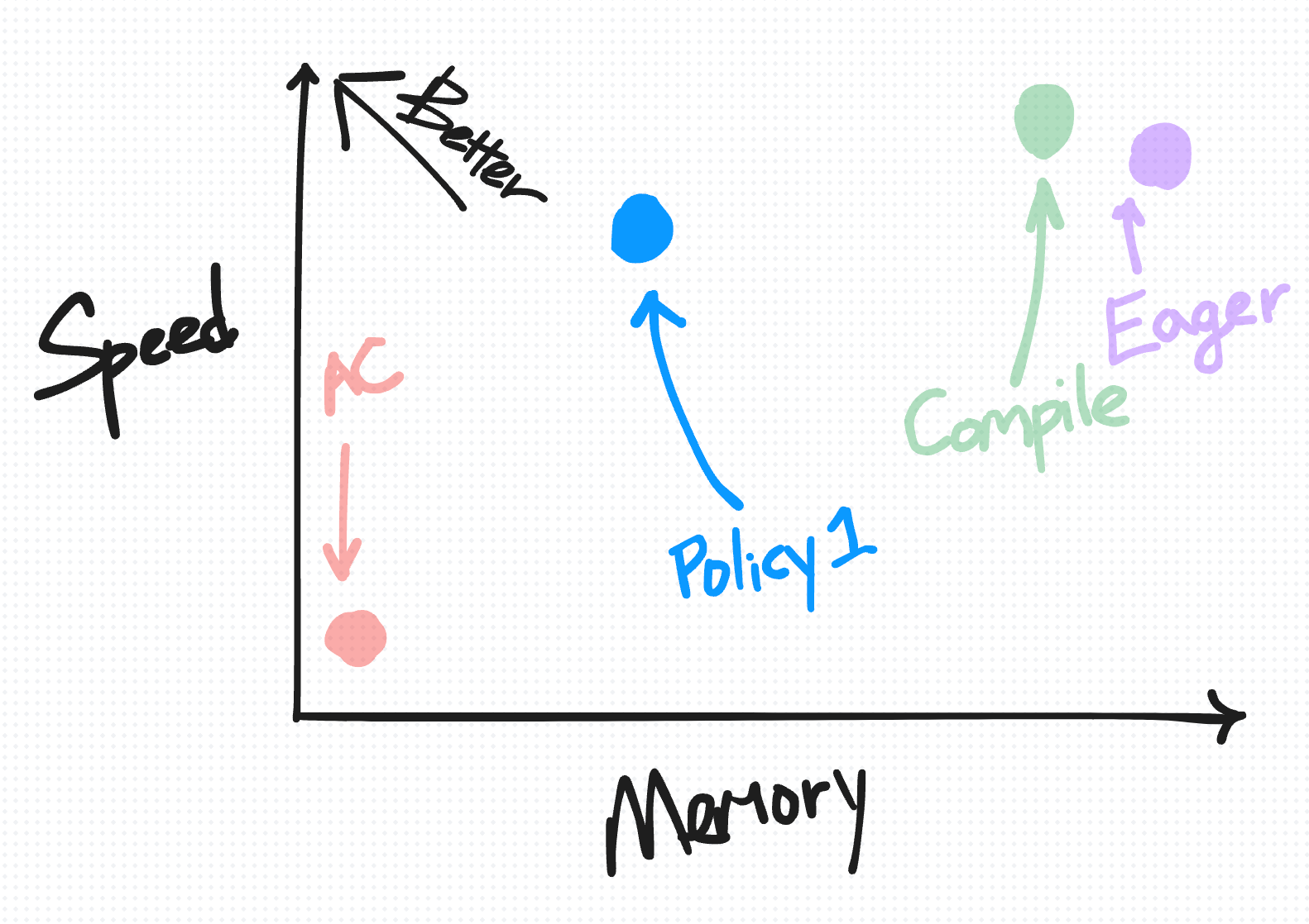
On the speed-versus-memory diagram, SAC is plotted as a range of points from closer to AC to closer to Eager, depending on your chosen policy.
Try it out! (Available in 2.5 as a prototype feature; see docs for more info + copy-pastable example)
from torch.utils.checkpoint import checkpoint, create_selective_checkpoint_contexts

# Create a policy function that returns a CheckpointPolicy
def policy_fn(ctx, op, *args, **kwargs):
    if op in ops_to_save:
        return CheckpointPolicy.MUST_SAVE
    else:
        return CheckpointPolicy.PREFER_RECOMPUTE

# Use the context_fn= arg of the existing checkpoint API
out = checkpoint(
    fn, *args,
    use_reentrant=False,
    # Fill in SAC context_fn's policy_fn with functools.partial
    context_fn=partial(create_selective_checkpoint_contexts, policy_fn),
)
(compile-only) Memory Budget API [NEW!]
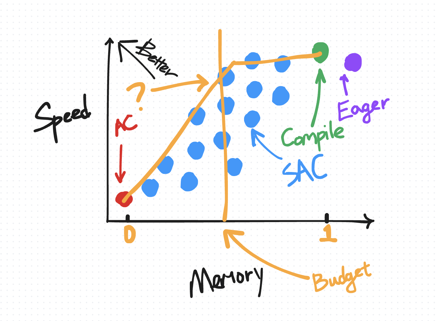
As mentioned previously, any given SAC policy can be represented as a point on a speed-memory tradeoff diagram. Not all policies are created equal, however. The “optimal” policies are the ones that fall on a pareto curve, e.g. for all policies that incur the same memory overhead, this policy is the one that minimizes the amount of required compute.
For users who are using torch.compile, we offer a memory budget API that automatically applies SAC over your compiled region with a pareto-optimal policy given a user-specified “memory budget” between 0 and 1, where a budget of 0 behaves like plain-AC and a budget of 1 behaves like default torch.compile.
Below are some real results on a transformer model:
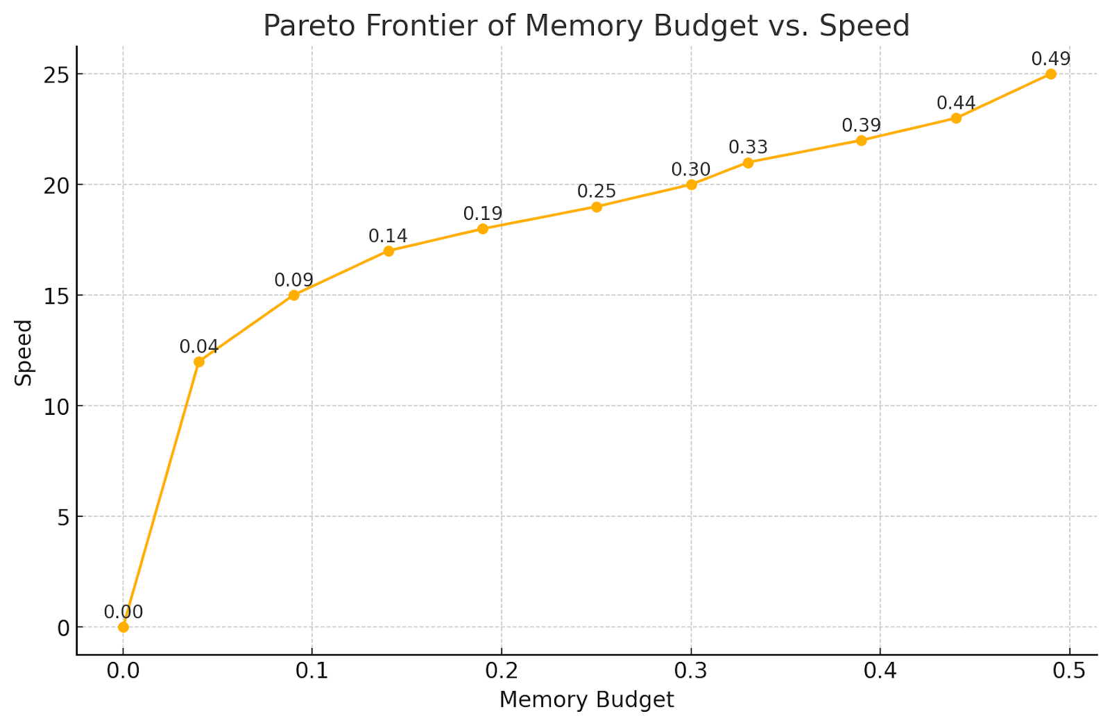
We observe a 50% memory reduction by recomputing only pointwise ops, with a steady drop-off as you recompute more and more of your matmuls. Attention is the most expensive, so you tend to want to recompute those last.
Try it out! (Available in 2.4 as an experimental feature; see this comment block for more info)
torch._dynamo.config.activation_memory_budget = 0.5

out = torch.compile(fn)(inp)
Conclusion
In summary, activation checkpointing techniques in PyTorch offer a variety of ways to balance memory and compute demands, from simple region-based checkpointing to more selective and automated methods. By choosing the option that best matches your model’s structure and resource constraints, you can achieve significant memory savings with an acceptable trade-off in compute.
Acknowledgements
We would like to thank Meta’s xformers team including Francisco Massa for working on the original version of Selective Activation Checkpoint.