Today, we are pleased to announce a new advanced CUDA feature, CUDA Graphs, has been brought to PyTorch. Modern DL frameworks have complicated software stacks that incur significant overheads associated with the submission of each operation to the GPU. When DL workloads are strong-scaled to many GPUs for performance, the time taken by each GPU operation diminishes to just a few microseconds and, in these cases, the high work submission latencies of frameworks often lead to low utilization of the GPU. As GPUs get faster and workloads are scaled to more devices, the likelihood of workloads suffering from these launch-induced stalls increases. To overcome these performance overheads, NVIDIA engineers worked with PyTorch developers to enable CUDA graph execution natively in PyTorch. This design was instrumental in scaling NVIDIA’s MLPerf workloads (implemented in PyTorch) to over 4000 GPUs in order to achieve record-breaking performance.

CUDA graphs support in PyTorch is just one more example of a long collaboration between NVIDIA and Facebook engineers. torch.cuda.amp, for example, trains with half precision while maintaining the network accuracy achieved with single precision and automatically utilizing tensor cores wherever possible. AMP delivers up to 3X higher performance than FP32 with just a few lines of code change. Similarly, NVIDIA’s Megatron-LM was trained using PyTorch on up to 3072 GPUs. In PyTorch, one of the most performant methods to scale-out GPU training is with torch.nn.parallel.DistributedDataParallel coupled with the NVIDIA Collective Communications Library (NCCL) backend.
CUDA Graphs
CUDA Graphs, which made its debut in CUDA 10, let a series of CUDA kernels to be defined and encapsulated as a single unit, i.e., a graph of operations, rather than a sequence of individually-launched operations. It provides a mechanism to launch multiple GPU operations through a single CPU operation, and hence reduces the launching overheads.
The benefits of CUDA graphs can be demonstrated with the simple example in Figure 1. On the top, a sequence of short kernels is launched one-by-one by the CPU. The CPU launching overhead creates a significant gap in between the kernels. If we replace this sequence of kernels with a CUDA graph, initially we will need to spend a little extra time on building the graph and launching the whole graph in one go on the first occasion, but subsequent executions will be very fast, as there will be very little gap between the kernels. The difference is more pronounced when the same sequence of operations is repeated many times, for example, overy many training steps. In that case, the initial costs of building and launching the graph will be amortized over the entire number of training iterations. For a more comprehensive introduction on the topic, see our blog
Getting Started with CUDA Graphs and GTC talk Effortless CUDA Graphs.
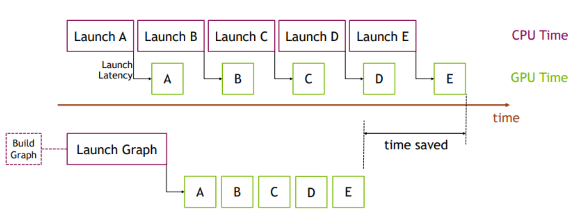
Figure 1. Benefits of using CUDA graphs
NCCL support for CUDA graphs
The previously mentioned benefits of reducing launch overheads also extend to NCCL kernel launches. NCCL enables GPU-based collective and P2P communications. With NCCL support for CUDA graphs, we can eliminate the NCCL kernel launch overhead.
Additionally, kernel launch timing can be unpredictable due to various CPU load and operating system factors. Such time skews can be harmful to the performance of NCCL collective operations. With CUDA graphs, kernels are clustered together so that performance is consistent across ranks in a distributed workload. This is especially useful in large clusters where even a single slow node can bring down overall cluster level performance.
For distributed multi-GPU workloads, NCCL is used for collective communications. If we look at training a neural network that leverages data parallelism, without NCCL support for CUDA graphs, we’ll need a separate launch for each of forward/back propagation and NCCL AllReduce. By contrast, with NCCL support for CUDA graphs, we can reduce launch overhead by lumping together the forward/backward propagation and NCCL AllReduce all in a single graph launch.
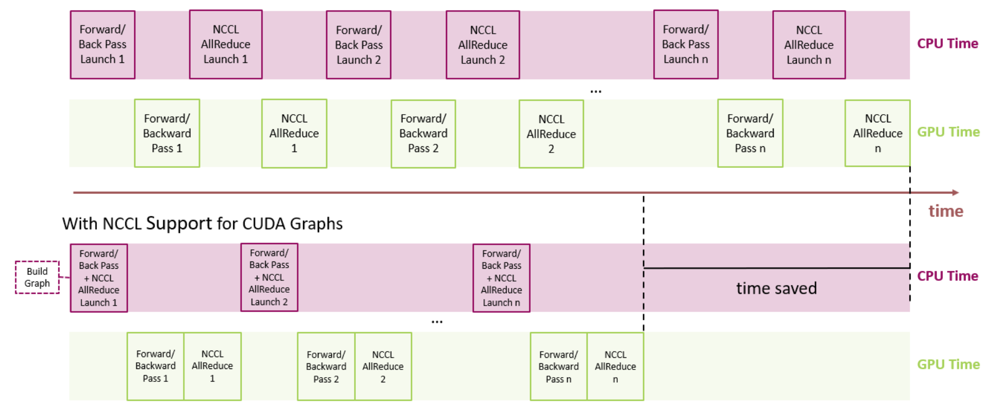
Figure 2. Looking at a typical neural network, all the kernel launches for NCCL AllReduce can be bundled into a graph to reduce overhead launch time.
PyTorch CUDA Graphs
From PyTorch v1.10, the CUDA graphs functionality is made available as a set of beta APIs.
API overview
PyTorch supports the construction of CUDA graphs using stream capture, which puts a CUDA stream in capture mode. CUDA work issued to a capturing stream doesn’t actually run on the GPU. Instead, the work is recorded in a graph. After capture, the graph can be launched to run the GPU work as many times as needed. Each replay runs the same kernels with the same arguments. For pointer arguments this means the same memory addresses are used. By filling input memory with new data (e.g., from a new batch) before each replay, you can rerun the same work on new data.
Replaying a graph sacrifices the dynamic flexibility of typical eager execution in exchange for greatly reduced CPU overhead. A graph’s arguments and kernels are fixed, so a graph replay skips all layers of argument setup and kernel dispatch, including Python, C++, and CUDA driver overheads. Under the hood, a replay submits the entire graph’s work to the GPU with a single call to cudaGraphLaunch. Kernels in a replay also execute slightly faster on the GPU, but eliding CPU overhead is the main benefit.
You should try CUDA graphs if all or part of your network is graph-safe (usually this means static shapes and static control flow, but see the other constraints) and you suspect its runtime is at least somewhat CPU-limited.
API example
PyTorch exposes graphs via a raw torch.cuda.CUDAGraphclass and two convenience wrappers, torch.cuda.graph and torch.cuda.make_graphed_callables.
torch.cuda.graph
torch.cuda.graph is a simple, versatile context manager that captures CUDA work in its context. Before capture, warm up the workload to be captured by running a few eager iterations. Warmup must occur on a side stream. Because the graph reads from and writes to the same memory addresses in every replay, you must maintain long-lived references to tensors that hold input and output data during capture. To run the graph on new input data, copy new data to the capture’s input tensor(s), replay the graph, then read the new output from the capture’s output tensor(s).
If the entire network is capture safe, one can capture and replay the whole network as in the following example.
N, D_in, H, D_out = 640, 4096, 2048, 1024
model = torch.nn.Sequential(torch.nn.Linear(D_in, H),
                            torch.nn.Dropout(p=0.2),
                            torch.nn.Linear(H, D_out),
                            torch.nn.Dropout(p=0.1)).cuda()
loss_fn = torch.nn.MSELoss()
optimizer = torch.optim.SGD(model.parameters(), lr=0.1)

# Placeholders used for capture
static_input = torch.randn(N, D_in, device='cuda')
static_target = torch.randn(N, D_out, device='cuda')

# warmup
# Uses static_input and static_target here for convenience,
# but in a real setting, because the warmup includes optimizer.step()
# you must use a few batches of real data.
s = torch.cuda.Stream()
s.wait_stream(torch.cuda.current_stream())
with torch.cuda.stream(s):
    for i in range(3):
        optimizer.zero_grad(set_to_none=True)
        y_pred = model(static_input)
        loss = loss_fn(y_pred, static_target)
        loss.backward()
        optimizer.step()
torch.cuda.current_stream().wait_stream(s)

# capture
g = torch.cuda.CUDAGraph()
# Sets grads to None before capture, so backward() will create
# .grad attributes with allocations from the graph's private pool
optimizer.zero_grad(set_to_none=True)
with torch.cuda.graph(g):
    static_y_pred = model(static_input)
    # Fills the graph's input memory with new data to compute on
    static_input.copy_(data)
    static_target.copy_(target)
    # replay() includes forward, backward, and step.
    # You don't even need to call optimizer.zero_grad() between iterations
    # because the captured backward refills static .grad tensors in place.
    g.replay()
    # Params have been updated. static_y_pred, static_loss, and .grad
    # attributes hold values from computing on this iteration's data.
If some of your network is unsafe to capture (e.g., due to dynamic control flow, dynamic shapes, CPU syncs, or essential CPU-side logic), you can run the unsafe part(s) eagerly and use torch.cuda.make_graphed_callables() to graph only the capture-safe part(s). This is demonstrated next.
torch.cuda.make_graphed_callables
make_graphed_callables accepts callables (functions or nn.Module and returns graphed versions. By default, callables returned by make_graphed_callables() are autograd-aware, and can be used in the training loop as direct replacements for the functions or nn.Module you passed. make_graphed_callables() internally creates CUDAGraph objects, runs warm up iterations, and maintains static inputs and outputs as needed. Therefore, (unlike with torch.cuda.graph) you don’t need to handle those manually.
In the following example, data-dependent dynamic control flow means the network isn’t capturable end-to-end, but make_graphed_callables() lets us capture and run graph-safe sections as graphs regardless:
N, D_in, H, D_out = 640, 4096, 2048, 1024

module1 = torch.nn.Linear(D_in, H).cuda()
module2 = torch.nn.Linear(H, D_out).cuda()
module3 = torch.nn.Linear(H, D_out).cuda()

loss_fn = torch.nn.MSELoss()
optimizer = torch.optim.SGD(chain(module1.parameters() +
                                  module2.parameters() +
                                  module3.parameters()),
                            lr=0.1)

# Sample inputs used for capture
# requires_grad state of sample inputs must match
# requires_grad state of real inputs each callable will see.
x = torch.randn(N, D_in, device='cuda')
h = torch.randn(N, H, device='cuda', requires_grad=True)

module1 = torch.cuda.make_graphed_callables(module1, (x,))
module2 = torch.cuda.make_graphed_callables(module2, (h,))
module3 = torch.cuda.make_graphed_callables(module3, (h,))

real_inputs = [torch.rand_like(x) for _ in range(10)]
real_targets = [torch.randn(N, D_out, device="cuda") for _ in range(10)]

for data, target in zip(real_inputs, real_targets):
    optimizer.zero_grad(set_to_none=True)

    tmp = module1(data)  # forward ops run as a graph

    if tmp.sum().item() > 0:
        tmp = module2(tmp)  # forward ops run as a graph
    else:
        tmp = module3(tmp)  # forward ops run as a graph

    loss = loss_fn(tmp, y)
    # module2's or module3's (whichever was chosen) backward ops,
    # as well as module1's backward ops, run as graphs
    loss.backward()
    optimizer.step()
Example use cases
MLPerf v1.0 training workloads
The PyTorch CUDA graphs functionality was instrumental in scaling NVIDIA’s MLPerf training v1.0 workloads (implemented in PyTorch) to over 4000 GPUs, setting new records across the board. We illustrate below two MLPerf workloads where the most significant gains were observed with the use of CUDA graphs, yielding up to ~1.7x speedup.
| Number of GPUs | Speedup from CUDA-graphs | |
|---|---|---|
| Mask R-CNN | 272 | 1.70× |
| BERT | 4096 | 1.12× |
Table 1. MLPerf training v1.0 performance improvement with PyTorch CUDA graph.
Mask R-CNN
Deep learning frameworks use GPUs to accelerate computations, but a significant amount of code still runs on CPU cores. CPU cores process meta-data like tensor shapes in order to prepare arguments needed to launch GPU kernels. Processing meta-data is a fixed cost while the cost of the computational work done by the GPUs is positively correlated with batch size. For large batch sizes, CPU overhead is a negligible percentage of total run time cost, but at small batch sizes CPU overhead can become larger than GPU run time. When that happens, GPUs go idle between kernel calls. This issue can be identified on an NSight timeline plot in Figure 3. The plot below shows the “backbone” portion of Mask R-CNN with per-gpu batch size of 1 before graphing. The green portion shows CPU load while the blue portion shows GPU load. In this profile we see that the CPU is maxed out at 100% load while GPU is idle most of the time, there is a lot of empty space between GPU kernels.

Figure 3: NSight timeline plot of Mask R-CNN
CUDA graphs can automatically eliminate CPU overhead when tensor shapes are static. A complete graph of all the kernel calls is captured during the first step, in subsequent steps the entire graph is launched with a single op, eliminating all the CPU overhead, as observed in Figure 4..
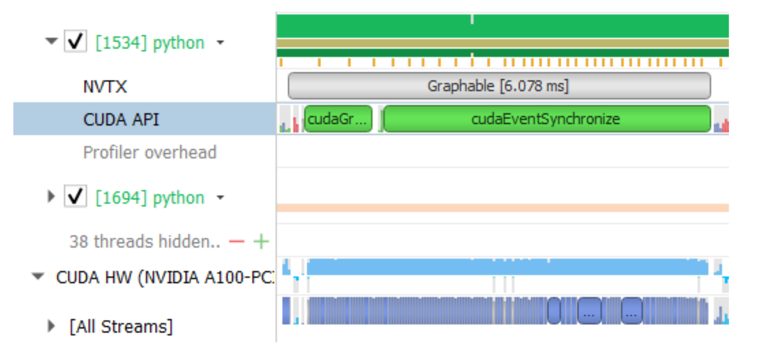
Figure 4: CUDA graphs optimization
With graphing, we see that the GPU kernels are tightly packed and GPU utilization remains high. The graphed portion now runs in 6 ms instead of 31ms, a speedup of 5x. We did not graph the entire model, mostly just the resnet backbone, which resulted in an overall speedup of ~1.7x.
In order to increase the scope of the graph, we made some changes in the software stack to eliminate some of the CPU-GPU synchronization points. In MLPerf v1.0, this work included changing the implementation of torch.randperm function to use CUB instead of Thrust because the latter is a synchronous C++ template library. These improvements are available in the latest NGC container.
BERT
Similarly, by graph capturing the model, we eliminate CPU overhead and accompanying synchronization overhead. CUDA graphs implementation results in a 1.12x performance boost for our max-scale BERT configuration. To maximize the benefits from CUDA graphs, it is important to keep the scope of the graph as large as possible. To achieve this, we modified the model script to remove CPU-GPU synchronizations during the execution such that the full model can be graph captured. Furthermore, we also made sure that the tensor sizes during the execution are static within the scope of the graph. For instance, in BERT, only a specific subset of total tokens contribute to loss function, determined by a pre-generated mask tensor. Extracting the indices of valid tokens from this mask, and using these indices to gather the tokens that contribute to the loss, results in a tensor with a dynamic shape, i.e. with shape that is not constant across iterations. In order to make sure tensor sizes are static, instead of using the dynamic-shape tensors in the loss computation, we used static shape tensors where a mask is used to indicate which elements are valid. As a result, all tensor shapes are static. Dynamic shapes also require CPU-GPU synchronization since it has to involve the framework’s memory management on the CPU side. With static-only shapes, no CPU-GPU synchronizations are necessary. This is shown in Figure 5.

Figure 5. By using a fixed size tensor and a boolean mask as described in the text, we are able to eliminate CPU synchronizations needed for dynamic sized tensors
CUDA graphs in NVIDIA DL examples collection
Single GPU use cases can also benefit from using CUDA Graphs. This is particularly true for workloads launching many short kernels with small batches. A good example is training and inference for recommender systems. Below we present preliminary benchmark results for NVIDIA’s implementation of the Deep Learning Recommendation Model (DLRM) from our Deep Learning Examples collection. Using CUDA graphs for this workload provides significant speedups for both training and inference. The effect is particularly visible when using very small batch sizes, where CPU overheads are more pronounced.
CUDA graphs are being actively integrated into other PyTorch NGC model scripts and the NVIDIA Github deep learning examples. Stay tuned for more examples on how to use it.
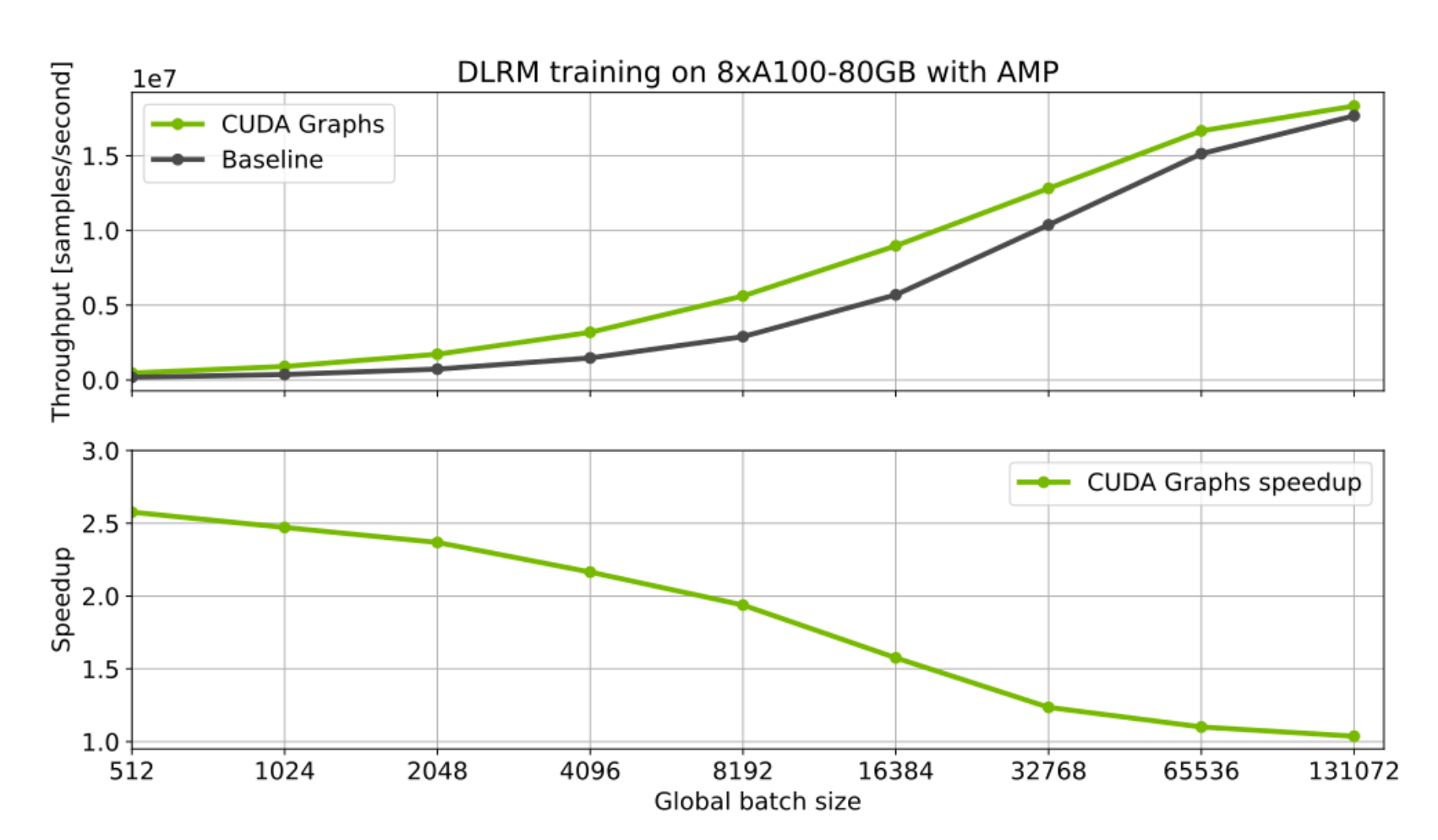
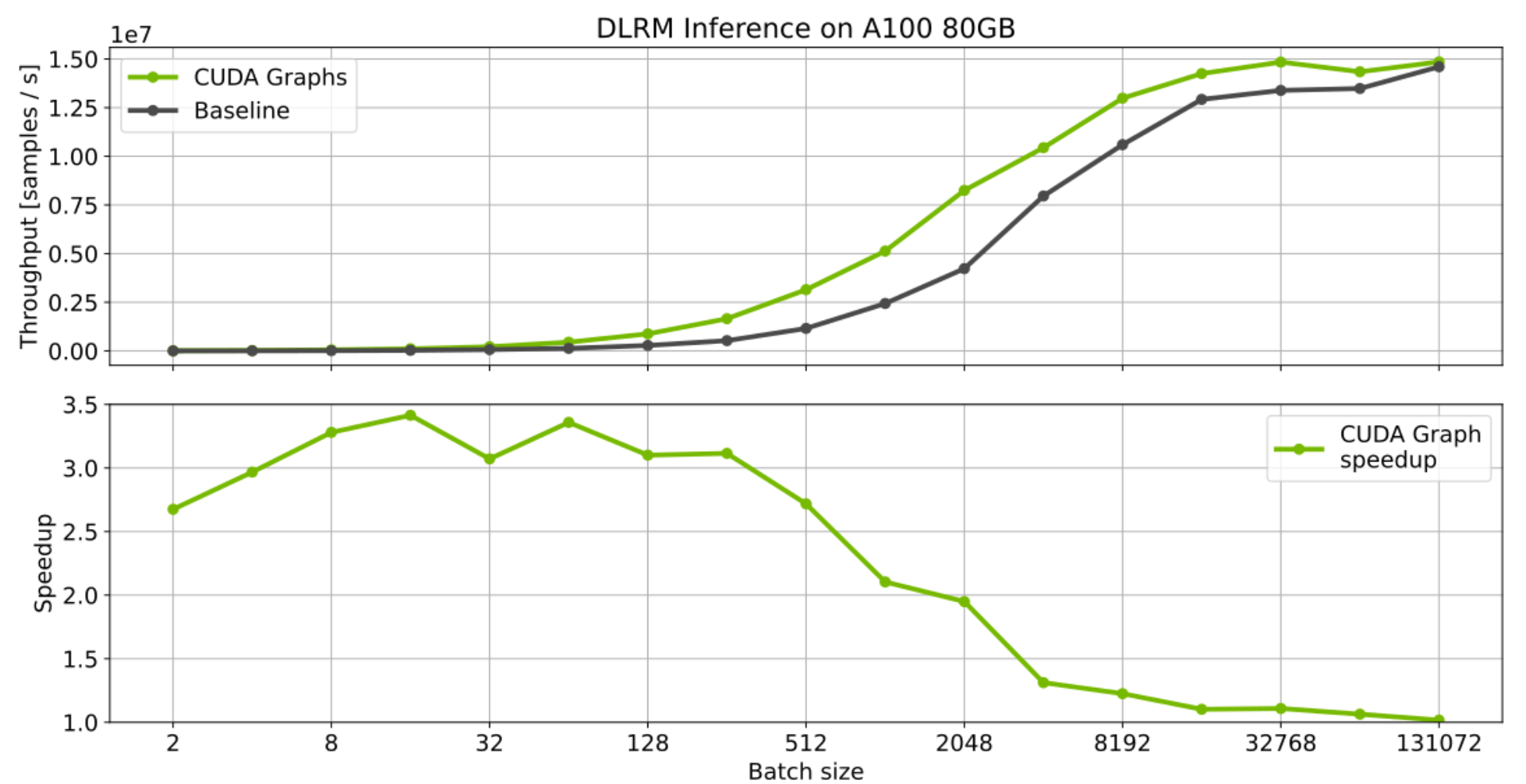
Figure 6: CUDA graphs optimization for the DLRM model.
Call to action: CUDA Graphs in PyTorch v1.10
CUDA graphs can provide substantial benefits for workloads that comprise many small GPU kernels and hence bogged down by CPU launch overheads. This has been demonstrated in our MLPerf efforts, optimizing PyTorch models. Many of these optimizations, including CUDA graphs, have or will eventually be integrated into our PyTorch NGC model scripts collection and the NVIDIA Github deep learning examples. For now, check out our open-source MLPerf training v1.0 implementation which could serve as a good starting point to see CUDA graph in action. Alternatively, try the PyTorch CUDA graphs API on your own workloads.
We thank many NVIDIAN’s and Facebook engineers for their discussions and suggestions:
Karthik Mandakolathur US,
Tomasz Grel,
PLJoey Conway,
Arslan Zulfiqar US
Authors bios
Vinh Nguyen
DL Engineer, NVIDIA
Vinh is a Deep learning engineer and data scientist, having published more than 50 scientific articles attracting more than 2500 citations. At NVIDIA, his work spans a wide range of deep learning and AI applications, including speech, language and vision processing, and recommender systems.
Michael Carilli
Senior Developer Technology Engineer, NVIDIA
Michael worked at the Air Force Research Laboratory optimizing CFD code for modern parallel architectures. He holds a PhD in computational physics from the University of California, Santa Barbara. A member of the PyTorch team, he focuses on making GPU training fast, numerically stable, and easy(er) for internal teams, external customers, and Pytorch community users.
Sukru Burc Eryilmaz
Senior Architect in Dev Arch, NVIDIA
Sukru received his PhD from Stanford University, and B.S from Bilkent University. He currently works on improving the end-to-end performance of neural network training both at single-node scale and supercomputer scale.
Vartika Singh
Tech Partner Lead for DL Frameworks and Libraries, NVIDIA
Vartika has led teams working in confluence of cloud and distributed computing, scaling and AI, influencing the design and strategy of major corporations. She currently works with the major frameworks and compiler organizations and developers within and outside NVIDIA, to help the design to work efficiently and optimally on NVIDIA hardware.
Michelle Lin
Product Intern, NVIDIA
Michelle is currently pursuing an undergraduate degree in Computer Science and Business Administration at UC Berkeley. She is currently managing execution of projects such as conducting market research and creating marketing assets for Magnum IO.
Natalia Gimelshein
Applied Research Scientist, Facebook
Natalia Gimelshein worked on GPU performance optimization for deep learning workloads at NVIDIA and Facebook. She is currently a member of the PyTorch core team, working with partners to seamlessly support new software and hardware features.
Alban Desmaison
Research Engineer, Facebook
Alban studied engineering and did a PhD in Machine Learning and Optimization, during which he was an OSS contributor to PyTorch prior to joining Facebook. His main responsibilities are maintaining some core library and features (autograd, optim, nn) and working on making PyTorch better in general.
Edward Yang
Research Engineer, Facebook
Edward studied CS at MIT and then Stanford before starting at Facebook. He is a part of the PyTorch core team and is one of the leading contributors to PyTorch.
