Editor’s note: This is a guest post written by Michael Malahe, Head of Data at Aerobotics, a South African startup that builds AI-driven tools for agriculture.
Aerobotics is an agri-tech company operating in 18 countries around the world, based out of Cape Town, South Africa. Our mission is to provide intelligent tools to feed the world. We aim to achieve this by providing farmers with actionable data and insights on our platform, Aeroview, so that they can make the necessary interventions at the right time in the growing season. Our predominant data source is aerial drone imagery: capturing visual and multispectral images of trees and fruit in an orchard.
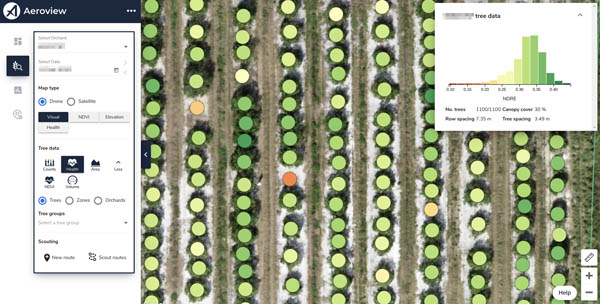
In this post we look at how we use Amazon SageMaker and TensorFlow to improve our Tree Insights product, which provides per-tree measurements of important quantities like canopy area and health, and provides the locations of dead and missing trees. Farmers use this information to make precise interventions like fixing irrigation lines, applying fertilizers at variable rates, and ordering replacement trees. The following is an image of the tool that farmers use to understand the health of their trees and make some of these decisions.
To provide this information to make these decisions, we first must accurately assign each foreground pixel to a single unique tree. For this instance segmentation task, it’s important that we’re as accurate as possible, so we use a machine learning (ML) model that’s been effective in large-scale benchmarks. The model is a variant of Mask R-CNN, which pairs a convolutional neural network (CNN) for feature extraction with several additional components for detection, classification, and segmentation. In the following image, we show some typical outputs, where the pixels belong to a given tree are outlined by a contour.
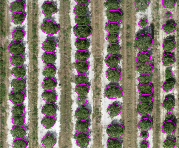
Glancing at the outputs, you might think that the problem is solved.
The challenge
The main challenge with analyzing and modeling agricultural data is that it’s highly varied across a number of dimensions.
The following image illustrates some extremes of the variation in the size of trees and the extent to which they can be unambiguously separated.
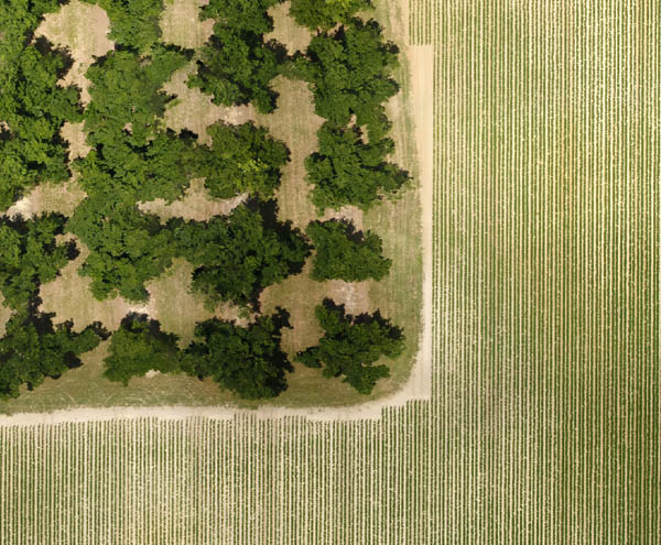
In the grove of pecan trees, we have one of the largest trees in our database, with an area of 654 m2 (a little over a minute to walk around at a typical speed). The vines to the right of the grove measure 50 cm across (the size of a typical potted plant). Our models need to be tolerant to these variations to provide accurate segmentations regardless of the scale.
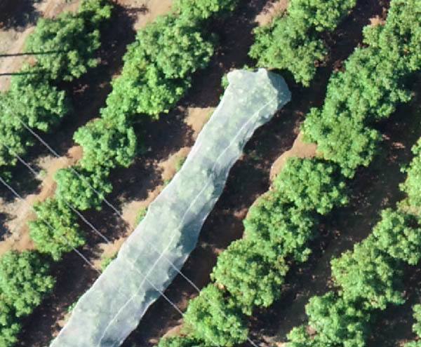
An additional challenge is that the sources of variation aren’t static. Farmers are highly innovative, and best practices can change significantly over time. One example is ultra-high-density planting for apples, where trees are planted as close as a foot apart. Another is the adoption of protective netting, which obscures aerial imagery, as in the following image.
In this domain with broad and shifting variations, we need to maintain accurate models to provide our clients with reliable insights. Models should improve with every challenging new sample we encounter, and we should deploy them with confidence.
In our initial approach to this challenge, we simply trained on all the data we had. As we scaled, however, we quickly got to the point where training on all our data became infeasible, and the cost of doing so became an impediment to experimentation.
The solution
Although we have variation in the edge cases, we recognized that there was a lot of redundancy in our standard cases. Our goal was to get to a point where our models are trained on only the most salient data, and can converge without needing to see every sample. Our approach to achieving this was first to create an environment where it’s simple to experiment with different approaches to dataset construction and sampling. The following diagram shows our overall workflow for the data preprocessing that enables this.

The outcome is that training samples are available as individual files in Amazon Simple Storage Service (Amazon S3), which is only sensible to do with bulky data like multispectral imagery, with references and rich metadata stored in Amazon Redshift tables. This makes it trivial to construct datasets with a single query, and makes it possible to fetch individual samples with arbitrary access patterns at train time. We use UNLOAD to create an immutable dataset in Amazon S3, and we create a reference to the file in our Amazon Relational Database Service (Amazon RDS) database, which we use for training provenance and evaluation result tracking. See the following code:
UNLOAD ('[subset_query]')
TO '[s3://path/to/dataset]'
IAM_ROLE '[redshift_write_to_s3_role]'
FORMAT PARQUET
The ease of querying the tile metadata allowed us to rapidly create and test subsets of our data, and eventually we were able to train to convergence after seeing only 1.1 million samples of a total 3.1 million. This sub-epoch convergence has been very beneficial in bringing down our compute costs, and we got a better understanding of our data along the way.
The second step we took in reducing our training costs was to optimize our compute. We used the TensorFlow profiler heavily throughout this step:
import tensorflow as tf
tf.profiler.experimental.ProfilerOptions(host_tracer_level=2,  python_tracer_level=1,device_tracer_level=1)
tf.profiler.experimental.start("[log_dir]")
[train model]
tf.profiler.experimental.stop()
For training, we use Amazon SageMaker with P3 instances provisioned by Amazon Elastic Compute Cloud (Amazon EC2), and initially we found that the NVIDIA Tesla V100 GPUs in the instances were bottlenecked by CPU compute in the input pipeline. The overall pattern for alleviating the bottleneck was to shift as much of the compute from native Python code to TensorFlow operations as possible to ensure efficient thread parallelism. The largest benefit was switching to tf.io for data fetching and deserialization, which improved throughput by 41%. See the following code:
serialised_example = tf.io.decode_compressed(tf.io.gfile.GFile(fname, 'rb').read(), compression_type='GZIP')
example = tf.train.Example.FromString(serialised_example.numpy())
A bonus feature with this approach was that switching between local files and Amazon S3 storage required no code changes due to the file object abstraction provided by GFile.
We found that the last remaining bottleneck came from the default TensorFlow CPU parallelism settings, which we optimized using a SageMaker hyperparameter tuning job (see the following example config).
With the CPU bottleneck removed, we moved to GPU optimization, and made the most of the V100’s Tensor Cores by using mixed precision training:
from tensorflow.keras.mixed_precision import experimental as mixed_precision
policy = mixed_precision.Policy('mixed_float16')
mixed_precision.set_policy(policy)
The mixed precision guide is a solid reference, but the change to using mixed precision still requires some close attention to ensure that the operations happening in half precision are not ill-conditioned or prone to underflow. Some specific cases that were critical were terminal activations and custom regularization terms. See the following code:
import tensorflow as tf
...
y_pred = tf.keras.layers.Activation('sigmoid', dtype=tf.float32)(x)
loss = binary_crossentropy(tf.cast(y_true, tf.float32), tf.cast(y_pred, tf.float32), from_logits=True)
...
model.add_loss(lambda: tf.keras.regularizers.l2()(tf.cast(w, tf.float32)))
After implementing this, we measured the following benchmark results for a single V100.
| Precision | CPU parallelism | Batch size | Samples per second |
| single | default | 8 | 9.8 |
| mixed | default | 16 | 19.3 |
| mixed | optimized | 16 | 22.4 |
The impact of switching to mixed precision was that training speed roughly doubled, and the impact of using the optimal CPU parallelism settings discovered by SageMaker was an additional 16% increase.
Implementing these initiatives as we grew resulted in reducing the cost of training a model from $122 to $68, while our dataset grew from 228 thousand samples to 3.1 million, amounting to a 24 times reduction in cost per sample.
Conclusion
This reduction in training time and cost has meant that we can quickly and cheaply adapt to changes in our data distribution. We often encounter new cases that are confounding even for humans, such as the following image.
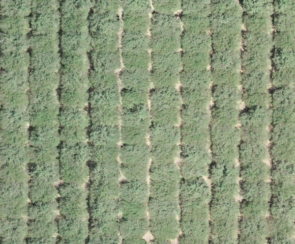
However, they quickly become standard cases for our models, as shown in the following image.
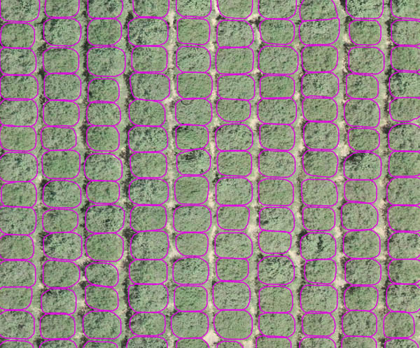
We aim to continue making training faster by using more devices, and making it more efficient by leveraging SageMaker managed Spot Instances. We also aim to make the training loop tighter by serving SageMaker models that are capable of online learning, so that improved models are available in near-real time. With these in place, we should be well equipped to handle all the variation that agriculture can throw at us. To learn more about Amazon SageMaker, visit the product page.
The content and opinions in this post are those of the third-party author and AWS is not responsible for the content or accuracy of this post.
About the Author
Michael Malahe is the Head of Data at Aerobotics, a South African startup that builds AI-driven tools for agriculture.
