Google Ads infrastructure runs on an internal data warehouse called Napa. Billions of reporting queries, which power critical dashboards used by advertising clients to measure campaign performance, run on tables stored in Napa. These tables contain records of ads performance that are keyed using particular customers and the campaign identifiers with which they are associated. Keys are tokens that are used both to associate an ads record with a particular client and campaign (e.g., customer_id, campaign_id) and for efficient retrieval. A record contains dozens of keys, so clients use reporting queries to specify keys needed to filter the data to understand ads performance (e.g., by region, device and metrics such as clicks, etc.). What makes this problem challenging is that the data is skewed since queries require varying levels of effort to be answered and have stringent latency expectations. Specifically, some queries require the use of millions of records while others are answered with just a few.
To this end, in “Progressive Partitioning for Parallelized Query Execution in Napa”, presented at VLDB 2023, we describe how the Napa data warehouse determines the amount of machine resources needed to answer reporting queries while meeting strict latency targets. We introduce a new progressive query partitioning algorithm that can parallelize query execution in the presence of complex data skews to perform consistently well in a matter of a few milliseconds. Finally, we demonstrate how Napa allows Google Ads infrastructure to serve billions of queries every day.
Query processing challenges
When a client inputs a reporting query, the main challenge is to determine how to parallelize the query effectively. Napa’s parallelization technique breaks up the query into even sections that are equally distributed across available machines, which then process these in parallel to significantly reduce query latency. This is done by estimating the number of records associated with a specified key, and assigning more or less equal amounts of work to machines. However, this estimation is not perfect since reviewing all records would require the same effort as answering the query. A machine that processes significantly more than others would result in run-time skews and poor performance. Each machine also needs to have sufficient work since needless parallelism leads to underutilized infrastructure. Finally, parallelization has to be a per query decision that must be executed near-perfectly billions of times, or the query may miss the stringent latency requirements.
The reporting query example below extracts the records denoted by keys (i.e., customer_id and campaign_id) and then computes an aggregate (i.e., SUM(cost)) from an advertiser table. In this example the number of records is too large to process on a single machine, so Napa needs to use a subsequent key (e.g., adgroup_id) to further break up the collection of records so that equal distribution of work is achieved. It is important to note that at petabyte scale, the size of the data statistics needed for parallelization may be several terabytes. This means that the problem is not just about collecting enormous amounts of metadata, but also how it is managed.
        SELECT customer_id, campaign_id, SUM(cost)
             FROM advertiser_table
             WHERE customer_id in (1, 7, ..., x )
             AND campaign_id in (10, 20, ..., y)
             GROUP BY customer_id, campaign_id;
This reporting query example extracts records denoted by keys (i.e., customer_id and campaign_id) and then computes an aggregate (i.e., SUM(cost)) from an advertiser table. The query effort is determined by the keys’ included in the query. Keys belonging to clients with larger campaigns may touch millions of records since the data volume directly correlates with the size of the ads campaign. This disparity of matching records based on keys reflects the skewness in data, which makes query processing a challenging problem. |
An effective solution minimizes the amount of metadata needed, focuses effort primarily on the skewed part of the key space to partition data efficiently, and works well within the allotted time. For example, if the query latency is a few hundred milliseconds, partitioning should take no longer than tens of milliseconds. Finally, a parallelization process should determine when it’s reached the best possible partitioning that considers query latency expectations. To this end, we have developed a progressive partitioning algorithm that we describe later in this article.
Managing the data deluge
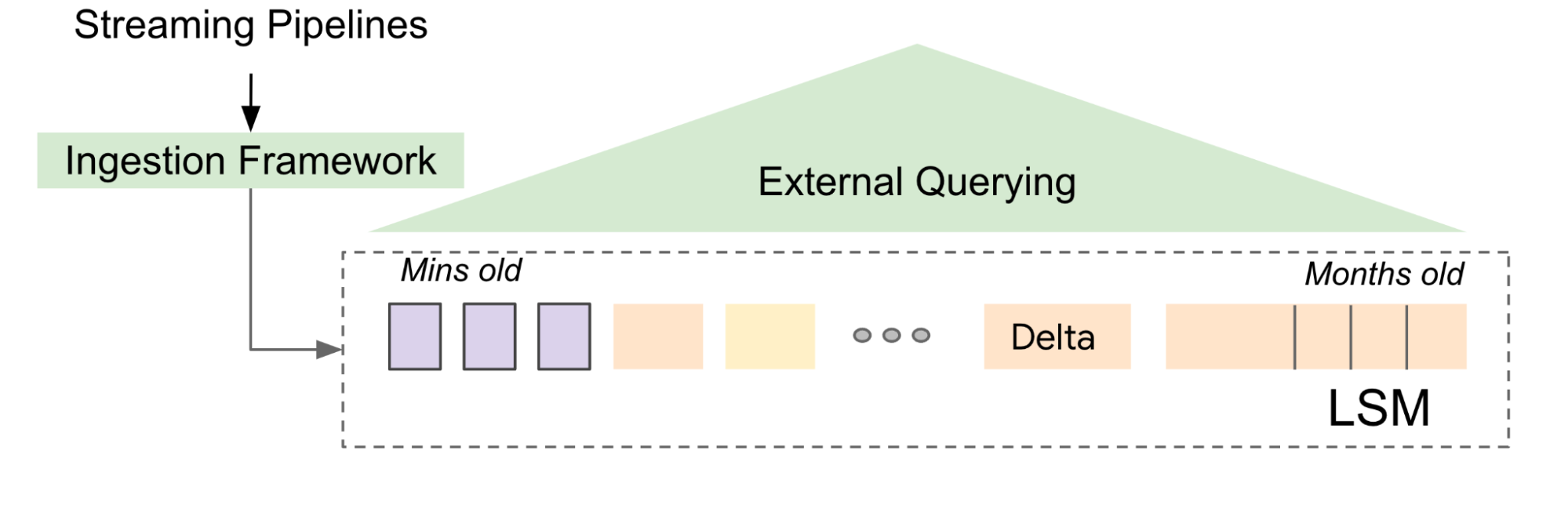
Tables in Napa are constantly updated, so we use log-structured merge forests (LSM tree) to organize the deluge of table updates. LSM is a forest of sorted data that is temporally organized with a B-tree index to support efficient key lookup queries. B-trees store summary information of the sub-trees in a hierarchical manner. Each B-tree node records the number of entries present in each subtree, which aids in the parallelization of queries. LSM allows us to decouple the process of updating the tables from the mechanics of query serving in the sense that live queries go against a different version of the data, which is atomically updated once the next batch of ingest (called delta) has been fully prepared for querying.
 |
The partitioning problem
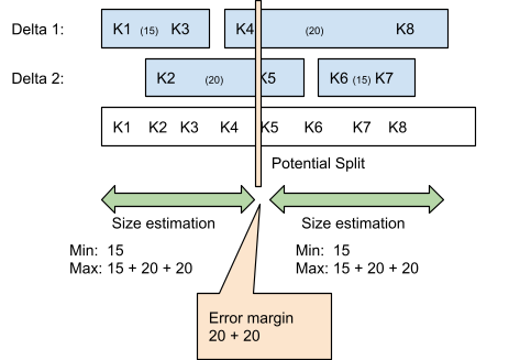
The data partitioning problem in our context is that we have a massively large table that is represented as an LSM tree. In the figure below, Delta 1 and 2 each have their own B-tree, and together represent 70 records. Napa breaks the records into two pieces, and assigns each piece to a different machine. The problem becomes a partitioning problem of a forest of trees and requires a tree-traversal algorithm that can quickly split the trees into two equal parts.
To avoid visiting all the nodes of the tree, we introduce the concept of “good enough” partitioning. As we begin cutting and partitioning the tree into two parts, we maintain an estimate of how bad our current answer would be if we terminated the partitioning process at that instant. This is the yardstick of how close we are to the answer and is represented below by a total error margin of 40 (at this point of execution, the two pieces are expected to be between 15 and 35 records in size, the uncertainty adds up to 40). Each subsequent traversal step reduces the error estimate, and if the two pieces are approximately equal, it stops the partitioning process. This process continues until the desired error margin is reached, at which time we are guaranteed that the two pieces are more or less equal.
 |
Progressive partitioning algorithm
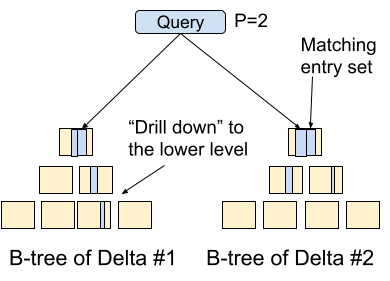
Progressive partitioning encapsulates the notion of “good enough” in that it makes a series of moves to reduce the error estimate. The input is a set of B-trees and the goal is to cut the trees into pieces of more or less equal size. The algorithm traverses one of the trees (“drill down” in the figure) which results in a reduction of the error estimate. The algorithm is guided by statistics that are stored with each node of the tree so that it makes an informed set of moves at each step. The challenge here is to decide how to direct effort in the best possible way so that the error bound reduces quickly in the fewest possible steps. Progressive partitioning is conducive for our use-case since the longer the algorithm runs, the more equal the pieces become. It also means that if the algorithm is stopped at any point, one still gets good partitioning, where the quality corresponds to the time spent.
 |
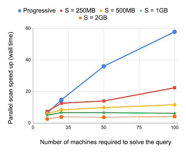
Prior work in this space uses a sampled table to drive the partitioning process, while the Napa approach uses a B-tree. As mentioned earlier, even just a sample from a petabyte table can be massive. A tree-based partitioning method can achieve partitioning much more efficiently than a sample-based approach, which does not use a tree organization of the sampled records. We compare progressive partitioning with an alternative approach, where sampling of the table at various resolutions (e.g., 1 record sample every 250 MB and so on) aids the partitioning of the query. Experimental results show the relative speedup from progressive partitioning for queries requiring varying numbers of machines. These results demonstrate that progressive partitioning is much faster than existing approaches and the speedup increases as the size of the query increases.
 |
Conclusion
Napa’s progressive partitioning algorithm efficiently optimizes database queries, enabling Google Ads to serve client reporting queries billions of times each day. We note that tree traversal is a common technique that students in introductory computer science courses use, yet it also serves a critical use-case at Google. We hope that this article will inspire our readers, as it demonstrates how simple techniques and carefully designed data structures can be remarkably potent if used well. Check out the paper and a recent talk describing Napa to learn more.
Acknowledgements
This blog post describes a collaborative effort between Junichi Tatemura, Tao Zou, Jagan Sankaranarayanan, Yanlai Huang, Jim Chen, Yupu Zhang, Kevin Lai, Hao Zhang, Gokul Nath Babu Manoharan, Goetz Graefe, Divyakant Agrawal, Brad Adelberg, Shilpa Kolhar and Indrajit Roy.
