In this tutorial, we will walk through the entire machine learning (ML) life-cycle and show you how to architect and build an ML use case end to end using Amazon SageMaker. Amazon SageMaker provides a rich set of capabilities that enable data scientists, machine learning engineers, and developers to prepare, build, train, and deploy ML models rapidly and with ease. For our use case, we have chosen an automobile claims fraud detection example.
We will initially provide an architectural walkthrough of the various portions of the ML lifecycle and then point to the code that builds each section of the lifecycle on SageMaker.
To get started, data scientists use an experimental process to explore various data preparation tasks, in some cases engineering features, and eventually settle on a standard way of doing so. Then they embark on a more repeatable and scalable process of automating stages of this process, until the model provides the necessary levels of performance (such as accuracy, F1 score, and precision). Then they package this process in a repeatable, automated, and scalable ML pipeline.
The following diagram illustrates the manual investigative and the automated operational workflows.
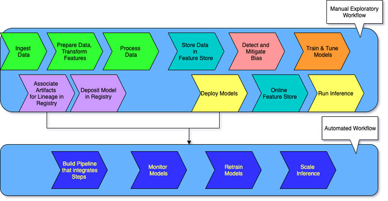
New capabilities required for new tasks in the ML lifecycle
At a high level, the ML lifecycle looks like the following diagram.
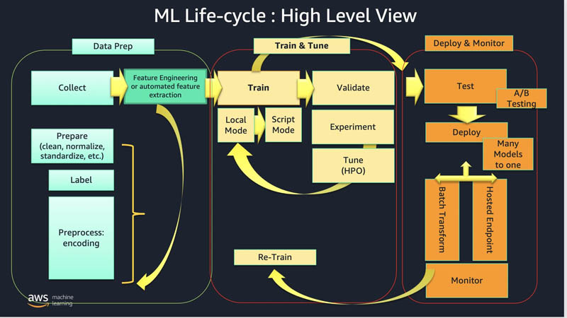
The general phases of the ML lifecycle are data preparation, train and tune, and deploy and monitor, with inference being when we actually serve the model up with new data for inference.
As ML evolves and matures in the industry, we see an increased need for activities that support various facets of scaling of ML tasks and artifacts; making the artifacts that are the outputs of each task consistently standardized, more accessible, more transparent, and therefore more governable. In addition, each of these activities needs to scale from an exploratory activity to a consistent, automated and scalable activity via automated pipelines.
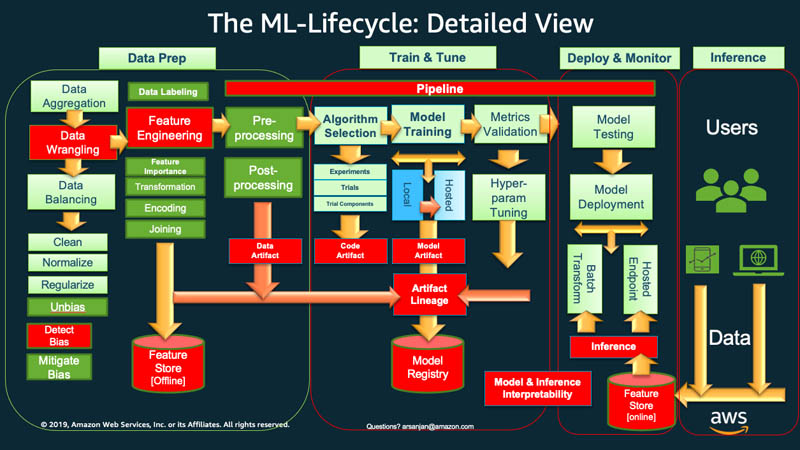
In the detailed preceding ML Lifecycle diagram, the red boxes represent comparatively newer concepts and tasks that are now deemed important to include in, and run in a scalable, operational, and production-oriented (vs. research-oriented) environment.
These newer lifecycle tasks and their corresponding Amazon SageMaker capabilities include the following:
- Data wrangling – We use SageMaker Data Wrangler for cleaning, normalizing, transforming and encoding data, as well as joining datasets. The output of SageMaker Data Wrangler is data transformation code that works with SageMaker Processing, SageMaker Pipelines, SageMaker Feature Store, or with Pandas in a plain Python script. Feature engineering can now be done faster and easier, with SageMaker Data Wrangler where we have a GUI-based environment and can generate code that can be used for the subsequent phases of the ML lifecycle.
- Detecting bias – With SageMaker Clarify, in the data prep or training phases, we can detect pre-training (data bias) and post-training bias (model bias). At the inference phase, SageMaker Clarify gives us the ability to provide interpretability and explainability of the predictions by providing insight into which factors were most influential in coming up with the prediction.
- Feature Store (offline) – After we complete our feature engineering, encoding, and transformations, we can standardize features offline in SageMaker Feature Store, to be used as input features for training models.
SageMaker Feature Store allows you to create offline feature groups that keep all the historical data and can be used as inputs to training.
Note that Features can be ingested from a feature processing pipeline into the online feature store and will then get replicated to the offline store. The offline store could be used to run batch inference as well. Thus, the online feature store can also be used as input for training. - Artifact lineage: We can use SageMaker ML Lineage Tracking to associate all the artifacts (such as data, models, and parameters) with a trained model to produce metadata that is stored in a model registry. In addition, tracking human in the loop actions such as model approvals and deployments further facilitates the process of ML governance.
- Model Registry: The SageMaker Model Registry stores the metadata around all the artifacts that you include in the process of creating your models, along with the trained models themselves in a model registry. Later, we can use human approval to note that the model is ready for production. This feeds into the next phase of deploy and monitor.
- Inference and Feature Store (online): SageMaker Feature Store provides for low latency (up to single digit milliseconds) and high throughput reads for serving our model with new incoming data.
- Pipelines: After we experiment and decide on the various options in the lifecycle (such as which transforms to apply to our features, determine imbalance or bias in the data, which algorithms to choose to train with, or which hyperparameters are giving us the best performance metrics), we can automate the various tasks across the lifecycle using SageMaker Pipelines.
This lets us streamline the otherwise cumbersome manual processes into an automated ML pipeline. To build this pipeline, we will prepare some data (customers and claims) by ingesting the data into SageMaker Data Wrangler and apply various transformations in SageMaker Data Wrangler within SageMaker Studio. SageMaker Data Wrangler creates .flow files. We will use these transformation definitions as a starting point for our automated pipeline and go through the ML Lifecycle all the way to deploying the model to a SageMaker Hosted Endpoint. Note that some use cases may require one, larger, end-to-end pipeline, that does everything. Other use cases may require multiple pipelines, such as the following:
-
- A pipeline for all data prep steps.
- A pipeline for training, tuning, lineage, and depositing into the model registry (which we show in the code associated with this post).
- Possibly another pipeline for specific inference scenarios (such as real time vs. batch).
- A pipeline for triggering retraining by using SageMaker Model Monitor to detect model drift or data drift and trigger retraining using, for example, an AWS Lambda
Use case: Fraud detection for auto insurance claims
In this post, we use an auto insurance claim fraud detection use case to demonstrate how you can easily use Amazon SageMaker to predict the probability that an incoming auto claim may be fraudulent.
We dive into the implementation details in these six notebooks, where we demonstrate how you can enhance your effectiveness as a data scientist and ML engineer by using the new Amazon SageMaker services and features (pictured in red in the preceding figure) to solve problems at each stage of the ML lifecycle.
Technical solution overview
Let’s take a look at the services used in the ML lifecycle for implementing our fraud detection use case. Each section has an accompanying notebook on GitHub that you can follow as you read through the explanations in this post.
Wrangling and preprocessing the dataset
We use two synthetic datasets, consisting of customers and claims that we have synthetically generated. We use SageMaker Data Wrangler to ingest, analyze, prepare, and transform each dataset. You can do this in the GUI-based feature available in SageMaker Studio.
Second, we use SageMaker Data Wrangler to export the transformed data as two CSV files that can be picked up in an Amazon Simple Storage Service (Amazon S3) bucket by SageMaker Processing, in order to conduct scalable data preparation and preprocessing.
Storing the features
After SageMaker Processing applies the transformations defined in SageMaker Data Wrangler, we store the normalized features in an offline feature store so the features can be shared and reused consistently across an organization among collaborating data scientists. This standardization is often key to creating a normalized, reusable set of features that can be created, shared, and managed as input into training ML models. You can use this feature consistency across the ML maturity spectrum, whether you are a startup or an advanced organization with a ML Center of Excellence.
Assessing and Mitigating bias, training and tuning
The issues relating to bias detection and fairness in AI have taken a prominent role in ML. Data bias is often inadvertently injected during the data labeling and collection process, and may often be overlooked in the significance of its impact on training a model. SageMaker Clarify is a fully-managed toolkit to identify potential bias within a training dataset or model, explain individual inference results, aggregate these explanations for an entire dataset, integrate with built-in monitoring capabilities to assess production performance, and provide these capabilities across modeling frameworks.
You can use SageMaker Clarify to assess various types of bias. For example, assessing pre-training bias (data) can focus on determining if class imbalance or a variety of other factors are beyond a threshold and therefore may bias the model we seek to train. SageMaker Clarify helps improve your ML models by detecting potential biases prior to training (data bias) and after training, assess post-training bias (model bias) and can also help explain the predictions that models make during inference.
After we implement our bias mitigation strategy, the next step is often to choose a training algorithm and experiment with various ways of tuning it so as to obtain acceptable ML performance metrics such as F1, AUC, or accuracy. For this post, we use the XGBoost algorithm for training our model using the data in the feature store, and evaluate F1 metrics.
We can also check the resulting model’s post-training bias and, when satisfied with both the performance and transparency (bias) metrics, tune the model to get the most out of its performance through hyperparameter optimization.
We can track the lineage of these experiments using Lineage Tracking to track various aspects of the evolution of our experiments including answering questions related to the following:
- Data – Which dataset did we use?
- Prep – How did we clean, transform and featurize the data?
- Training – Which model and training job configuration did we use?
- Tuning – Which hyperparameters did we use?
During our experimentation, we may have trained many models, from different datasets, prepared with different transformations, each with their own performance metrics and bias metrics. If we like a result, we can look at the artifact lineage associated with it so we can reproduce those results or improve them.
Capturing artifact lineage in experiments
Not only do we want to store our trained models themselves, but also the specific datasets, feature transformations, preprocessing mechanisms, algorithms, and hyperparameter configurations that were used to produce and optimize the models for governance and reproducibility purposes. We can store that metadata, which tracks the experiment and lineage of the model, with a reference to the data and the model in the SageMaker Model Registry.
Deploying the model to a SageMaker hosted endpoint
After we decide which models should be approved for deployment, we can deploy them to a SageMaker hosted endpoint, where they are ready for serving predictions.
Running predictions on the model using the online feature store
We create models so we can run predictions on them. We can invoke an endpoint directly, since Amazon SageMaker endpoints have load balancers behind them to balance incoming load.
Another common invocation pattern for running inference is the ML Gateway Pattern, where we expose the inference as a service endpoint and invoke it using an Amazon API Gateway. This pattern also allows the benefits of a service oriented architecture exposing a set of ML services as RESTful endpoints. Incoming service requests benefit from being load balanced, cached, and monitored using Amazon API Gateway. Amazon API Gateway then calls an AWS Lambda function which can call the SageMaker endpoint.
In this post, we will serve the endpoint by invoking it in real time using incoming data that is materialized as features in an online feature store. The resulting insurance claim is then designated as fraud or not fraud using the XGBoost trained and tuned model.
Explaining the model’s predictions
We can then inspect why this decision was made and present an explainable narrative to inquisitive parties. For this, we use the explainability features of SageMaker Clarify.
Solution architecture and ML lifecycle workflows
Let’s dive deeper and explore the solution architecture for each of the four workflows for data prep, train and tune, deploy, and finally a pipeline that ties everything together in an automated fashion up to storing the models in a registry.
Manual workflow
Before we automate parts of the lifecycle, we often conduct investigative data science work. This is often carried out in the exploratory data analysis and visualization phases, where we use SageMaker Data Wrangler to figure out what we want to do with our data (visualize, understand, clean, transform, or featurize) to prepare it for training. The following diagram illustrates the flow for the two datasets on SageMaker Data Wrangler.
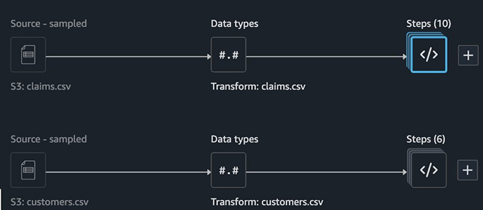
One of the outputs you can choose in SageMaker Data Wrangler is a Python notebook that distills these activities into a set of functions. The .flow file output contains a set of transformations that provide SageMaker Processing with guidance on what transformations to apply to features. The following screenshot shows the export options from SageMaker Data Wrangler.

We can send this code to SageMaker Processing to create a preprocessing job that prepares our datasets for training in a scalable and reproducible way.
Data prep
The following diagram shows the data prep architecture. The code is available in the notebook 1-data-prep-e2e.ipynb.

In the attached notebook for the data prep stage, we assume all the work was done in SageMaker Data Wrangler and the output is available in the /data folder of the example code, so you can follow the flow of the notebook. You can query, explore, and visualize features using SageMaker Data Wrangler from SageMaker Studio.
You can provide an S3 bucket that contains the results of the SageMaker Data Wrangler job that has output two files: claims.csv and customer.csv. If you want to move on and assume the data prep has been conducted, you can access the preprocessed data in the /data folder containing the files claims_preprocessed.csv (31 features) and customers_preprocessed.csv (19 features). The policy_id and event_time columns in customers_preprocessed.csv are necessary when creating a feature store, which requires a unique identifier for each record and a timestamp.
Dataset features and distribution
You can find the code for exploring the data in the notebook 0-AutoClaimFraudDetection.ipynb.
Here are some sample plots that indicate the nature of the class imbalance and to what features fraud may be correlated.
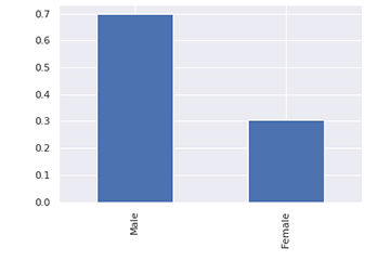
The dataset is heavily weighted towards male customers.
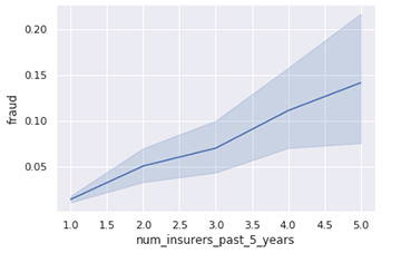
Fraud is positively correlated with having a greater number of insurers over the past 5 years. Customers who switched insurers more frequently also had more prevalence of fraud.
We loaded the raw data from the S3 bucket and created 10 transforms for claims and 6 for customers.
Transformations and featurizations
For claims, we formatted some strings and encoded several categorical features. See the following code:
Data columns (total 31 columns):
 #   Column                           Non-Null Count  Dtype
---  ------                           --------------  -----
 0   policy_id                        5000 non-null   int64
 1   incident_severity                5000 non-null   float64
 2   num_vehicles_involved            5000 non-null   int64
 3   num_injuries                     5000 non-null   int64
 4   num_witnesses                    5000 non-null   int64
 5   police_report_available          5000 non-null   float64
 6   injury_claim                     5000 non-null   int64
 7   vehicle_claim                    5000 non-null   int64
 8   total_claim_amount               5000 non-null   int64
 9   incident_month                   5000 non-null   int64
 10  incident_day                     5000 non-null   int64
 11  incident_dow                     5000 non-null   int64
 12  incident_hour                    5000 non-null   int64
 13  fraud                            5000 non-null   int64
 14  driver_relationship_self         5000 non-null   float64
 15  driver_relationship_na           5000 non-null   float64
 16  driver_relationship_spouse       5000 non-null   float64
 17  driver_relationship_child        5000 non-null   float64
 18  driver_relationship_other        5000 non-null   float64
 19  incident_type_collision          5000 non-null   float64
 20  incident_type_breakin            5000 non-null   float64
 21  incident_type_theft              5000 non-null   float64
 22  collision_type_front             5000 non-null   float64
 23  collision_type_rear              5000 non-null   float64
 24  collision_type_side              5000 non-null   float64
 25  collision_type_na                5000 non-null   float64
 26  authorities_contacted_police     5000 non-null   float64
 27  authorities_contacted_none       5000 non-null   float64
 28  authorities_contacted_fire       5000 non-null   float64
 29  authorities_contacted_ambulance  5000 non-null   float64
 30  event_time                       5000 non-null   float64
For customers, we have the following code:
#   Column                     Non-Null Count  Dtype
---  ------                     --------------  -----
 0   policy_id                  5000 non-null   int64
 1   customer_age               5000 non-null   int64
 2   customer_education         5000 non-null   int64
 3   months_as_customer         5000 non-null   int64
 4   policy_deductable          5000 non-null   int64
 5   policy_annual_premium      5000 non-null   int64
 6   policy_liability           5000 non-null   int64
 7   auto_year                  5000 non-null   int64
 8   num_claims_past_year       5000 non-null   int64
 9   num_insurers_past_5_years  5000 non-null   int64
 10  customer_gender_male       5000 non-null   float64
 11  customer_gender_female     5000 non-null   float64
 12  policy_state_ca            5000 non-null   float64
 13  policy_state_wa            5000 non-null   float64
 14  policy_state_az            5000 non-null   float64
 15  policy_state_or            5000 non-null   float64
 16  policy_state_nv            5000 non-null   float64
 17  policy_state_id            5000 non-null   float64
 18  event_time                 5000 non-null   float64
Preprocessing
Data is exported from SageMaker Data Wrangler into an S3 bucket. It’s then preprocessed using SageMaker Processing. We assume that the output of the preprocessing job has been deposited in the S3 bucket you provide, or you can find the preprocessed data in the /data folder.
Ingesting the preprocessed data into SageMaker Feature Store
After SageMaker Processing finishes the preprocessing and we have our two CSV data files for claims and customers ready. We have contributed to the standardization of these features by making them discoverable and reusable by ingesting them into SageMaker Feature Store.
SageMaker Feature Store is a centralized store for features and their associated metadata, allowing features to be easily discovered and reused across your organization or team. You have the option of creating an offline feature store (stored in Amazon S3) or an online component stored in a low-latency store, or both. Data is stored in your S3 bucket using a prefixing scheme based on event time. The offline feature store is append-only, which enables you to maintain a historical record of all feature values. Data is stored in the offline store in Parquet format for optimized storage and query access. SageMaker Feature Store supports combining data to produce, train, validate, and test datasets, and allows you to extract data at different points in time.
To store features, we first need to define their feature group. A feature group is the main feature store resource that contains the metadata for all the data stored in Amazon SageMaker Feature Store. A feature group is a logical grouping of features, defined in the feature store, to describe records. A feature group’s definition is composed of a list of feature definitions, a record identifier name, and configurations for its online and offline store.
The online database is optional, but very useful if you need supplemental features to be available at inference. In this section, we create two feature groups for our claims and customers datasets. After inserting the claims and customers data into their respective feature groups, you need to query the offline store with Amazon Athena to build the training dataset.
To ingest data, we first designate a feature group for each type of feature, in this case, one per CSV file. You can ingest data into feature groups in SageMaker Feature Store in one of two ways: streaming or batch. For this post, we use the batch method.
When the offline feature store is ready, a crawler catalogs it and loads the catalog into an Athena table. To construct the train and test datasets, we use a SQL query to join the claims and customers tables that were created in Athena.
Training and tuning
The code for this section can be found in the following notebooks: 2-lineage-train-assess-bias-tune-registry-e2e.ipynb and 3-mitigate-bias-train-model2-registry-e2e.ipynb. The following diagram illustrates the workflow for the bias check, training, tuning, lineage, and model registry stages.

We write the train and test split datasets to our designated S3 bucket, and create an XGBoost estimator to train our fraud detection model with a fraud or no fraud logistic target. Prior to starting the SageMaker training job using the built-in XGBoost algorithm, we set the XGBoost hyperparameters. You can learn more about XGBoost’s Learning Task Parameters, Tree Booster Parameters.
We take the opportunity to track all the artifacts or entities involved with the training job so we can track the lineage of the model. This is done by importing several sagemaker.lineage components. See the following code:
from sagemaker.lineage import context, artifact, association, action.Lineage Tracking provides us with visibility into the code, training data, and model artifacts that we then associate with association_type='Produced' and association_type='ContributesTo', which links what contributed to and what produced a given artifact in the process.
We also assess degrees of pre-training and post-training bias using SageMaker Clarify. Pre-training metrics show a variety of possible preexisting bias in our dataset. Post-training metrics show bias in the predictions resulting from the model. We use analysis_config.json to specify which groups we want to check bias across and which metrics we want to show.
We assess two metrics: the difference in positive proportions in predicted labels (DPPL) and if a class imbalance exists in the data. For our use case, we measure this on the gender feature, which indicates if we have more male customers than female customers. Results indicate a slight bias in our model measured by the DPPL metric.
Deploying and serving the model
The code for this section can be found in the notebook 4-deploy-run-inference-e2e.ipynb. The following diagram shows the deploy and serve stage for real-time inference.
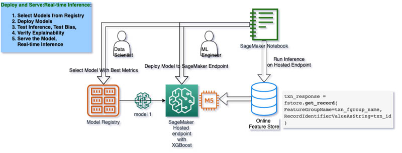
We choose the model that conforms to our metrics best, with an appropriate tolerance of F1 score, and deploy that model by creating a SageMaker training job that results in deploying the model to a SageMaker hosted endpoint.
When the endpoint is in place, we use the online feature store to run inference on the endpoint.
Interpreting the results
The following plot shows the data features and their relative impact on the prediction, using SHAP values.

We can trace back much of our interpretation of inference results to the features that had the most impact on the model output.
Creating an automated workflow using SageMaker Pipelines
The code for this section can be found in the notebook 5-pipeline-e2e.ipynb.
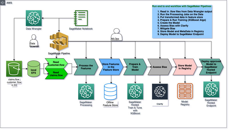
After we complete a few iterations of our manual exploratory data science and are happy with the outcomes of our cleansing, transformations, and featurizations, we may want to create an automated workflow using SageMaker Pipelines, so we can scale and don’t have to go through this manual process every time.
The following diagram shows our end-to-end automated MLOps pipeline, which includes eight steps:
- Preprocess the claims data with SageMaker Data Wrangler.
- Preprocess the customers data with SageMaker Data Wrangler.
- Create a dataset and train/test split.
- Train the XGBoost algorithm.
- Create the model.
- Run bias metrics with SageMaker Clarify.
- Register the model.
- Deploy the model.
Conclusion
In December 2020, AWS announced many new AI and ML services and features. In this post, we discussed how to build an end to end fraud detection use case for auto insurance claims using most of the these new capabilities including: SageMaker Data Wrangler for feature transformation, SageMaker Processing for preprocessing data, SageMaker Feature Store (offline) for standardization of features, SageMaker Clarify for bias detection pre- and post-training and for post-inference interpretability of results, ML Lineage Tracking to help with governance of ML artifacts, SageMaker Model Registry for model and metadata storage, and SageMaker Pipelines for end to end workflow automation. Additional information about each of these services can be found by checking out the following product page links.
- Amazon SageMaker Data Wrangler
- Amazon SageMaker Feature Store
- Amazon SageMaker Clarify
- Amazon SageMaker Pipelines
About the Author
 Dr. Ali Arsanjani is the Tech Sector AI/ML Leader and Principal Architect for AI/ML Specialist Solution Architects with AWS helping customers make optimal use of ML using the AWS platform. He is also an adjunct faculty member at San Jose State University, teaching and advising students in the Data Science Masters Programs.
