BERT, ELMo, & GPT-2: How Contextual are Contextualized Word Representations?

Incorporating context into word embeddings – as exemplified by BERT, ELMo, and GPT-2 – has proven to be a watershed idea in NLP. Replacing static vectors (e.g., word2vec) with contextualized word representations has led to significant improvements on virtually every NLP task.

But just how contextual are these contextualized representations?

Consider the word ‘mouse’. It has multiple word senses, one referring to a rodent and another to a device. Does BERT effectively create one representation of ‘mouse’ per word sense (left) ? Or does BERT create infinitely many representations of ‘mouse’, each highly specific to its context (right)?

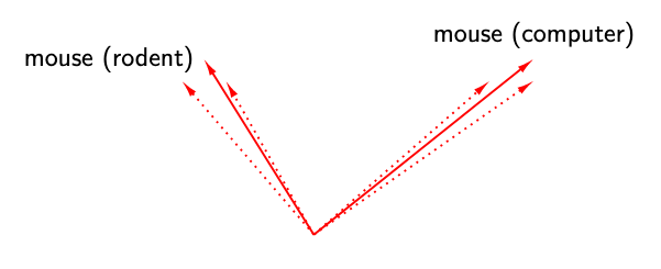
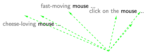
In our EMNLP 2019 paper, “How Contextual are Contextualized Word Representations?”, we tackle these questions and arrive at some surprising conclusions:

1. In all layers of BERT, ELMo, and GPT-2, the representations of all words are anisotropic: they occupy a narrow cone in the embedding space instead of being distributed throughout.

2. In all three models, upper layers produce more context-specific representations than lower layers; however, the models contextualize words very differently from one another.

3. If a word’s contextualized representations were not at all contextual, we’d expect 100% of their variance to be explained by a static embedding. Instead, we find that – on average – less than 5% of the variance can be explained by a static embedding.¹

4. We can create a new type of static embedding for each word by taking the first principal component of its contextualized representations in a lower layer of BERT. Static embeddings created this way outperform GloVe and FastText on benchmarks like solving word analogies!²

Going back to our example, this means that BERT creates highly context-specific representations of the word ‘mouse’ instead of creating one per word sense. Any static embedding of ‘mouse’ would account for very little of the variance in its contextualized representations. However, if we picked the vector that did maximize the variance explained, we would get a static embedding that is much better than the one provided by GloVe or FastText!³

Measures of Contextuality

What does contextuality look like? Consider these two sentences:

A panda dog runs.

A dog is trying to get bacon off its back.

== implies that there is no contextualization (i.e., what we’d get with word2vec).
!= implies that there is some contextualization. The difficulty lies in quantifying the extent to which this occurs. Since there is no definitive measure of contextuality, we propose three new ones:

1. Self-Similarity (SelfSim): The average cosine similarity of a word with itself across all the contexts in which it appears, where representations of the word are drawn from the same layer of a given model. For example, we would take the mean of cos(, ) over all unique pairs to calculate (‘dog’).

2. Intra-Sentence Similarity (IntraSim): The average cosine similarity between a word and its context. For the first sentence, where context vector :

   helps us discern whether the contextualization is naive – simply making each word more similar to its neighbors – or whether it is more nuanced, recognizing that words occurring in the same context can affect each other while still having distinct semantics.

3. Maximum Explainable Variance (MEV): The proportion of variance in a word’s representations that can be explained by their first principal component. For example, (‘dog’) would be the proportion of variance explained by the first principal component of , , and every other instance of ‘dog’ in the data. (‘dog’) = 1 would imply that there was no contextualization: a static embedding could replace all the contextualized representations. Conversely, if (‘dog’) were close to 0, then a static embedding could explain almost none of the variance.

Note that each of these measures is calculated for a given layer of a given model, since each layer has its own representation space. For example, the word ‘dog’ has different self-similarity values in Layer 1 of BERT and Layer 2 of BERT.

Adjusting for Anisotropy

When discussing contextuality, it is important to consider the isotropy of embeddings (i.e., whether they’re uniformly distributed in all directions).

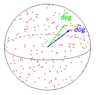
In both figures below, (‘dog’) = 0.95. The image on the left suggests that ‘dog’ is poorly contextualized. Not only are its representations nearly identical across all the contexts in which it appears, but the high isotropy of the representation space suggests that a self-similarity of 0.95 is exceptionally high. The image on the right suggests the opposite: because any two words have a cosine similarity over 0.95, ‘dog’ having a self-similarity of 0.95 is no longer impressive. Relative to other words, ‘dog’ would be considered highly contextualized!

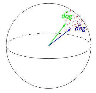
To adjust for anisotropy, we calculate anisotropic baselines for each of our measures and subtract each baseline from the respective raw measure.⁴

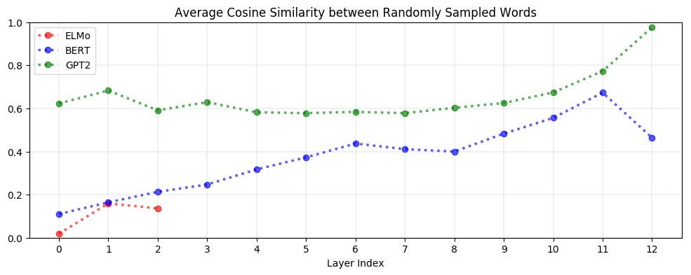
But is it even necessary to adjust for anisotropy? Yes! As seen below, upper layers of BERT and GPT-2 are extremely anisotropic, suggesting that high anisotropy is inherent to – or at least a consequence of – the process of contextualization:

Context-Specificity

On average, contextualized representations are more context-specific in higher layers. As seen below, the decrease in self-similarity is almost monotonic. This is analogous to how upper layers of LSTMs trained on NLP tasks learn more task-specific representations (Liu et al., 2019). GPT-2 is the most context-specific; representations in its last layer are almost maximally context-specific.

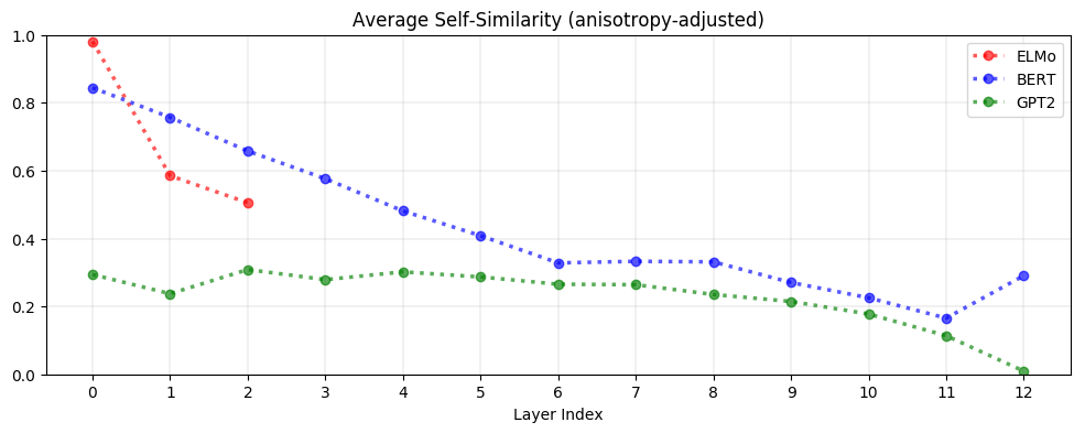
Stopwords such as ‘the’ have among the lowest self-similarity (i.e., the most context-specific representations). The variety of contexts a word appears in, rather than its inherent polysemy, is what drives variation in its contextualized representations. This suggests that ELMo, BERT, and GPT-2 are not simply assigning one representation per word sense; otherwise, there would not be so much variation in the representations of words with so few word senses.

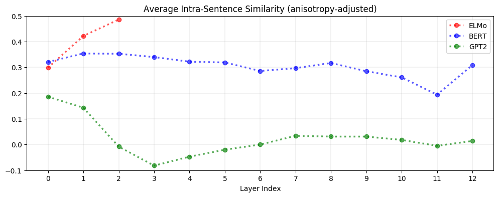
Context-specificity manifests very differently in ELMo, BERT, and GPT-2. As seen below, in ELMo, words in the same sentence are more similar to one another in upper layers. In BERT, words in the same sentence are more dissimilar to one another in upper layers but are on average more similar to each other than two random words. In contrast, for GPT-2, word representations in the same sentence are no more similar to each other than randomly sampled words. This suggests that BERT and GPT-2’s contextualization are more nuanced than ELMo’s, as they seem to recognize that words appearing in the same context do not necessarily have a similar meaning.

Static vs. Contextualized

On average, less than 5% of the variance in a word’s contextualized representations can be explained by a static embedding. If a word’s contextualized representations were not at all contextual, we would expect their first principal component to explain 100% of the variance. Instead, less than 5% of the variance can be explained on average. This 5% threshold represents the best-case scenario, where the static embedding is the first principal component. There is no theoretical guarantee that a GloVe vector, for example, is similar to the static embedding that maximizes the variance explained. This suggests that BERT, ELMo, and GPT-2 are not simply assigning one embedding per word sense: otherwise, the proportion of variance explained would be much higher.

Principal components of contextualized representations in lower layers of BERT outperform GloVe and FastText on many static embedding benchmarks. This method takes the previous finding to its logical conclusion: what if we created a new type of static embedding for each word by simply taking the first principal component of its contextualized representations? It turns out that this works surprisingly well. If we use representations from lower layers of BERT, these principal component embeddings outperform GloVe and FastText on benchmark tasks covering semantic similarity, analogy solving, and concept categorization (see table below).

For all three models, principal component embeddings created from lower layers are more effective than those created from upper layers. Those created using GPT-2 perform markedly worse than those from ELMo and BERT. Given that upper layers are much more context-specific than lower layers, and given that GPT-2’s representations are more context-specific, this suggests that principal components of less context-specific representations are more effective on these tasks.

Conclusion

In ELMo, BERT, and GPT-2, upper layers produce more context-specific representations than lower layers. However, these models contextualize words very differently from one another: after adjusting for anisotropy, the similarity between words in the same sentence is highest in ELMo but almost non-existent in GPT-2.

On average, less than 5% of the variance in a word’s contextualized representations can be explained by a static embedding. Even in the best-case scenario, static word embeddings would thus be a poor replacement for contextualized ones. Still, contextualized representations can be used to create a more powerful type of static embedding: principal components of contextualized representations in lower layers of BERT are much better than GloVe and FastText! If you’re interested in reading more along these lines, check out:

• The Dark Secrets of BERT (Rogers et al., 2019)
• Evolution of Representations in the Transformer (Voita et al., 2019)
• Cross-Lingual Alignment of Contextual Word Embeddings (Schuster et al., 2019)
• The Illustrated BERT, ELMo, and co. (Alammar, 2019)

Acknowledgements

Many thanks to Anna Rogers for live-tweeting this paper during EMNLP 2019. Special thanks to John Hewitt, Nelson Liu, and Krishnapriya Vishnubhotla for their comments on this blog post.

Read More