Time series are sequences of data points that occur in successive order over some period of time. We often analyze these data points to make better business decisions or gain competitive advantages. An example is Shimamura Music, who used Amazon Forecast to improve shortage rates and increase business efficiency. Another great example is Arneg, who used Forecast to predict maintenance needs.
AWS provides various services catered to time series data that are low code/no code, which both machine learning (ML) and non-ML practitioners can use for building ML solutions. These includes libraries and services like AutoGluon, Amazon SageMaker Canvas, Amazon SageMaker Data Wrangler, Amazon SageMaker Autopilot, and Amazon Forecast.
In this post, we seek to separate a time series dataset into individual clusters that exhibit a higher degree of similarity between its data points and reduce noise. The purpose is to improve accuracy by either training a global model that contains the cluster configuration or have local models specific to each cluster.
We explore how to extract characteristics, also called features, from time series data using the TSFresh library—a Python package for computing a large number of time series characteristics—and perform clustering using the K-Means algorithm implemented in the scikit-learn library.
We use the Time Series Clustering using TSFresh + KMeans notebook, which is available on our GitHub repo. We recommend running this notebook on Amazon SageMaker Studio, a web-based, integrated development environment (IDE) for ML.
Solution overview
Clustering is an unsupervised ML technique that groups items together based on a distance metric. The Euclidean distance is most commonly used for non-sequential datasets. However, because a time series inherently has a sequence (timestamp), the Euclidean distance doesn’t work well when used directly on time series because it’s invariant to time shifts, ignoring the time dimension of data. For a more detailed explanation, refer to Time Series Classification and Clustering with Python. A better distance metric that works directly on time series is Dynamic Time Warping (DTW). For an example of clustering based on this metric, refer to Cluster time series data for use with Amazon Forecast.
In this post, we generate features from the time series dataset using the TSFresh Python library for data extraction. TSFresh is a library that calculates a large number of time series characteristics, which include the standard deviation, quantile, and Fourier entropy, among others. This allows us to remove the time dimensionality of the dataset and apply common techniques that work for data with flattened formats. In addition to TSFresh, we also use StandardScaler, which standardizes features by removing the mean and scaling to unit variance, and Principal component analysis (PCA) to perform dimensionality reduction. Scaling reduces the distance between data points, which in turn promotes stability in the model training process, and dimensionality reduction allows the model to learn from fewer features while retaining the major trends and patterns, thereby enabling more efficient training.
Data loading
For this example, we use the UCI Online Retail II Data Set and perform basic data cleansing and preparation steps as detailed in the Data Cleaning and Preparation notebook.
Feature extraction with TSFresh
Let’s start by using TSFresh to extract features from our time series dataset:
Note that our data has been converted from a time series to a table comparing StockCode values vs. Feature values.

Next, we drop all features with n/a values by utilizing the dropna method:
Then we scale the features using StandardScaler. The values in the extracted features consist of both negative and positive values. Therefore, we use StandardScaler instead of MinMaxScaler:
We use PCA to do dimensionality reduction:
And we determine the optimal number of components for PCA:
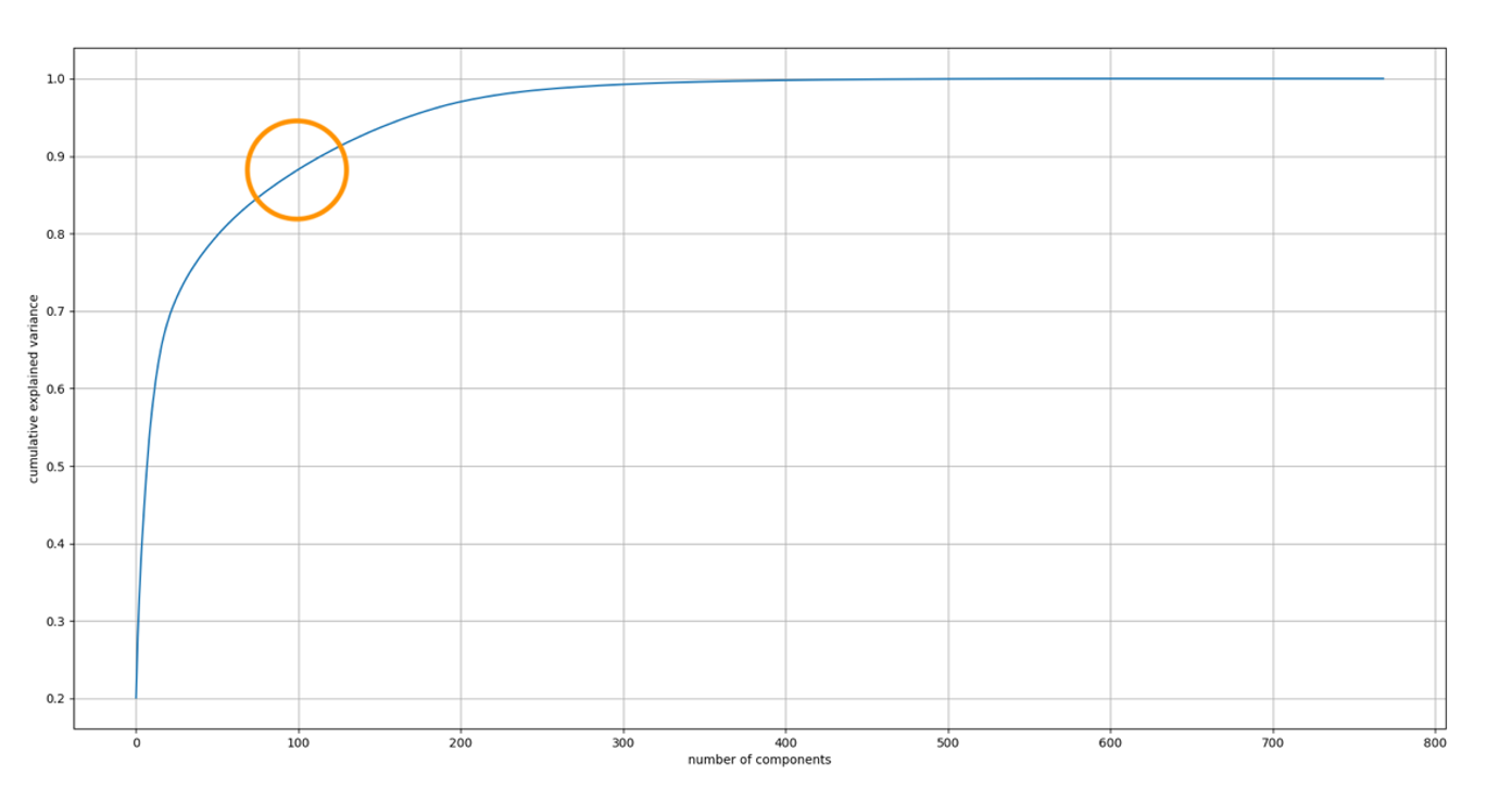
The explained variance ratio is the percentage of variance attributed to each of the selected components. Typically, you determine the number of components to include in your model by cumulatively adding the explained variance ratio of each component until you reach 0.8–0.9 to avoid overfitting. The optimal value usually occurs at the elbow.
As shown in the following chart, the elbow value is approximately 100. Therefore, we use 100 as the number of components for PCA.

Clustering with K-Means
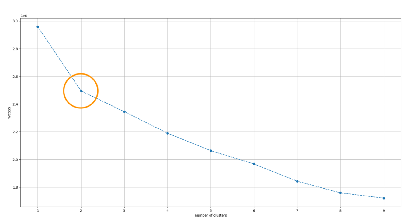
Now let’s use K-Means with the Euclidean distance metric for clustering. In the following code snippet, we determine the optimal number of clusters. Adding more clusters decreases the inertia value, but it also decreases the information contained in each cluster. Additionally, more clusters means more local models to maintain. Therefore, we want to have a small cluster size with a relatively low inertia value. The elbow heuristic works well for finding the optimal number of clusters.
The following chart visualizes our findings.

Based on this chart, we have decided to use two clusters for K-Means. We made this decision because the within-cluster sum of squares (WCSS) decreases at the highest rate between one and two clusters. It’s important to balance ease of maintenance with model performance and complexity, because although WCSS continues to decrease with more clusters, additional clusters increase the risk of overfitting. Furthermore, slight variations in the dataset can unexpectedly reduce accuracy.
It’s important to note that both clustering methods, K-Means with Euclidian distance (discussed in this post) and K-means algorithm with DTW, have their strengths and weaknesses. The best approach depends on the nature of your data and the forecasting methods you’re using. Therefore, we highly recommend experimenting with both approaches and comparing their performance to gain a more holistic understanding of your data.
Conclusion
In this post, we discussed the powerful techniques of feature extraction and clustering for time series data. Specifically, we showed how to use TSFresh, a popular Python library for feature extraction, to preprocess your time series data and obtain meaningful features.
When the clustering step is complete, you can train multiple Forecast models for each cluster, or use the cluster configuration as a feature. Refer to the Amazon Forecast Developer Guide for information about data ingestion, predictor training, and generating forecasts. If you have item metadata and related time series data, you can also include these as input datasets for training in Forecast. For more information, refer to Start your successful journey with time series forecasting with Amazon Forecast.
References
- Dua, D. and Graff, C. (2019). UCI Machine Learning Repository: http://archive.ics.uci.edu/ml. Irvine, CA: University of California, School of Information and Computer Science.
- Direct link to UCI dataset
- Scikit-learn GitHub repo
- TSFresh GitHub repo
About the Authors
 Aleksandr Patrushev is AI/ML Specialist Solutions Architect at AWS, based in Luxembourg. He is passionate about the cloud and machine learning, and the way they could change the world. Outside work, he enjoys hiking, sports, and spending time with his family.
 Chong En Lim is a Solutions Architect at AWS. He is always exploring ways to help customers innovate and improve their workflows. In his free time, he loves watching anime and listening to music.
 Egor Miasnikov is a Solutions Architect at AWS based in Germany. He is passionate about the digital transformation of our lives, businesses, and the world itself, as well as the role of artificial intelligence in this transformation. Outside of work, he enjoys reading adventure books, hiking, and spending time with his family.
