Fraudulent activities severely impact many industries, such as e-commerce, social media, and financial services. Frauds could cause a significant loss for businesses and consumers. American consumers reported losing more than $5.8 billion to frauds in 2021, up more than 70% over 2020. Many techniques have been used to detect fraudsters—rule-based filters, anomaly detection, and machine learning (ML) models, to name a few.
In real-world data, entities often involve rich relationships with other entities. Such a graph structure can provide valuable information for anomaly detection. For example, in the following figure, users are connected via shared entities such as Wi-Fi IDs, physical locations, and phone numbers. Due to the large number of unique values of these entities, like phone numbers, it’s difficult to use them in the traditional feature-based models—for example, one-hot encoding all phone numbers wouldn’t be viable. But such relationships could help predict whether a user is a fraudster. If a user has shared several entities with a known fraudster, the user is more likely a fraudster.
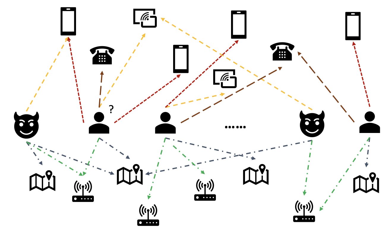
Recently, graph neural network (GNN) has become a popular method for fraud detection. GNN models can combine both graph structure and attributes of nodes or edges, such as users or transactions, to learn meaningful representations to distinguish malicious users and events from legitimate ones. This capability is crucial for detecting frauds where fraudsters collude to hide their abnormal features but leave some traces of relations.
Current GNN solutions mainly rely on offline batch training and inference mode, which detect fraudsters after malicious events have happened and losses have occurred. However, catching fraudulent users and activities in real time is crucial for preventing losses. This is particularly true in business cases where there is only one chance to prevent fraudulent activities. For example, in some e-commerce platforms, account registration is wide open. Fraudsters can behave maliciously just once with an account and never use the same account again.
Predicting fraudsters in real time is important. Building such a solution, however, is challenging. Because GNNs are still new to the industry, there are limited online resources on converting GNN models from batch serving to real-time serving. Additionally, it’s challenging to construct a streaming data pipeline that can feed incoming events to a GNN real-time serving API. To the best of the authors’ knowledge, no reference architectures and examples are available for GNN-based real-time inference solutions as of this writing.
To help developers apply GNNs to real-time fraud detection, this post shows how to use Amazon Neptune, Amazon SageMaker, and the Deep Graph Library (DGL), among other AWS services, to construct an end-to-end solution for real-time fraud detection using GNN models.
We focus on four tasks:
- Processing a tabular transaction dataset into a heterogeneous graph dataset
- Training a GNN model using SageMaker
- Deploying the trained GNN models as a SageMaker endpoint
- Demonstrating real-time inference for incoming transactions
This post extends the previous work in Detecting fraud in heterogeneous networks using Amazon SageMaker and Deep Graph Library, which focuses on the first two tasks. You can refer to that post for more details on heterogeneous graphs, GNNs, and semi-supervised training of GNNs.
Businesses looking for a fully-managed AWS AI service for fraud detection can also use Amazon Fraud Detector, which makes it easy to identify potentially fraudulent online activities, such as the creation of fake accounts or online payment fraud.
Solution overview
This solution contains two major parts.
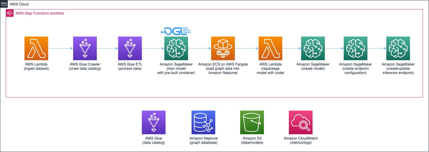
The first part is a pipeline that processes the data, trains GNN models, and deploys the trained models. It uses AWS Glue to process the transaction data, and saves the processed data to both Amazon Neptune and Amazon Simple Storage Service (Amazon S3). Then, a SageMaker training job is triggered to train a GNN model on the data saved in Amazon S3 to predict whether a transaction is fraudulent. The trained model along with other assets are saved back to Amazon S3 upon the completion of the training job. Finally, the saved model is deployed as a SageMaker endpoint. The pipeline is orchestrated by AWS Step Functions, as shown in the following figure.
The second part of the solution implements real-time fraudulent transaction detection. It starts from a RESTful API that queries the graph database in Neptune to extract the subgraph related to an incoming transaction. It also has a web portal that can simulate business activities, generating online transactions with both fraudulent and legitimate ones. The web portal provides a live visualization of the fraud detection. This part uses Amazon CloudFront, AWS Amplify, AWS AppSync, Amazon API Gateway, Step Functions, and Amazon DocumentDB to rapidly build the web application. The following diagram illustrates the real-time inference process and web portal.
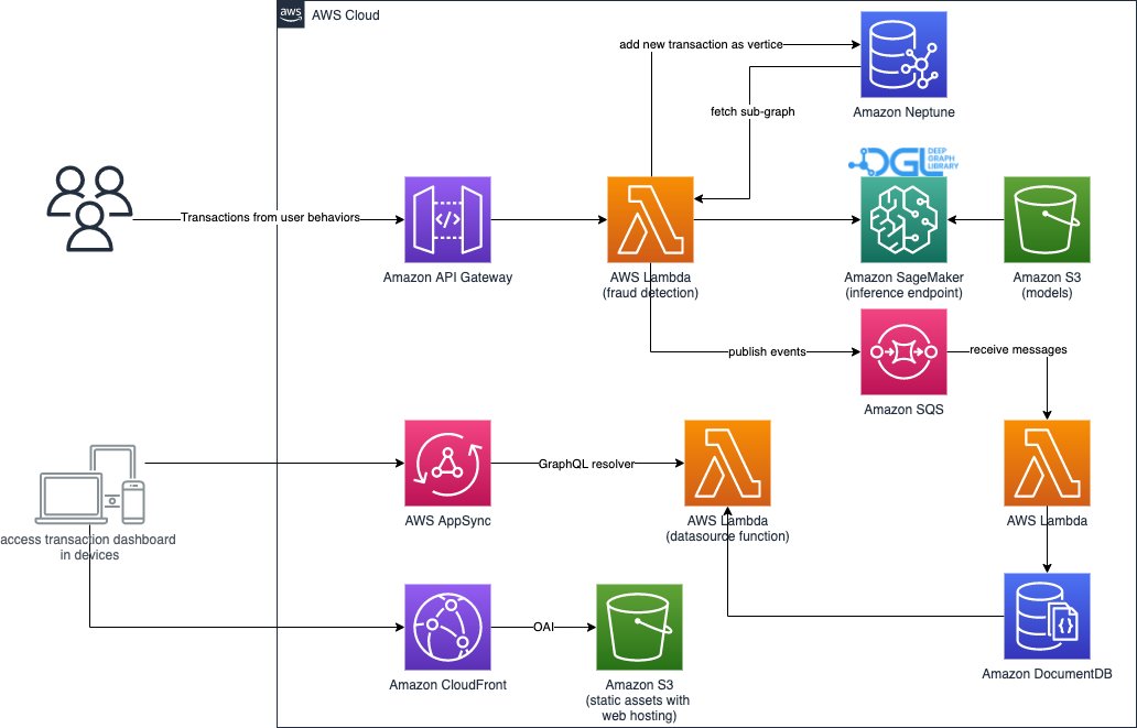
The implementation of this solution, along with an AWS CloudFormation template that can launch the architecture in your AWS account, is publicly available through the following GitHub repo.
Data processing
In this section, we briefly describe how to process an example dataset and convert it from raw tables into a graph with relations identified among different columns.
This solution uses the same dataset, the IEEE-CIS fraud dataset, as the previous post Detecting fraud in heterogeneous networks using Amazon SageMaker and Deep Graph Library. Therefore, the basic principle of the data process is the same. In brief, the fraud dataset includes a transactions table and an identities table, having nearly 500,000 anonymized transaction records along with contextual information (for example, devices used in transactions). Some transactions have a binary label, indicating whether a transaction is fraudulent. Our task is to predict which unlabeled transactions are fraudulent and which are legitimate.
The following figure illustrates the general process of how to convert the IEEE tables into a heterogeneous graph. We first extract two columns from each table. One column is always the transaction ID column, where we set each unique TransactionID as one node. Another column is picked from the categorical columns, such as the ProductCD and id_03 columns, where each unique category was set as a node. If a TransactionID and a unique category appear in the same row, we connect them with one edge. This way, we convert two columns in a table into one bipartite. Then we combine those bipartites along with the TransactionID nodes, where the same TransactionID nodes are merged into one unique node. After this step, we have a heterogeneous graph built from bipartites.
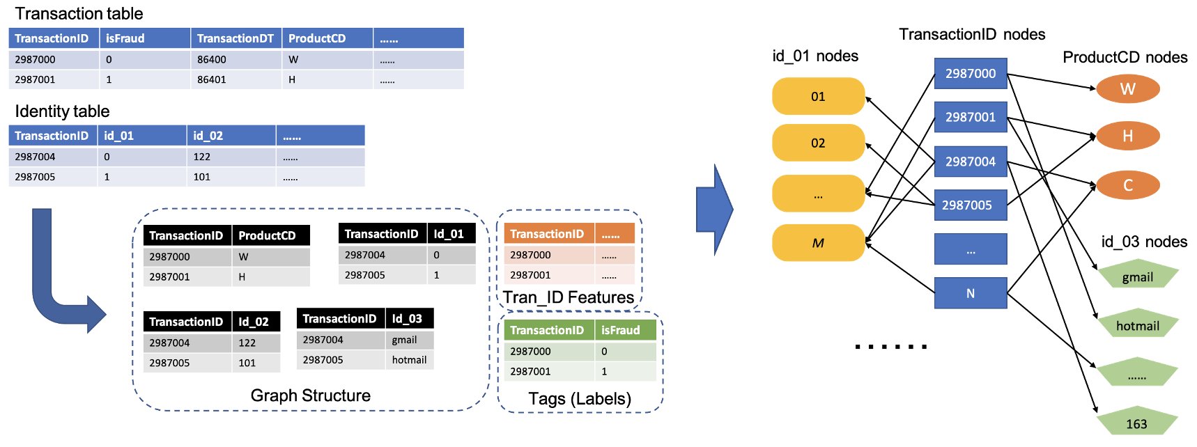
For the rest of the columns that aren’t used to build the graph, we join them together as the feature of the TransactionID nodes. TransactionID values that have the isFraud values are used as the label for model training. Based on this heterogeneous graph, our task becomes a node classification task of the TransactionID nodes. For more details on preparing the graph data for training GNNs, refer to the Feature extraction and Constructing the graph sections of the previous blog post.
The code used in this solution is available in src/scripts/glue-etl.py. You can also experiment with data processing through the Jupyter notebook src/sagemaker/01.FD_SL_Process_IEEE-CIS_Dataset.ipynb.
Instead of manually processing the data, as done in the previous post, this solution uses a fully automatic pipeline orchestrated by Step Functions and AWS Glue that supports processing huge datasets in parallel via Apache Spark. The Step Functions workflow is written in AWS Cloud Development Kit (AWS CDK). The following is a code snippet to create this workflow:
Besides constructing the graph data for GNN model training, this workflow also batch loads the graph data into Neptune to conduct real-time inference later on. This batch data loading process is demonstrated in the following code snippet:
GNN model training
After the graph data for model training is saved in Amazon S3, a SageMaker training job, which is only charged when the training job is running, is triggered to start the GNN model training process in the Bring Your Own Container (BYOC) mode. It allows you to pack your model training scripts and dependencies in a Docker image, which it uses to create SageMaker training instances. The BYOC method could save significant effort in setting up the training environment. In src/sagemaker/02.FD_SL_Build_Training_Container_Test_Local.ipynb, you can find details of the GNN model training.
Docker image
The first part of the Jupyter notebook file is the training Docker image generation (see the following code snippet):
We used a PyTorch-based image for the model training. The Deep Graph Library (DGL) and other dependencies are installed when building the Docker image. The GNN model code in the src/sagemaker/FD_SL_DGL/gnn_fraud_detection_dgl folder is copied to the image as well.
Because we process the transaction data into a heterogeneous graph, in this solution we choose the Relational Graph Convolutional Network (RGCN) model, which is specifically designed for heterogeneous graphs. Our RGCN model can train learnable embeddings for the nodes in heterogeneous graphs. Then, the learned embeddings are used as inputs of a fully connected layer for predicting the node labels.
Hyperparameters
To train the GNN, we need to define a few hyperparameters before the training process, such as the file names of the graph constructed, the number of layers of GNN models, the training epochs, the optimizer, the optimization parameters, and more. See the following code for a subset of the configurations:
For more information about all the hyperparameters and their default values, see estimator_fns.py in the src/sagemaker/FD_SL_DGL/gnn_fraud_detection_dgl folder.
Model training with SageMaker
After the customized container Docker image is built, we use the preprocessed data to train our GNN model with the hyperparameters we defined. The training job uses the DGL, with PyTorch as the backend deep learning framework, to construct and train the GNN. SageMaker makes it easy to train GNN models with the customized Docker image, which is an input argument of the SageMaker estimator. For more information about training GNNs with the DGL on SageMaker, see Train a Deep Graph Network.
The SageMaker Python SDK uses Estimator to encapsulate training on SageMaker, which runs SageMaker-compatible custom Docker containers, enabling you to run your own ML algorithms by using the SageMaker Python SDK. The following code snippet demonstrates training the model with SageMaker (either in a local environment or cloud instances):
After training, the GNN model’s performance on the test set is displayed like the following outputs. The RGCN model normally can achieve around 0.87 AUC and more than 95% accuracy. For a comparison of the RGCN model with other ML models, refer to the Results section of the previous blog post for more details.
Upon the completion of model training, SageMaker packs the trained model along with other assets, including the trained node embeddings, into a ZIP file and then uploads it to a specified S3 location. Next, we discuss the deployment of the trained model for real-time fraudulent detection.
GNN model deployment
SageMaker makes the deployment of trained ML models simple. In this stage, we use the SageMaker PyTorchModel class to deploy the trained model, because our DGL model depends on PyTorch as the backend framework. You can find the deployment code in the src/sagemaker/03.FD_SL_Endpoint_Deployment.ipynb file.
Besides the trained model file and assets, SageMaker requires an entry point file for the deployment of a customized model. The entry point file is run and stored in the memory of an inference endpoint instance to respond to the inference request. In our case, the entry point file is the fd_sl_deployment_entry_point.py file in the src/sagemaker/FD_SL_DGL/code folder, which performs four major functions:
- Receive requests and parse contents of requests to obtain the to-be-predicted nodes and their associated data
- Convert the data to a DGL heterogeneous graph as input for the RGCN model
- Perform the real-time inference via the trained RGCN model
- Return the prediction results to the requester
Following SageMaker conventions, the first two functions are implemented in the input_fn method. See the following code (for simplicity, we delete some commentary code):
The constructed DGL graph and features are then passed to the predict_fn method to fulfill the third function. predict_fn takes two input arguments: the outputs of input_fn and the trained model. See the following code:
The model used in perdict_fn is created by the model_fn method when the endpoint is called the first time. The function model_fn loads the saved model file and associated assets from the model_dir argument and the SageMaker model folder. See the following code:
The output of the predict_fn method is a list of two numbers, indicating the logits for class 0 and class 1, where 0 means legitimate and 1 means fraudulent. SageMaker takes this list and passes it to an inner method called output_fn to complete the final function.
To deploy our GNN model, we first wrap the GNN model into a SageMaker PyTorchModel class with the entry point file and other parameters (the path of the saved ZIP file, the PyTorch framework version, the Python version, and so on). Then we call its deploy method with instance settings. See the following code:
The preceding procedures and code snippets demonstrate how to deploy your GNN model as an online inference endpoint from a Jupyter notebook. However, for production, we recommend using the previously mentioned MLOps pipeline orchestrated by Step Functions for the entire workflow, including processing data, training the model, and deploying an inference endpoint. The entire pipeline is implemented by an AWS CDK application, which can be easily replicated in different Regions and accounts.
Real-time inference
When a new transaction arrives, to perform real-time prediction, we need to complete four steps:
- Node and edge insertion – Extract the transaction’s information such as the TransactionID and ProductCD as nodes and edges, and insert the new nodes into the existing graph data stored at the Neptune database.
- Subgraph extraction – Set the to-be-predicted transaction node as the center node, and extract a n-hop subgraph according to the GNN model’s input requirements.
- Feature extraction – For the nodes and edges in the subgraph, extract their associated features.
- Call the inference endpoint – Pack the subgraph and features into the contents of a request, then send the request to the inference endpoint.
In this solution, we implement a RESTful API to achieve real-time fraudulent predication described in the preceding steps. See the following pseudo-code for real-time predictions. The full implementation is in the complete source code file.
For prediction in real time, the first three steps require lower latency. Therefore, a graph database is an optimal choice for these tasks, particularly for the subgraph extraction, which could be achieved efficiently with graph database queries. The underline functions that support the pseudo-code are based on Neptune’s gremlin queries.
One caveat about real-time fraud detection using GNNs is the GNN inference mode. To fulfill real-time inference, we need to convert the GNN model inference from transductive mode to inductive mode. GNN models in transductive inference mode can’t make predictions for newly appeared nodes and edges, whereas in inductive mode, GNN models can handle new nodes and edges. A demonstration of the difference between transductive and inductive mode is shown in the following figure.
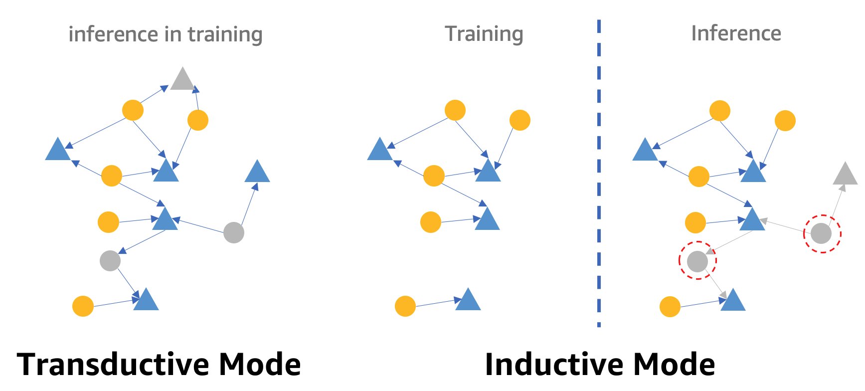
In transductive mode, predicted nodes and edges coexist with labeled nodes and edges during training. Models identify them before inference, and they could be inferred in training. Models in inductive mode are trained on the training graph but need to predict unseen nodes (those in red dotted circles on the right) with their associated neighbors, which might be new nodes, like the gray triangle node on the right.
Our RGCN model is trained and tested in transductive mode. It has access to all nodes in training, and also trained an embedding for each featureless node, such as IP address and card types. In the testing stage, the RGCN model uses these embeddings as node features to predict nodes in the test set. When we do real-time inference, however, some of the newly added featureless nodes have no such embeddings because they’re not in the training graph. One way to tackle this issue is to assign the mean of all embeddings in the same node type to the new nodes. In this solution, we adopt this method.
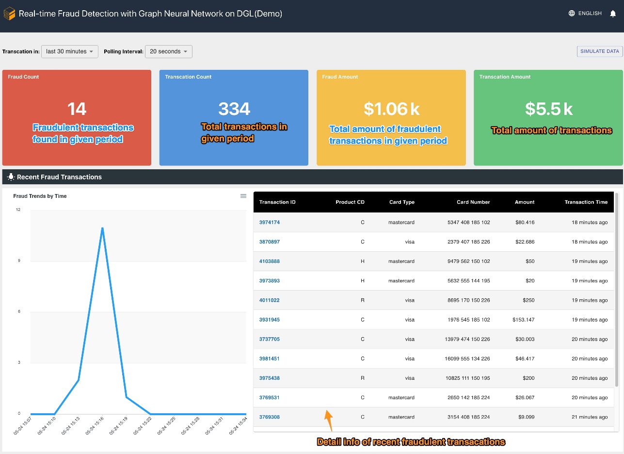
In addition, this solution provides a web portal (as seen in the following screenshot) to demonstrate real-time fraudulent predictions from business operators’ perspectives. It can generate the simulated online transactions, and provide a live visualization of detected fraudulent transaction information.
Clean up
When you’re finished exploring the solution, you can clean the resources to avoid incurring charges.
Conclusion
In this post, we showed how to build a GNN-based real-time fraud detection solution using SageMaker, Neptune, and the DGL. This solution has three major advantages:
- It has good performance in terms of prediction accuracy and AUC metrics
- It can perform real-time inference via a streaming MLOps pipeline and SageMaker endpoints
- It automates the total deployment process with the provided CloudFormation template so that interested developers can easily test this solution with custom data in their account
For more details about the solution, see the GitHub repo.
After you deploy this solution, we recommend customizing the data processing code to fit your own data format and modify the real-time inference mechanism while keeping the GNN model unchanged. Note that we split the real-time inference into four steps without further optimization of the latency. These four steps take a few seconds to get a prediction on the demo dataset. We believe that optimizing the Neptune graph data schema design and queries for subgraph and feature extraction can significantly reduce the inference latency.
About the authors
 Jian Zhang is an applied scientist who has been using machine learning techniques to help customers solve various problems, such as fraud detection, decoration image generation, and more. He has successfully developed graph-based machine learning, particularly graph neural network, solutions for customers in China, USA, and Singapore. As an enlightener of AWS’s graph capabilities, Zhang has given many public presentations about the GNN, the Deep Graph Library (DGL), Amazon Neptune, and other AWS services.
 Mengxin Zhu is a manager of Solutions Architects at AWS, with a focus on designing and developing reusable AWS solutions. He has been engaged in software development for many years and has been responsible for several startup teams of various sizes. He also is an advocate of open-source software and was an Eclipse Committer.
 Haozhu Wang is a research scientist at Amazon ML Solutions Lab, where he co-leads the Reinforcement Learning Vertical. He helps customers build advanced machine learning solutions with the latest research on graph learning, natural language processing, reinforcement learning, and AutoML. Haozhu received his PhD in Electrical and Computer Engineering from the University of Michigan.
