Build a risk management machine learning workflow on Amazon SageMaker with no code

Since the global financial crisis, risk management has taken a major role in shaping decision-making for banks, including predicting loan status for potential customers. This is often a data-intensive exercise that requires machine learning (ML). However, not all organizations have the data science resources and expertise to build a risk management ML workflow.

Amazon SageMaker is a fully managed ML platform that allows data engineers and business analysts to quickly and easily build, train, and deploy ML models. Data engineers and business analysts can collaborate using the no-code/low-code capabilities of SageMaker. Data engineers can use Amazon SageMaker Data Wrangler to quickly aggregate and prepare data for model building without writing code. Then business analysts can use the visual point-and-click interface of Amazon SageMaker Canvas to generate accurate ML predictions on their own.

In this post, we show how simple it is for data engineers and business analysts to collaborate to build an ML workflow involving data preparation, model building, and inference without writing code.

Solution overview

Although ML development is a complex and iterative process, you can generalize an ML workflow into the data preparation, model development, and model deployment stages.

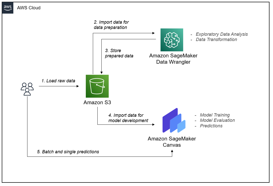
Data Wrangler and Canvas abstract the complexities of data preparation and model development, so you can focus on delivering value to your business by drawing insights from your data without being an expert in code development. The following architecture diagram highlights the components in a no-code/low-code solution.

Amazon Simple Storage Service (Amazon S3) acts as our data repository for raw data, engineered data, and model artifacts. You can also choose to import data from Amazon Redshift, Amazon Athena, Databricks, and Snowflake.

As data scientists, we then use Data Wrangler for exploratory data analysis and feature engineering. Although Canvas can run feature engineering tasks, feature engineering usually requires some statistical and domain knowledge to enrich a dataset into the right form for model development. Therefore, we give this responsibility to data engineers so they can transform data without writing code with Data Wrangler.

After data preparation, we pass model building responsibilities to data analysts, who can use Canvas to train a model without having to write any code.

Finally, we make single and batch predictions directly within Canvas from the resulting model without having to deploy model endpoints ourselves.

Dataset overview

We use SageMaker features to predict the status of a loan using a modified version of Lending Club’s publicly available loan analysis dataset. The dataset contains loan data for loans issued through 2007–2011. The columns describing the loan and the borrower are our features. The column loan_status is the target variable, which is what we’re trying to predict.

To demonstrate in Data Wrangler, we split the dataset in two CSV files: part one and part two. We’ve removed some columns from Lending Club’s original dataset to simplify the demo. Our dataset contains over 37,000 rows and 21 feature columns, as described in the following table.

We use this dataset for our data preparation and model training.

Prerequisites

Complete the following prerequisite steps:

1. Upload both loan files to an S3 bucket of your choice.
2. Make sure you have the necessary permissions. For more information, refer to Get Started with Data Wrangler.
3. Set up a SageMaker domain configured to use Data Wrangler. For instructions, refer to Onboard to Amazon SageMaker Domain.

Import the data

Create a new Data Wrangler data flow from the Amazon SageMaker Studio UI.

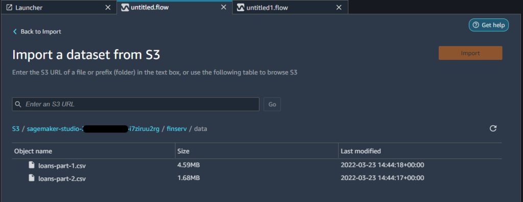
Import data from Amazon S3 by selecting the CSV files from the S3 bucket where you placed your dataset. After you import both files, you can see two separate workflows in the Data flow view.

You can choose several sampling options when importing your data in a Data Wrangler flow. Sampling can help when you have a dataset that is too large to prepare interactively, or when you want to preserve the proportion of rare events in your sampled dataset. Because our dataset is small, we don’t use sampling.

Prepare the data

For our use case, we have two datasets with a common column: id. As a first step in data preparation, we want to combine these files by joining them. For instructions, refer to Transform Data.

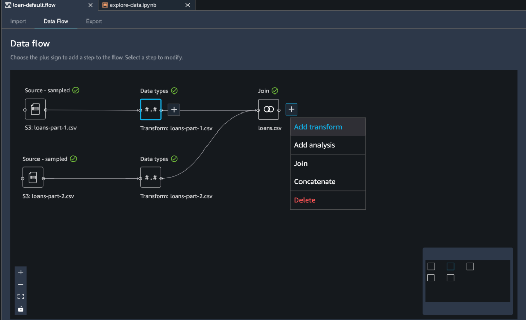
We use the Join data transformation step and use the Inner join type on the id column.

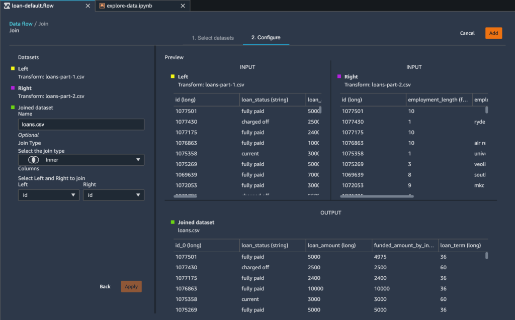
As a result of our join transformation, Data Wrangler creates two additional columns: id_0 and id_1. However, these columns are unnecessary for our model building purposes. We drop these redundant columns using the Manage columns transform step.

We’ve imported our datasets, joined them, and removed unnecessary columns. We’re now ready to enrich our data through feature engineering and prepare for model building.

Perform feature engineering

We used Data Wrangler for preparing data. You can also use the Data Quality and Insights Report feature within Data Wrangler to verify your data quality and detect abnormalities in your data. Data scientists often need to use these data insights to efficiently apply the right domain knowledge to engineering features. For this post, we assume we’ve completed these quality assessments and can move on to feature engineering.

In this step, we apply a few transformations to numeric, categorical, and text columns.

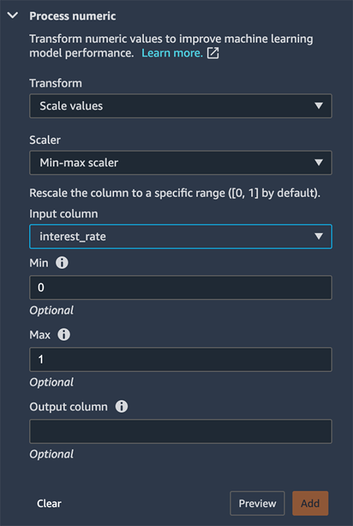
We first normalize the interest rate to scale the values between 0–1. We do this using the Process numeric transform to scale the interest_rate column using a min-max scaler. The purpose for normalization (or standardization) is to eliminate bias from our model. Variables that are measured at different scales won’t contribute equally to the model learning process. Therefore, a transformation function like a min-max scaler transform helps normalize features.

To convert a categorial variable into a numeric value, we use one-hot encoding. We choose the Encode categorical transform, then choose One-hot encode. One-hot encoding improves an ML model’s predictive ability. This process converts a categorical value into a new feature by assigning a binary value of 1 or 0 to the feature. As a simple example, if you had one column that held either a value of yes or no, one-hot encoding would convert that column to two columns: a Yes column and a No column. A yes value would have 1 in the Yes column and a 0 in the No column. One-hot encoding makes our data more useful because numeric values can more easily determine a probability for our predictions.

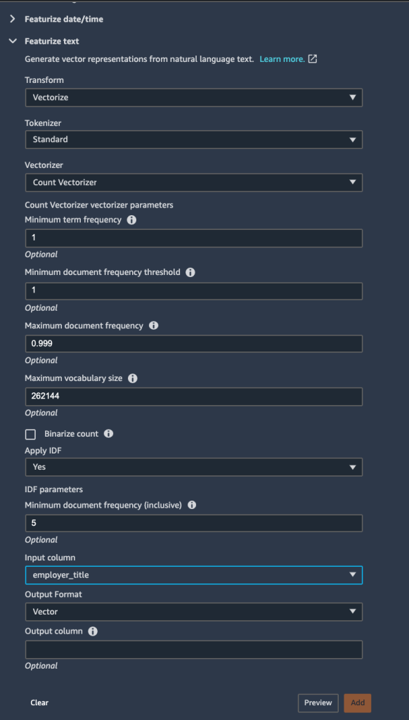
Finally, we featurize the employer_title column to transform its string values into a numerical vector. We apply the Count Vectorizer and a standard tokenizer within the Vectorize transform. Tokenization breaks down a sentence or series of text into words, whereas a vectorizer converts text data into a machine-readable form. These words are represented as vectors.

With all feature engineering steps complete, we can export the data and output the results into our S3 bucket. Alternatively, you can export your flow as Python code, or a Jupyter notebook to create a pipeline with your view using Amazon SageMaker Pipelines. Consider this when you want to run your feature engineering steps at scale or as part of an ML pipeline.

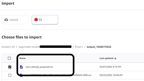
We can now use the Data Wrangler output file as our input for Canvas. We reference this as a dataset in Canvas to build our ML model.

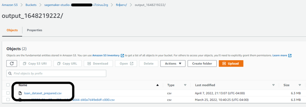
In our case, we exported our prepared dataset to the default Studio bucket with an output prefix. We reference this dataset location when loading the data into Canvas for model building next.

Build and train your ML model with Canvas

On the SageMaker console, launch the Canvas application. To build an ML model from the prepared data in the previous section, we perform the following steps:

1. Import the prepared dataset to Canvas from the S3 bucket.

We reference the same S3 path where we exported the Data Wrangler results from the previous section.

2. Create new model in Canvas and name it loan_prediction_model.
3. Select the imported dataset and add it to the model object.

To have Canvas build a model, we must select the target column.

4. Because our goal is to predict the probability of a lender’s ability to repay a loan, we choose the loan_status column.

Canvas automatically identifies the type of ML problem statement. At the time of writing, Canvas supports regression, classification, and time series forecasting problems. You can specify the type of problem or have Canvas automatically infer the problem from your data.

5. Choose your option to start the model building process: Quick build or Standard build.

The Quick build option uses your dataset to train a model within 2–15 minutes. This is useful when you’re experimenting with a new dataset to determine if the dataset you have will be sufficient to make predictions. We use this option for this post.

The Standard build option choses accuracy over speed and uses approximately 250 model candidates to train the model. The process usually takes 1–2 hours.

After the model is built, you can review the results of the model. Canvas estimates that your model is able to predict the right outcome 82.9% of the time. Your own results may vary due to the variability in training models.

In addition, you can dive deep into details analysis of the model to learn more about the model.

Feature importance represents the estimated importance of each feature in predicting the target column. In this case, the credit line column has the most significant impact in predicting if a customer will pay back the loan amount, followed by interest rate and annual income.

The confusion matrix in the Advanced metrics section contains information for users that want a deeper understanding of their model performance.

Before you can deploy your model for production workloads, use Canvas to test the model. Canvas manages our model endpoint and allows us to make predictions directly in the Canvas user interface.

6. Choose Predict and review the findings on either the Batch prediction or Single prediction tab.

In the following example, we make a single prediction by modifying values to predict our target variable loan_status in real time

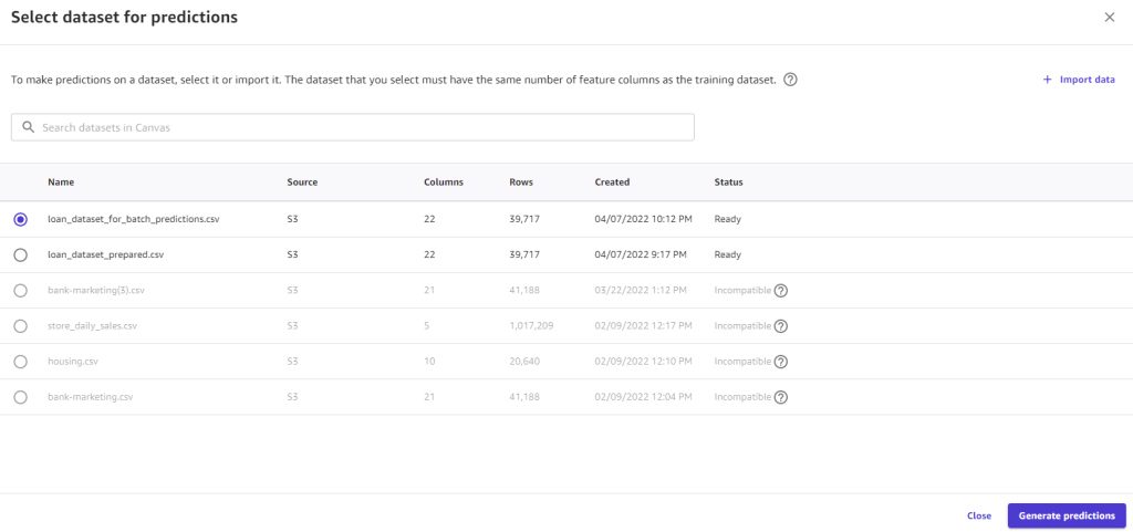
We can also select a larger dataset and have Canvas generate batch predictions on our behalf.

Conclusion

End-to-end machine learning is complex and iterative, and often involves multiple personas, technologies, and processes. Data Wrangler and Canvas enable collaboration between teams without requiring these teams to write any code.

A data engineer can easily prepare data using Data Wrangler without writing any code and pass the prepared dataset to a business analyst. A business analyst can then easily build accurate ML models with just a few click using Canvas and get accurate predictions in real time or in batch.

Get started with Data Wrangler using these tools without having to manage any infrastructure. You can set up Canvas quickly and immediately start creating ML models to support your business needs.

About the Authors

Peter Chung is a Solutions Architect for AWS, and is passionate about helping customers uncover insights from their data. He has been building solutions to help organizations make data-driven decisions in both the public and private sectors. He holds all AWS certifications as well as two GCP certifications.

 Meenakshisundaram Thandavarayan is a Senior AI/ML specialist with AWS. He helps hi-tech strategic accounts on their AI and ML journey. He is very passionate about data-driven AI.

Dan Ferguson is a Solutions Architect at AWS, based in New York, USA. As a machine learning services expert, Dan works to support customers on their journey to integrating ML workflows efficiently, effectively, and sustainably.

Read More