Image classification is a computer vision-based machine learning (ML) technique that allows you to classify images. Some well-known examples of image classification include classifying handwritten digits, medical image classification, and facial recognition. Image classification is a useful technique with several business applications, but building a good image classification model isn’t trivial.
Several considerations can play a role when evaluating an ML model. Beyond model accuracy, other potential metrics of importance are model training time and inference time. Given the iterative nature of ML model development, faster training times allow data scientists to quickly test various hypotheses. Faster inferencing can be critical in real-time applications.
Amazon SageMaker JumpStart provides one-click fine-tuning and deployment of a wide variety of pre-trained models across popular ML tasks, as well as a selection of end-to-end solutions that solve common business problems. These features remove the heavy lifting from each step of the ML process, making it easier to develop high-quality models and reducing time to deployment. JumpStart APIs allow you to programmatically deploy and fine-tune a vast selection of JumpStart-supported pre-trained models on your own datasets.
You can incrementally train and tune the ML models offered in JumpStart before deployment. At the time of writing, 87 deep-learning based image classification models are available in JumpStart.
But which model will give you the best results? In this post, we present a methodology to easily run multiple models and compare their outputs on three dimensions of interest: model accuracy, training time, and inference time.
Solution overview
JumpStart allows you to train, tune, and deploy models either from the JumpStart console using its UI or with its API. In this post, we use the API route, and present a notebook with various helper scripts. You can run this notebook and get results for easy comparison of these models against each other, and then pick a model that best suits your business need in terms of model accuracy, training time, and inference time.
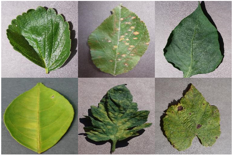
The public dataset used in this post consists of nearly 55,000 images of diseased and healthy plant leaves collected under controlled conditions, with class labels ranging from 0–38. This dataset is divided into train and validation datasets, with approximately 44,000 under training and 11,000 images under validation. The following are a few sample images.
For this exercise, we selected models from two frameworks—PyTorch and TensorFlow—as offered by JumpStart. The following 15 model algorithms cover a wide range of popular neural network architectures from these frameworks:
pytorch-ic-alexnet-FTpytorch-ic-densenet121-FTpytorch-ic-densenet201-FTpytorch-ic-googlenet-FTpytorch-ic-mobilenet-v2-FTpytorch-ic-resnet152-FTpytorch-ic-resnet34-FTtensorflow-ic-bit-s-r101x1-ilsvrc2012-classification-1-FTtensorflow-ic-imagenet-inception-resnet-v2-classification 4-FTtensorflow-ic-imagenet-inception-v3-classification-4-FTtensorflow-ic-imagenet-mobilenet-v2-050-224-classification-4-FTtensorflow-ic-imagenet-mobilenet-v2-075-224-classification-4-FTtensorflow-ic-imagenet-mobilenet-v2-140-224-classification-4-FTtensorflow-ic-imagenet-resnet-v2-152-classification-4-FTtensorflow-ic-tf2-preview-mobilenet-v2-classification-4-FT
We use the model tensorflow-ic-imagenet-inception-v3-classification-4-FT as a base against which results from other models are compared. This base model was picked arbitrarily.
The code used to run this comparison is available on the AWS Samples GitHub repo.
Results
In this section, we present the results from these 15 runs. For all these runs, the hyperparameters used were epochs = 5, learning rate = 0.001, batch size = 16.
Model accuracy, training time, and inference time from model tensorflow-ic-imagenet-inception-v3-classification-4-FT were taken as the base, and results from all other models are presented relative to this base model. Our intention here is not to show which model is the best but to rather show how, through the JumpStart API, you can compare results from various models and then choose a model that best fits your use case.
The following screenshot highlights the base model against which all other models were compared.
The following plot shows a detailed view of relative accuracy vs. relative training time. PyTorch models are color coded in red and TensorFlow models in blue.
The models highlighted with a green ellipse in the preceding plot seem to have a good combination of relative accuracy and low relative training time. The following table provides more details on these three models.
| Model Name | Relative Accuracy | Relative Training Time |
| tensorflow-ic-imagenet-mobilenet-v2-050-224-classification-4-FT | 1.01 | 0.74 |
| tensorflow-ic-imagenet-mobilenet-v2-140-224-classification-4-FT | 1.02 | 0.74 |
| tensorflow-ic-bit-s-r101x1-ilsvrc2012-classification-1-FT | 1.04 | 1.16 |
The following plot compares relative accuracy vs. relative inference time. PyTorch models are color coded in red and TensorFlow models in blue.
The following table provides details on the three models in the green ellipse.
| Model Name | Relative Accuracy | Relative Inference Time |
| tensorflow-ic-imagenet-mobilenet-v2-050-224-classification-4-FT | 1.01 | 0.94 |
| tensorflow-ic-imagenet-mobilenet-v2-140-224-classification-4-FT | 1.02 | 0.90 |
| tensorflow-ic-bit-s-r101x1-ilsvrc2012-classification-1-FT | 1.04 | 1.43 |
The two plots clearly demonstrate that certain model algorithms performed better than others on the three dimensions that were selected. The flexibility offered through this exercise can help you pick the right algorithm, and by using the provided notebook, you can easily run this type of experiment on any of the 87 available models.
Conclusion
In this post, we showed how to use JumpStart to build high performing image classification models on multiple dimensions of interest, such as model accuracy, training time, and inference latency. We also provided the code to run this exercise on your own dataset; you can pick any models of interest from the 87 models that are presently available for image classification in the JumpStart model hub. We encourage you to give it a try today.
For more details on JumpStart, refer to SageMaker JumpStart.
About the Authors
 Dr. Raju Penmatcha is an AI/ML Specialist Solutions Architect in AI Platforms at AWS. He received his PhD from Stanford University. He works closely on the low/no-code suite of services in SageMaker, which help customers easily build and deploy machine learning models and solutions. When not helping customers, he likes traveling to new places.
 Dr. Ashish Khetan is a Senior Applied Scientist with Amazon SageMaker built-in algorithms and helps develop machine learning algorithms. He got his PhD from University of Illinois Urbana-Champaign. He is an active researcher in machine learning and statistical inference, and has published many papers in NeurIPS, ICML, ICLR, JMLR, ACL, and EMNLP conferences.


