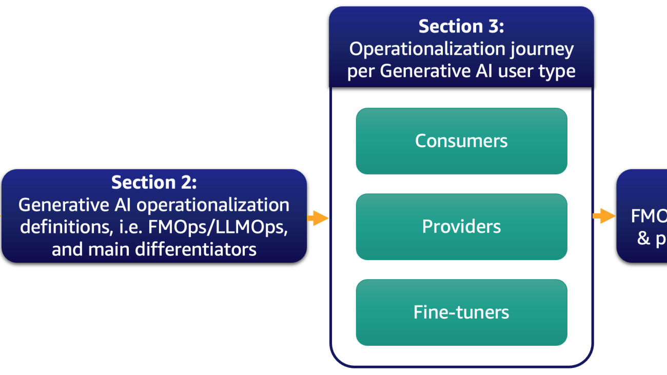
Nowadays, the majority of our customers is excited about large language models (LLMs) and thinking how generative AI could transform their business. However, bringing such solutions and models to the business-as-usual operations is not an easy task. In this post, we discuss how to operationalize generative AI applications using MLOps principles leading to foundation model operations (FMOps). Furthermore, we deep dive on the most common generative AI use case of text-to-text applications and LLM operations (LLMOps), a subset of FMOps. The following figure illustrates the topics we discuss.
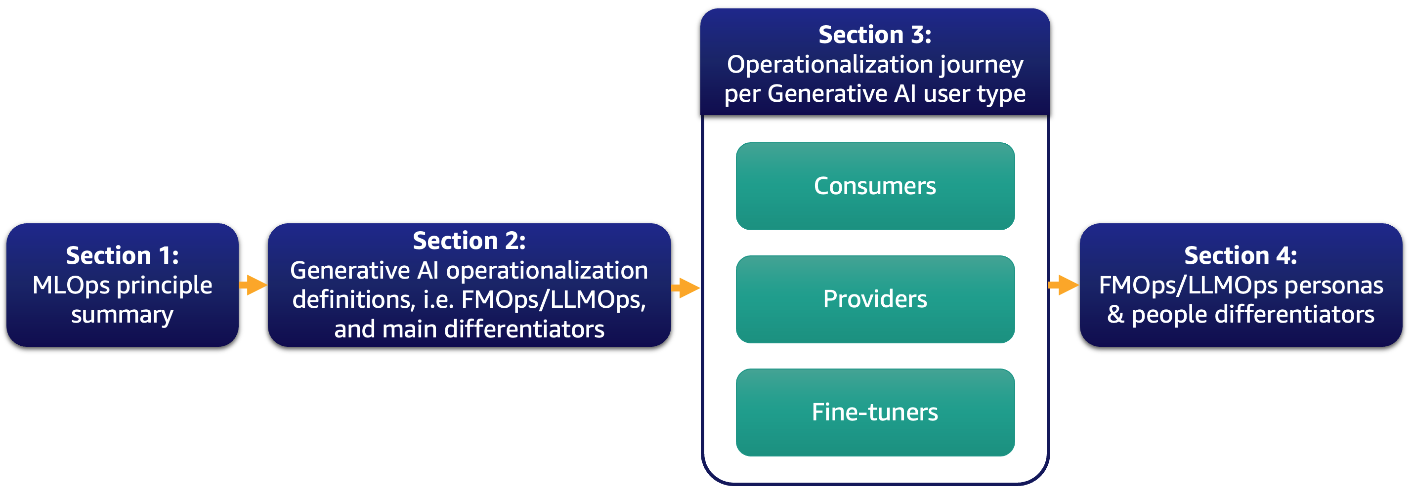
Specifically, we briefly introduce MLOps principles and focus on the main differentiators compared to FMOps and LLMOps regarding processes, people, model selection and evaluation, data privacy, and model deployment. This applies to customers that use them out of the box, create foundation models from scratch, or fine-tune them. Our approach applies to both open-source and proprietary models equally.
ML operationalization summary
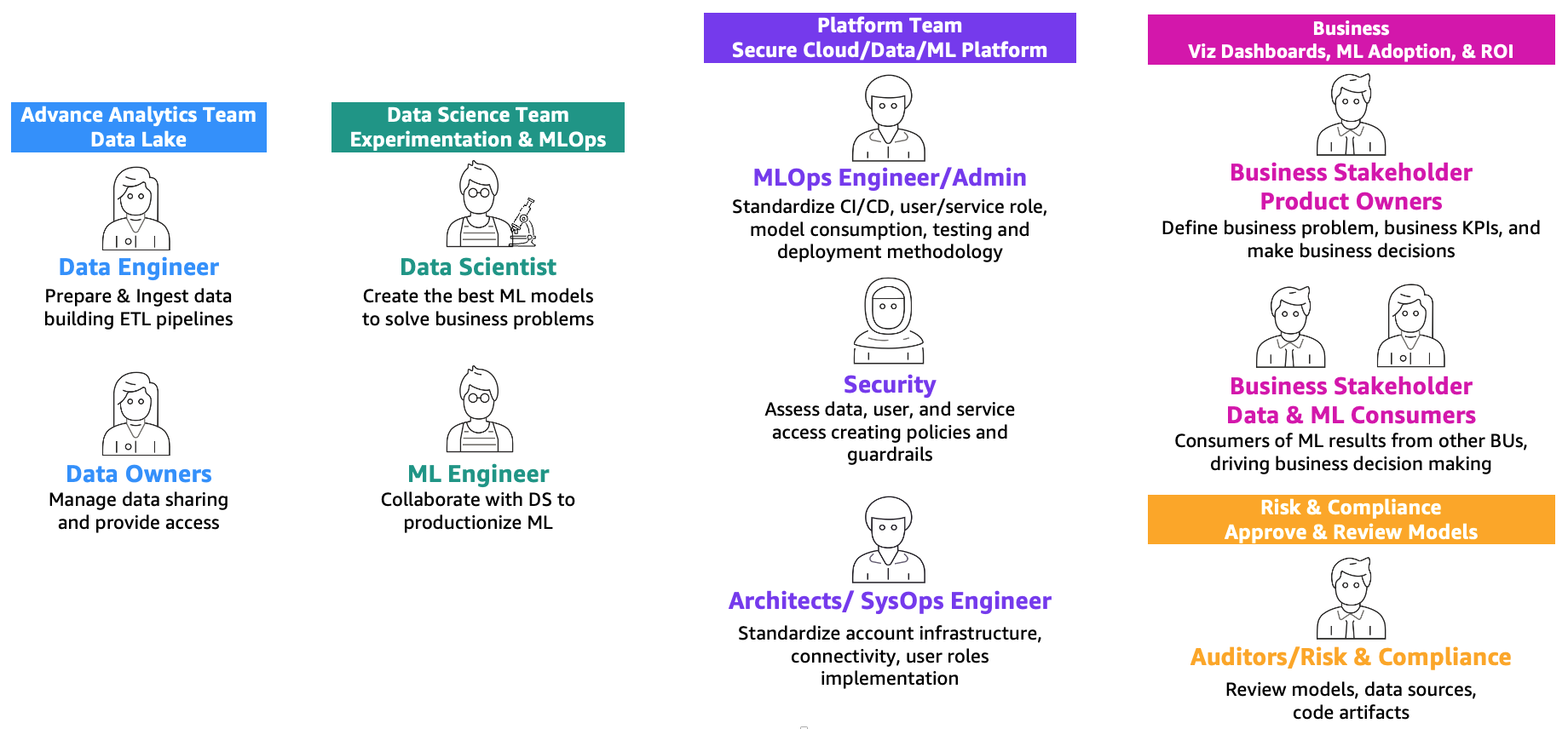
As defined in the post MLOps foundation roadmap for enterprises with Amazon SageMaker, ML and operations (MLOps) is the combination of people, processes, and technology to productionize machine learning (ML) solutions efficiently. To achieve this, a combination of teams and personas need to collaborate, as illustrated in the following figure.
These teams are as follows:
- Advanced analytics team (data lake and data mesh) – Data engineers are responsible for preparing and ingesting data from multiple sources, building ETL (extract, transform, and load) pipelines to curate and catalog the data, and prepare the necessary historical data for the ML use cases. These data owners are focused on providing access to their data to multiple business units or teams.
- Data science team – Data scientists need to focus on creating the best model based on predefined key performance indicators (KPIs) working in notebooks. After the completion of the research phase, the data scientists need to collaborate with ML engineers to create automations for building (ML pipelines) and deploying models into production using CI/CD pipelines.
- Business team – A product owner is responsible for defining the business case, requirements, and KPIs to be used to evaluate model performance. The ML consumers are other business stakeholders who use the inference results (predictions) to drive decisions.
- Platform team – Architects are responsible for the overall cloud architecture of the business and how all the different services are connected together. Security SMEs review the architecture based on business security policies and needs. MLOps engineers are responsible for providing a secure environment for data scientists and ML engineers to productionize the ML use cases. Specifically, they are responsible for standardizing CI/CD pipelines, user and service roles and container creation, model consumption, testing, and deployment methodology based on business and security requirements.
- Risk and compliance team – For more restrictive environments, auditors are responsible for assessing the data, code, and model artifacts and making sure that the business is compliant with regulations, such as data privacy.
Note that multiple personas can be covered by the same person depending on the scaling and MLOps maturity of the business.
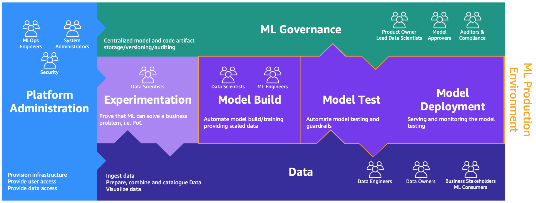
These personas need dedicated environments to perform the different processes, as illustrated in the following figure.
The environments are as follows:
- Platform administration – The platform administration environment is the place where the platform team has access to create AWS accounts and link the right users and data
- Data – The data layer, often known as the data lake or data mesh, is the environment that data engineers or owners and business stakeholders use to prepare, interact, and visualize with the data
- Experimentation – The data scientists use a sandbox or experimentation environment to test new libraries and ML techniques to prove that their proof of concept can solve business problems
- Model build, model test, model deployment – The model build, test, and deployment environment is the layer of MLOps, where data scientists and ML engineers collaborate to automate and move the research to production
- ML governance – The last piece of the puzzle is the ML governance environment, where all the model and code artifacts are stored, reviewed, and audited by the corresponding personas
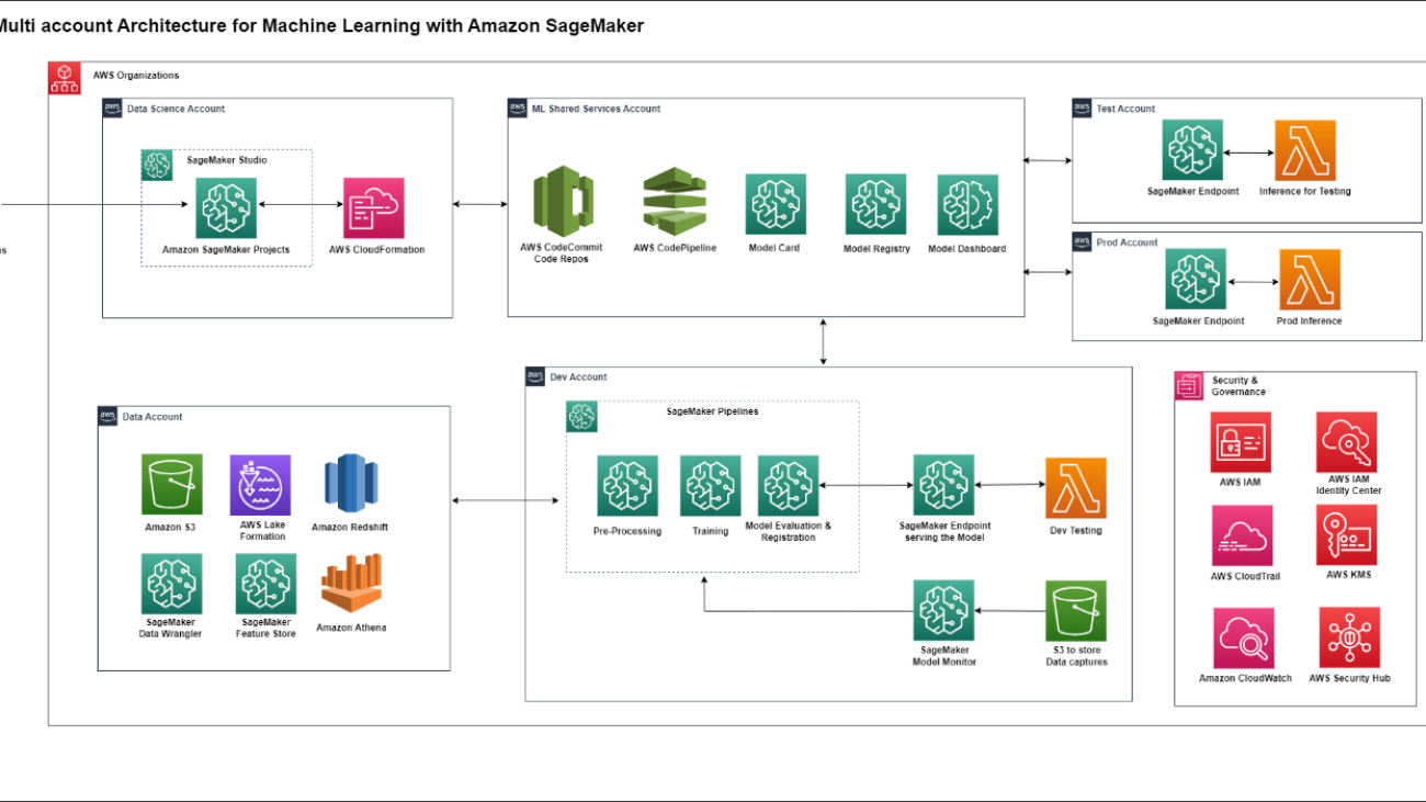
The following diagram illustrates the reference architecture, which has already been discussed in MLOps foundation roadmap for enterprises with Amazon SageMaker.
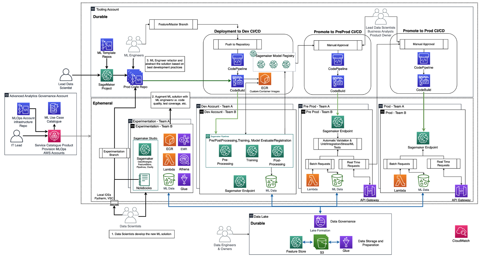
Each business unit has each own set of development (automated model training and building), preproduction (automatic testing), and production (model deployment and serving) accounts to productionize ML use cases, which retrieve data from a centralized or decentralized data lake or data mesh, respectively. All the produced models and code automation are stored in a centralized tooling account using the capability of a model registry. The infrastructure code for all these accounts is versioned in a shared service account (advanced analytics governance account) that the platform team can abstract, templatize, maintain, and reuse for the onboarding to the MLOps platform of every new team.
Generative AI definitions and differences to MLOps
In classic ML, the preceding combination of people, processes, and technology can help you productize your ML use cases. However, in generative AI, the nature of the use cases requires either an extension of those capabilities or new capabilities. One of these new notions is the foundation model (FM). They are called as such because they can be used to create a wide range of other AI models, as illustrated in the following figure.

FM have been trained based on terabytes of data and have hundreds of billions of parameters to be able to predict the next best answer based on three main categories of generative AI use cases:
- Text-to-text – The FMs (LLMs) have been trained based on unlabeled data (such as free text) and are able to predict the next best word or sequence of words (paragraphs or long essays). Main use cases are around human-like chatbots, summarization, or other content creation such as programming code.
- Text-to-image – Labeled data, such as pairs of <text, image>, has been used to train FMs, which are able to predict the best combination of pixels. Example use cases are clothing design generation or imaginary personalized images.
- Text-to-audio or video – Both labeled and unlabeled data can be used for FM training. One main generative AI use case example is music composition.
To productionize those generative AI use cases, we need to borrow and extend the MLOps domain to include the following:
- FM operations (FMOps) – This can productionize generative AI solutions, including any use case type
- LLM operations (LLMOps) – This is a subset of FMOps focusing on productionizing LLM-based solutions, such as text-to-text
The following figure illustrates the overlap of these use cases.
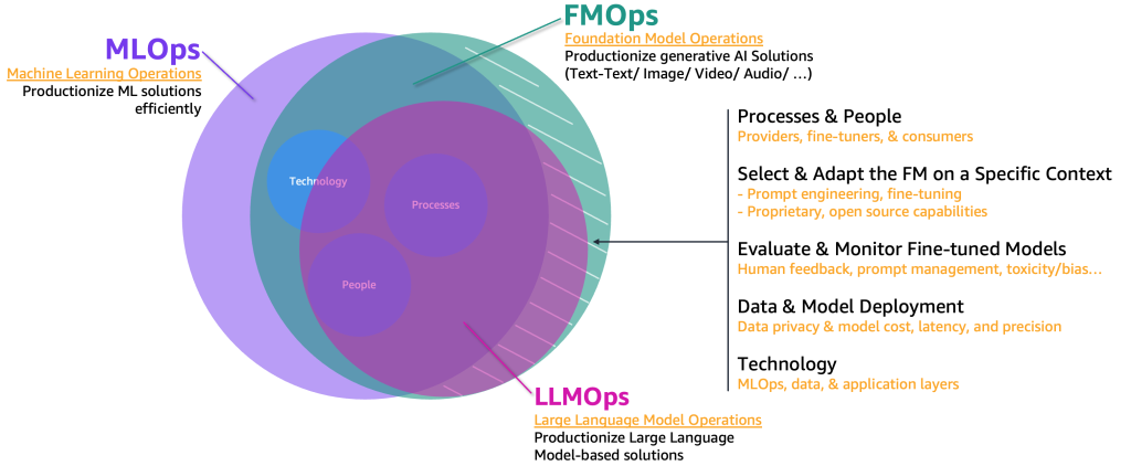
Compared to classic ML and MLOps, FMOps and LLMOps defer based on four main categories that we cover in the following sections: people and process, selection and adaptation of FM, evaluation and monitoring of FM, data privacy and model deployment, and technology needs. We will cover monitoring in a separate post.
Operationalization journey per generative AI user type
To simplify the description of the processes, we need to categorize the main generative AI user types, as shown in the following figure.
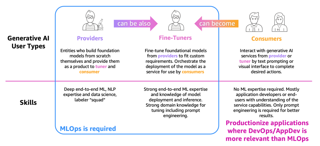
The user types are as follows:
- Providers – Users who build FMs from scratch and provide them as a product to other users (fine-tuner and consumer). They have deep end-to-end ML and natural language processing (NLP) expertise and data science skills, and massive data labeler and editor teams.
- Fine-tuners – Users who retrain (fine-tune) FMs from providers to fit custom requirements. They orchestrate the deployment of the model as a service for use by consumers. These users need strong end-to-end ML and data science expertise and knowledge of model deployment and inference. Strong domain knowledge for tuning, including prompt engineering, is required as well.
- Consumers – Users who interact with generative AI services from providers or fine-tuners by text prompting or a visual interface to complete desired actions. No ML expertise is required but, mostly, application developers or end-users with understanding of the service capabilities. Only prompt engineering is necessary for better results.
As per the definition and the required ML expertise, MLOps is required mostly for providers and fine-tuners, while consumers can use application productionization principles, such as DevOps and AppDev to create the generative AI applications. Furthermore, we have observed a movement among the user types, where providers might become fine-tuners to support use cases based on a specific vertical (such as the financial sector) or consumers might become fine-tuners to achieve more accurate results. But let’s observe the main processes per user type.
The journey of consumers
The following figure illustrates the consumer journey.
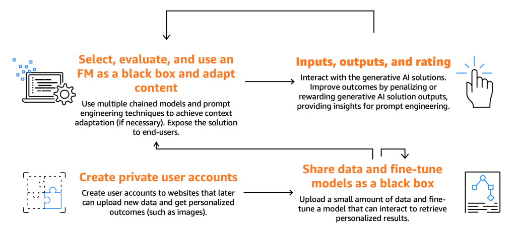
As previously mentioned, consumers are required to select, test, and use an FM, interacting with it by providing specific inputs, otherwise known as prompts. Prompts, in the context of computer programming and AI, refer to the input that is given to a model or system to generate a response. This can be in the form of a text, command, or a question, which the system uses to process and generate an output. The output generated by the FM can then be utilized by end-users, who should also be able to rate these outputs to enhance the model’s future responses.
Beyond these fundamental processes, we’ve noticed consumers expressing a desire to fine-tune a model by harnessing the functionality offered by fine-tuners. Take, for instance, a website that generates images. Here, end-users can set up private accounts, upload personal photos, and subsequently generate content related to those images (for example, generating an image depicting the end-user on a motorbike wielding a sword or located in an exotic location). In this scenario, the generative AI application, designed by the consumer, must interact with the fine-tuner backend via APIs to deliver this functionality to the end-users.
However, before we delve into that, let’s first concentrate on the journey of model selection, testing, usage, input and output interaction, and rating, as shown in the following figure.
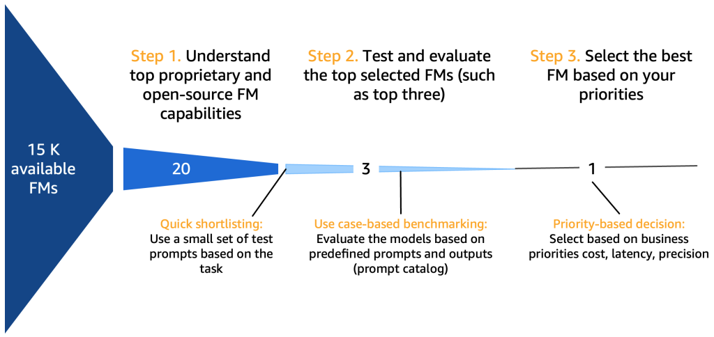
*15K available FM reference
Step 1. Understand top FM capabilities
There are many dimensions that need to be considered when selecting foundation models, depending on the use case, the data available, regulations, and so on. A good checklist, although not comprehensive, might be the following:
- Proprietary or open-source FM – Proprietary models often come at a financial cost, but they typically offer better performance (in terms of quality of the generated text or image), often being developed and maintained by dedicated teams of model providers who ensure optimal performance and reliability. On the other hand, we also see adoption of open-source models that, other than being free, offer additional benefits of being accessible and flexible (for example, every open-source model is fine-tunable). An example of a proprietary model is Anthropic’s Claude model, and an example of a high performing open-source model is Falcon-40B, as of July 2023.
- Commercial license – Licensing considerations are crucial when deciding on an FM. It’s important to note that some models are open-source but can’t be used for commercial purposes, due to licensing restrictions or conditions. The differences can be subtle: The newly released xgen-7b-8k-base model, for example, is open source and commercially usable (Apache-2.0 license), whereas the instruction fine-tuned version of the model xgen-7b-8k-inst is only released for research purposes only. When selecting an FM for a commercial application, it’s essential to verify the license agreement, understand its limitations, and ensure it aligns with the intended use of the project.
- Parameters – The number of parameters, which consist of the weights and biases in the neural network, is another key factor. More parameters generally means a more complex and potentially powerful model, because it can capture more intricate patterns and correlations in the data. However, the trade-off is that it requires more computational resources and, therefore, costs more to run. Additionally, we do see a trend towards smaller models, especially in the open-source space (models ranging from 7–40 billion) that perform well, especially, when fine-tuned.
- Speed – The speed of a model is influenced by its size. Larger models tend to process data slower (higher latency) due to the increased computational complexity. Therefore, it’s crucial to balance the need for a model with high predictive power (often larger models) with the practical requirements for speed, especially in applications, like chat bots, that demand real-time or near-real-time responses.
- Context window size (number of tokens) – The context window, defined by the maximum number of tokens that can be input or output per prompt, is crucial in determining how much context the model can consider at a time (a token roughly translates to 0.75 words for English). Models with larger context windows can understand and generate longer sequences of text, which can be useful for tasks involving longer conversations or documents.
- Training dataset – It’s also important to understand what kind of data the FM was trained on. Some models may be trained on diverse text datasets like internet data, coding scripts, instructions, or human feedback. Others may also be trained on multimodal datasets, like combinations of text and image data. This can influence the model’s suitability for different tasks. In addition, an organization might have copyright concerns depending on the exact sources a model has been trained on—therefore, it’s mandatory to inspect the training dataset closely.
- Quality – The quality of an FM can vary based on its type (proprietary vs. open source), size, and what it was trained on. Quality is context-dependent, meaning what is considered high-quality for one application might not be for another. For example, a model trained on internet data might be considered high quality for generating conversational text, but less so for technical or specialized tasks.
- Fine-tunable – The ability to fine-tune an FM by adjusting its model weights or layers can be a crucial factor. Fine-tuning allows for the model to better adapt to the specific context of the application, improving performance on the specific task at hand. However, fine-tuning requires additional computational resources and technical expertise, and not all models support this feature. Open-source models are (in general) always fine-tunable because the model artifacts are available for downloading and the users are able to extend and use them at will. Proprietary models might sometimes offer the option of fine-tuning.
- Existing customer skills – The selection of an FM can also be influenced by the skills and familiarity of the customer or the development team. If an organization has no AI/ML experts in their team, then an API service might be better suited for them. Also, if a team has extensive experience with a specific FM, it might be more efficient to continue using it rather than investing time and resources to learn and adapt to a new one.
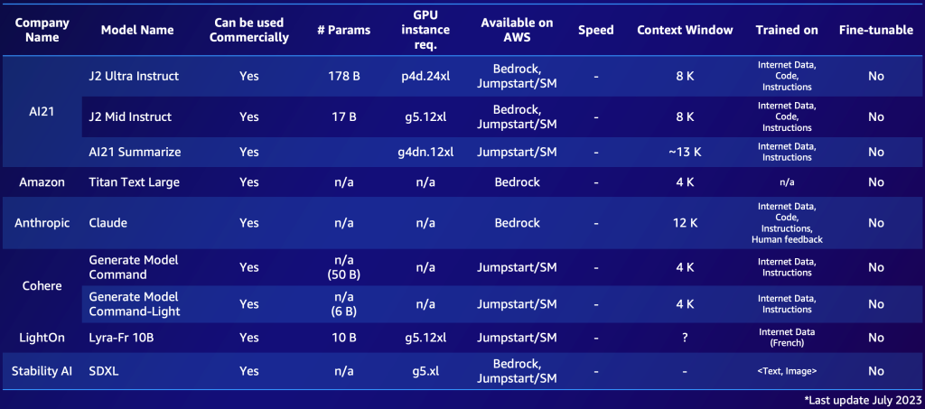
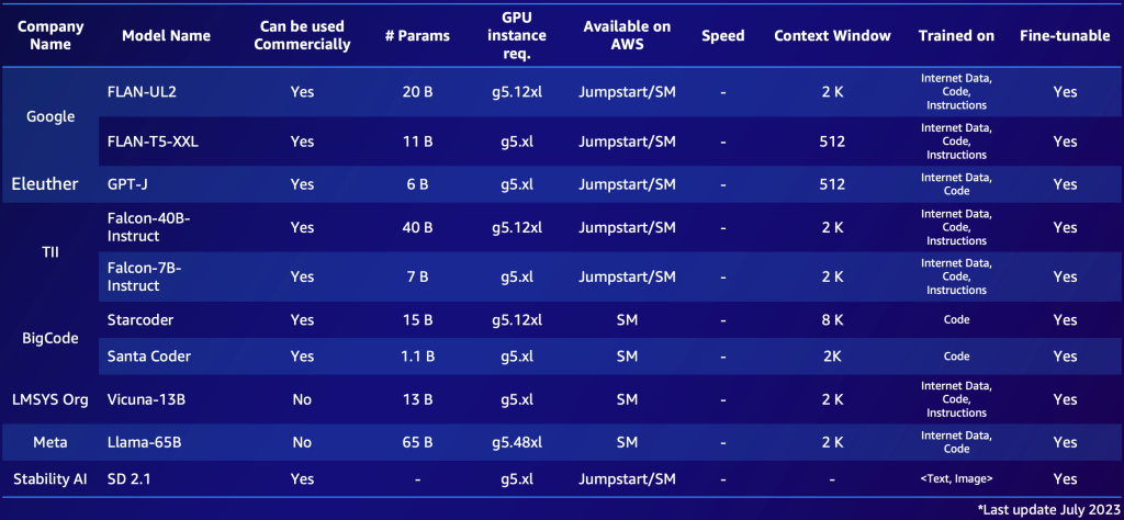
The following is an example of two shortlists, one for proprietary models and one for open-source models. You might compile similar tables based on your specific needs to get a quick overview of the available options. Note that the performance and parameters of those models change rapidly and might be outdated by the time of reading, while other capabilities might be important for specific customers, such as the supported language.
The following is an example of notable proprietary FMs available in AWS (July 2023).
The following is an example of notable open-source FM available in AWS (July 2023).
After you have compiled an overview of 10–20 potential candidate models, it becomes necessary to further refine this shortlist. In this section, we propose a swift mechanism that will yield two or three viable final models as candidates for the next round.
The following diagram illustrates the initial shortlisting process.
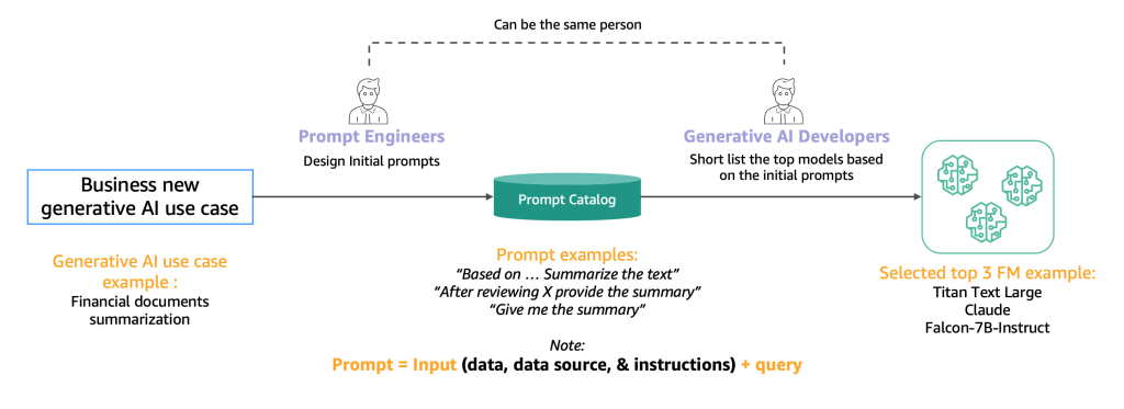
Typically, prompt engineers, who are experts in creating high-quality prompts that allow AI models to understand and process user inputs, experiment with various methods to perform the same task (such as summarization) on a model. We suggest that these prompts are not created on the fly, but are systematically extracted from a prompt catalog. This prompt catalog is a central location for storing prompts to avoid replications, enable version control, and share prompts within the team to ensure consistency between different prompt testers in the different development stages, which we introduce in the next section. This prompt catalog is analogous to a Git repository of a feature store. The generative AI developer, who could potentially be the same person as the prompt engineer, then needs to evaluate the output to determine if it would be suitable for the generative AI application they are seeking to develop.
Step 2. Test and evaluate the top FM
After the shortlist is reduced to approximately three FMs, we recommend an evaluation step to further test the FMs’ capabilities and suitability for the use case. Depending on the availability and nature of evaluation data, we suggest different methods, as illustrated in the following figure.
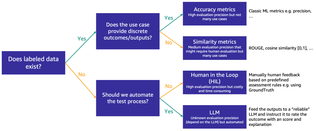
The method to use first depends on whether you have labeled test data or not.
If you have labeled data, you can use it to conduct a model evaluation, as we do with the traditional ML models (input some samples and compare the output with the labels). Depending on whether the test data has discrete labels (such as positive, negative, or neutral sentiment analysis) or is unstructured text (such as summarization), we propose different methods for evaluation:
- Accuracy metrics – In case of discrete outputs (such as sentiment analysis), we can use standard accuracy metrics such as precision, recall, and F1 score
- Similarity metrics – If the output is unstructured (such as a summary), we suggest similarity metrics like ROUGE and cosine similarity
Some use cases don’t lend themselves to having one true answer (for example, “Create a short children’s story for my 5-year-old daughter”). In such cases, it becomes more challenging to evaluate the models because you don’t have labeled test data. We propose two approaches, depending on the importance of human review of the model versus automated evaluation:
- Human-in-the-Loop (HIL) – In this case, a team of prompt testers will review the responses from a model. Depending on how critical the application is, the prompt testers might review 100% of the model outputs or just a sample.
- LLM-powered evaluation – In this scenario, the prompt testers are replaced by an LLM, ideally one that is more powerful (although perhaps slower and most costly) than the ones being tested. The LLM will review all model-generated responses and score them. This method may result in lower quality, but it’s a cheaper and faster evaluation option that might provide a good initial gauge on the models’ performance.
For example, we can use the following example prompt to an LLM, which includes the input query, the LLM response, and instructions: “We would like to request your feedback on the performance of an AI assistant in response to the user question displayed above. Please rate the helpfulness, relevance, accuracy, level of details of the assistant’s response. The assistant shall receive an overall score on a scale of 1 to 10, where a higher score indicates better overall performance.”
This prompt will be sent to another LLM (the EvalLLM) for evaluation. The following is an example where the response of the Falcon-40B model has been evaluated by an EvalLLM (in this case Claude). We use the question “What if the Suez Canal had never been constructed?” The response is as follows:
Question: What if the Suez Canal had never been constructed?
falcon-40b-instruct
If the Suez Canal had never been constructed, ships would have to travel around Africa to navigate between the Mediterranean and the Red Sea. This would add significant time and distance to the voyage, making it less efficient and more expensive. Additionally, without the Suez Canal, many countries in the Middle East and North Africa would have been much less connected to the rest of the world, hindering economic and cultural development.
Review (Score: 9/10)
The assistant’s response is highly relevant, accurate, and detailed. It provides an excellent answer to the user’s hypothetical question about the non-existence of the Suez Canal. The assistant correctly points out the implications on maritime travel and the economic and cultural impact on the Middle East and North Africa. However, it could have further elaborated on the geopolitical implications or the impact on global trade patterns for a more comprehensive response.
The following figure illustrates the end-to-end evaluation process example.
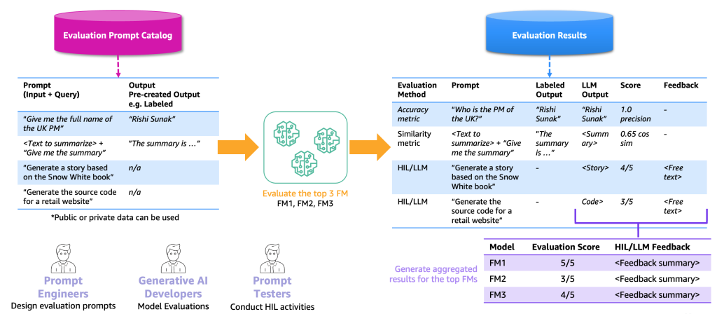
Based on this example, to perform evaluation, we need to provide the example prompts, which we store in the prompt catalog, and an evaluation labeled or unlabeled dataset based on our specific applications. For example, with a labeled evaluation dataset, we can provide prompts (input and query) such as “Give me the full name of the UK PM in 2023” and outputs and answers, such as “Rishi Sunak.” With an unlabeled dataset, we provide just the question or instruction, such as “Generate the source code for a retail website.” We call the combination of prompt catalog and evaluation dataset the evaluation prompt catalog. The reason that we differentiate the prompt catalog and evaluation prompt catalog is because the latter is dedicated to a specific use case instead of generic prompts and instructions (such as question answering) that the prompt catalog contains.
With this evaluation prompt catalog, the next step is to feed the evaluation prompts to the top FMs. The result is an evaluation result dataset that contains the prompts, outputs of each FM, and the labeled output together with a score (if it exists). In the case of an unlabeled evaluation prompt catalog, there is an additional step for an HIL or LLM to review the results and provide a score and feedback (as we described earlier). The final outcome will be aggregated results that combine the scores of all the outputs (calculate the average precision or human rating) and allow the users to benchmark the quality of the models.
After the evaluation results have been collected, we propose choosing a model based on several dimensions. These typically come down to factors such as precision, speed, and cost. The following figure shows an example.
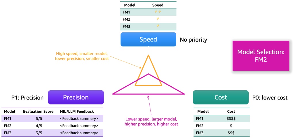
Each model will possess strengths and certain trade-offs along these dimensions. Depending on the use case, we should assign varying priorities to these dimensions. In the preceding example, we elected to prioritize cost as the most important factor, followed by precision, and then speed. Even though it’s slower and not as efficient as FM1, it remains sufficiently effective and significantly cheaper to host. Consequently, we might select FM2 as the top choice.
Step 3. Develop the generative AI application backend and frontend
At this point, the generative AI developers have selected the right FM for the specific application together with the help of prompt engineers and testers. The next step is to start developing the generative AI application. We have separated the development of the generative AI application into two layers, a backend and front end, as shown in the following figure.
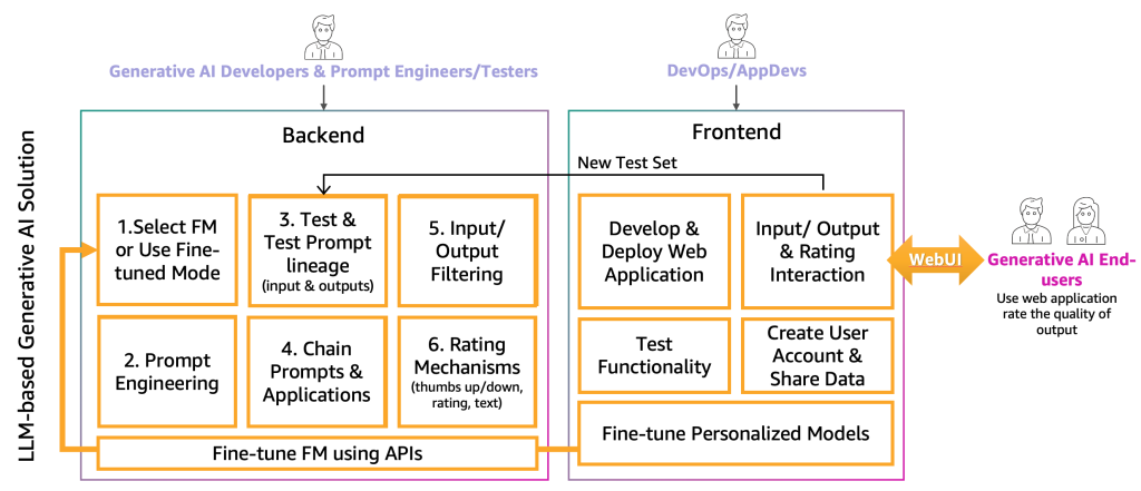
On the backend, the generative AI developers incorporate the selected FM into the solutions and work together with the prompt engineers to create the automation to transform the end-user input to appropriate FM prompts. The prompt testers create the necessary entries to the prompt catalog for automatic or manual (HIL or LLM) testing. Then, the generative AI developers create the prompt chaining and application mechanism to provide the final output. Prompt chaining, in this context, is a technique to create more dynamic and contextually-aware LLM applications. It works by breaking down a complex task into a series of smaller, more manageable sub-tasks. For example, if we ask an LLM the question “Where was the prime minister of the UK born and how far is that place from London,” the task can be broken down into individual prompts, where a prompt might be built based on the answer of a previous prompt evaluation, such as “Who is the prime minister of the UK,” “What is their birthplace,” and “How far is that place from London?” To ensure a certain input and output quality, the generative AI developers also need to create the mechanism to monitor and filter the end-user inputs and application outputs. If, for example, the LLM application is supposed to avoid toxic requests and responses, they could apply a toxicity detector for input and output and filter those out. Lastly, they need to provide a rating mechanism, which will support the augmentation of the evaluation prompt catalog with good and bad examples. A more detailed representation of those mechanisms will be presented in future posts.
To provide the functionality to the generative AI end-user, the development of a frontend website that interacts with the backend is necessary. Therefore, DevOps and AppDevs (application developers on the cloud) personas need to follow best development practices to implement the functionality of input/output and rating.
In addition to this basic functionality, the frontend and backend need to incorporate the feature of creating personal user accounts, uploading data, initiating fine-tuning as a black box, and using the personalized model instead of the basic FM. The productionization of a generative AI application is similar with a normal application. The following figure depicts an example architecture.
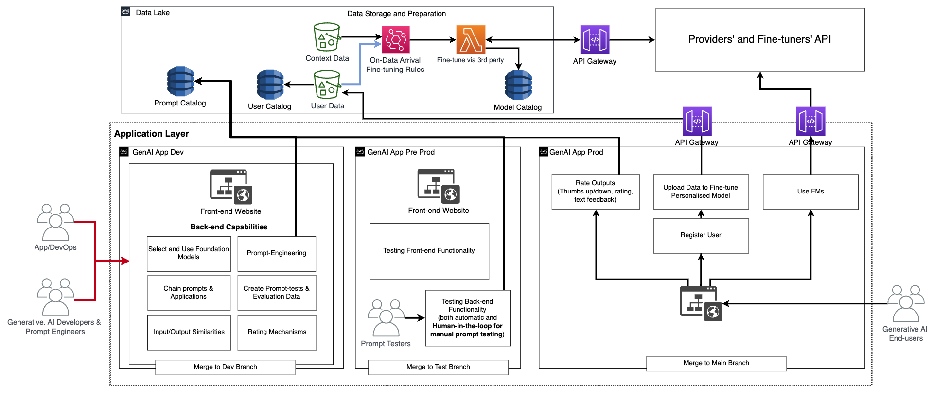
In this architecture, the generative AI developers, prompt engineers, and DevOps or AppDevs create and test the application manually by deploying it via CI/CD to a development environment (generative AI App Dev in the preceding figure) using dedicated code repositories and merging with the dev branch. At this stage, the generative AI developers will use the corresponding FM by calling the API as has been provided by the FM providers of fine-tuners. Then, to test the application extensively, they need to promote the code to the test branch, which will trigger the deployment via CI/CD to the preproduction environment (generative AI App Pre-prod). At this environment, the prompt testers need to try a large amount of prompt combinations and review the results. The combination of prompts, outputs, and review need to be moved to the evaluation prompt catalog to automate the testing process in the future. After this extensive test, the last step is to promote the generative AI application to production via CI/CD by merging with the main branch (generative AI App Prod). Note that all the data, including the prompt catalog, evaluation data and results, end-user data and metadata, and fine-tuned model metadata, need to be stored in the data lake or data mesh layer. The CI/CD pipelines and repositories need to be stored in a separate tooling account (similar to the one described for MLOps).
The journey of providers
FM providers need to train FMs, such as deep learning models. For them, the end-to-end MLOps lifecycle and infrastructure is necessary. Additions are required in historical data preparation, model evaluation, and monitoring. The following figure illustrates their journey.
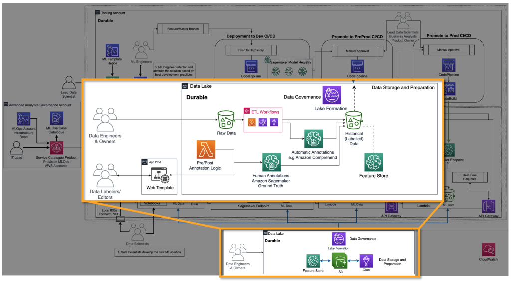
In classic ML, the historical data is most often created by feeding the ground truth via ETL pipelines. For example, in a churn prediction use case, an automation updates a database table based on the new status of a customer to churn/not churn automatically. In the case of FMs, they need either billions of labeled or unlabeled data points. In text-to-image use cases, a team of data labelers need to label <text, image> pairs manually. This is an expensive exercise requiring a large number of people resources. Amazon SageMaker Ground Truth Plus can provide a team of labelers to perform this activity for you. For some use cases, this process can be also partially automated, for example by using CLIP-like models. In the case of an LLM, such as text-to-text, the data is unlabeled. However, they need to be prepared and follow the format of the existing historical unlabeled data. Therefore, data editors are needed to perform necessary data preparation and ensure consistency.
With the historical data prepared, the next step is the training and productionization of the model. Note that the same evaluation techniques as we described for consumers can be used.
The journey of fine-tuners
Fine-tuners aim to adapt an existing FM to their specific context. For example, an FM model can summarize a general-purpose text but not a financial report accurately or can’t generate source code for a non-common programming language. In those cases, the fine-tuners need to label data, fine-tune a model by running a training job, deploy the model, test it based on the consumer processes, and monitor the model. The following diagram illustrates this process.
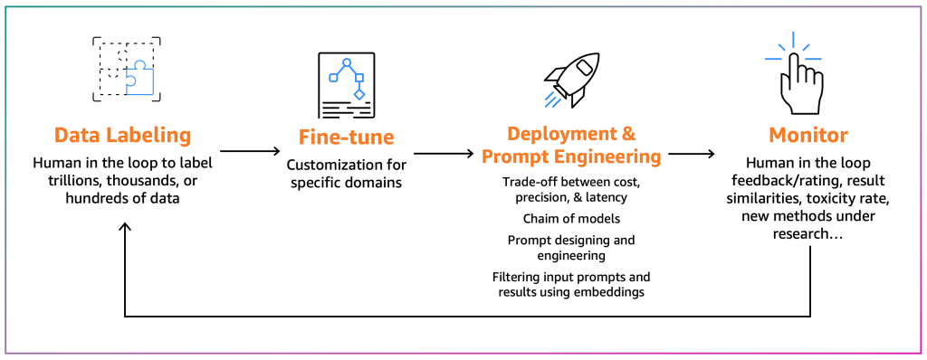
For the time being, there are two fine-tuning mechanisms:
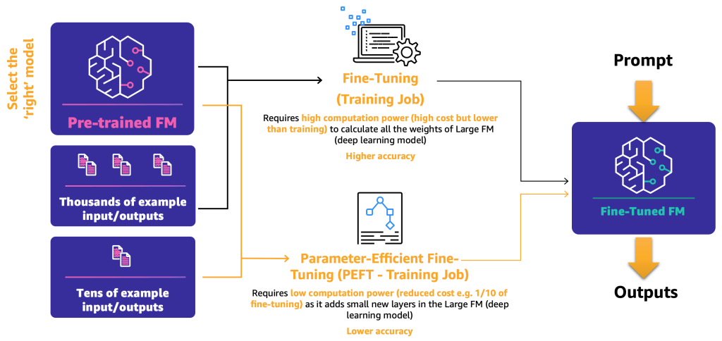
- Fine-tuning – By using an FM and labeled data, a training job recalculates the weights and biases of the deep learning model layers. This process can be computationally intensive and requires a representative amount of data but can generate accurate results.
- Parameter-efficient fine-tuning (PEFT) – Instead of recalculating all the weights and biases, researchers have shown that by adding additional small layers to the deep learning models, they can achieve satisfactory results (for example, LoRA). PEFT requires lower computational power than deep fine-tuning and a training job with less input data. The drawback is potential lower accuracy.
The following diagram illustrates these mechanisms.
Now that we have defined the two main fine-tuning methods, the next step is to determine how we can deploy and use the open-source and proprietary FM.
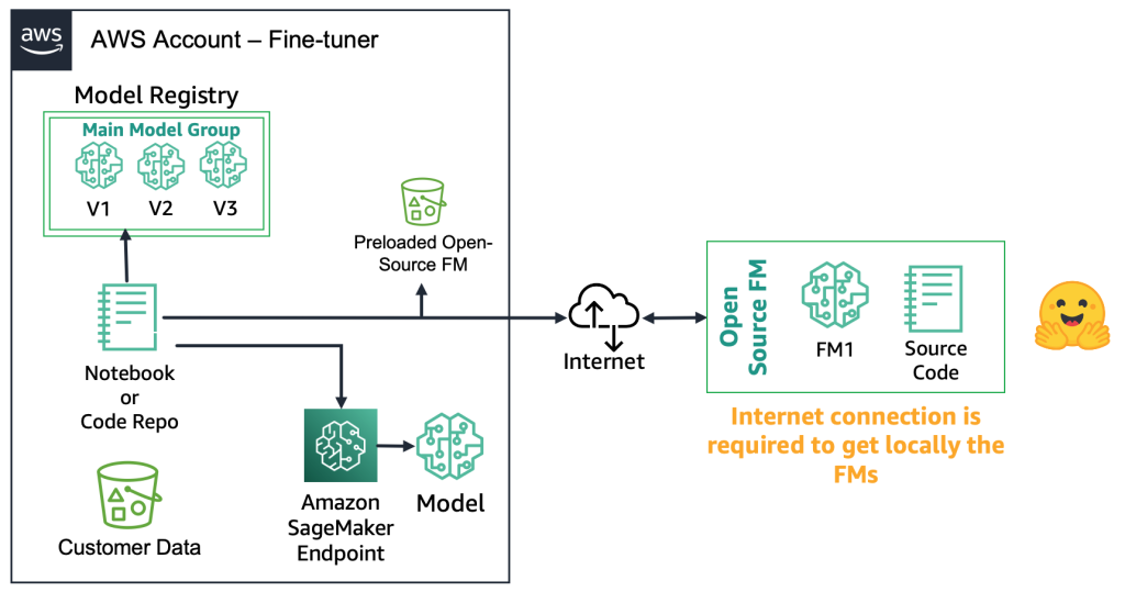
With open-source FMs, the fine-tuners can download the model artifact and the source code from the web, for example, by using the Hugging Face Model Hub. This gives you the flexibility to deep fine-tune the model, store it to a local model registry, and deploy it to an Amazon SageMaker endpoint. This process requires an internet connection. To support more secure environments (such as for customers in the financial sector), you can download the model on premises, run all the necessary security checks, and upload them to a local bucket on an AWS account. Then, the fine-tuners use the FM from the local bucket without an internet connection. This ensures data privacy, and the data doesn’t travel over the internet. The following diagram illustrates this method.
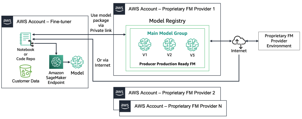
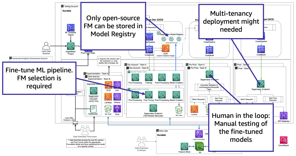
With proprietary FMs, the deployment process is different because the fine-tuners don’t have access to the model artifact or source code. The models are stored in proprietary FM provider AWS accounts and model registries. To deploy such a model to a SageMaker endpoint, the fine-tuners can request only the model package that will be deployed directly to an endpoint. This process requires customer data to be used in the proprietary FM providers’ accounts, which raises questions regarding customer-sensitive data being used in a remote account to perform fine-tuning, and models being hosted in a model registry that is shared among multiple customers. This leads to a multi-tenancy problem that becomes more challenging if the proprietary FM providers need to serve these models. If the fine-tuners use Amazon Bedrock, these challenges are resolved—the data doesn’t travel over the internet and the FM providers don’t have access to fine-tuners’ data. The same challenges hold for the open-source models if the fine-tuners want to serve models from multiple customers, such as the example we gave earlier with the website that thousands of customers will upload personalized images to. However, these scenarios can be considered controllable because only the fine-tuner is involved. The following diagram illustrates this method.
From a technology perspective, the architecture that a fine-tuner needs to support is like the one for MLOps (see the following figure). The fine-tuning needs to be conducted in dev by creating ML pipelines, such as using Amazon SageMaker Pipelines; performing preprocessing, fine-tuning (training job), and postprocessing; and sending the fine-tuned models to a local model registry in the case of an open-source FM (otherwise, the new model will be stored to the proprietary FM provide environment). Then, in pre-production, we need to test the model as we describe for the consumers’ scenario. Finally, the model will be served and monitored in prod. Note that the current (fine-tuned) FM requires GPU instance endpoints. If we need to deploy each fine-tuned model to a separate endpoint, this might increase the cost in the case of hundreds of models. Therefore, we need to use multi-model endpoints and resolve the multi-tenancy challenge.
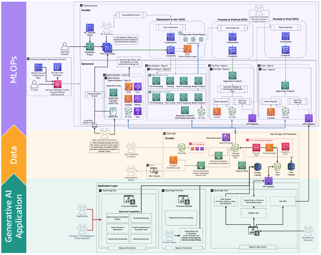
The fine-tuners adapt an FM model based on a specific context to use it for their business purpose. That means that most of the time, the fine-tuners are also consumers required to support all the layers, as we described in the previous sections, including generative AI application development, data lake and data mesh, and MLOps.
The following figure illustrates the complete FM fine-tuning lifecycle that the fine-tuners need to provide the generative AI end-user.
The following figure illustrates the key steps.
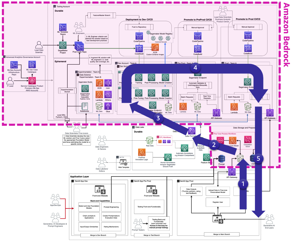
The key steps are the following:
- The end-user creates a personal account and uploads private data.
- The data is stored in the data lake and is preprocessed to follow the format that the FM expects.
- This triggers a fine-tuning ML pipeline that adds the model to the model registry,
- From there, either the model is deployed to production with minimum testing or the model pushes extensive testing with HIL and manual approval gates.
- The fine-tuned model is made available for end-users.
Because this infrastructure is complex for non-enterprise customers, AWS released Amazon Bedrock to offload the effort of creating such architectures and bringing fine-tuned FMs closer to production.
FMOps and LLMOps personas and processes differentiators
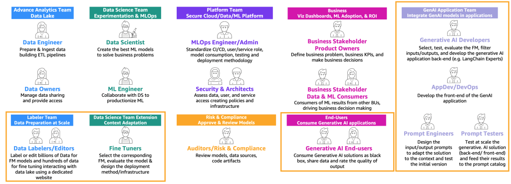
Based on the preceding user type journeys (consumer, producer, and fine-tuner), new personas with specific skills are required, as illustrated in the following figure.
The new personas are as follows:
- Data labelers and editors – These users label data, such as <text, image> pairs, or prepare unlabeled data, such as free text, and extend the advanced analytics team and data lake environments.
- Fine-tuners – These users have deep knowledge on FMs and know to tune them, extending the data science team that will focus on classic ML.
- Generative AI developers – They have deep knowledge on selecting FMs, chaining prompts and applications, and filtering input and outputs. They belong a new team—the generative AI application team.
- Prompt engineers – These users design the input and output prompts to adapt the solution to the context and test and create the initial version of prompt catalog. Their team is the generative AI application team.
- Prompt testers – They test at scale the generative AI solution (backend and frontend) and feed their results to augment the prompt catalog and evaluation dataset. Their team is the generative AI application team.
- AppDev and DevOps – They develop the front end (such as a website) of the generative AI application. Their team is the generative AI application team.
- Generative AI end-users – These users consume generative AI applications as black boxes, share data, and rate the quality of the output.
The extended version of the MLOps process map to incorporate generative AI can be illustrated with the following figure.
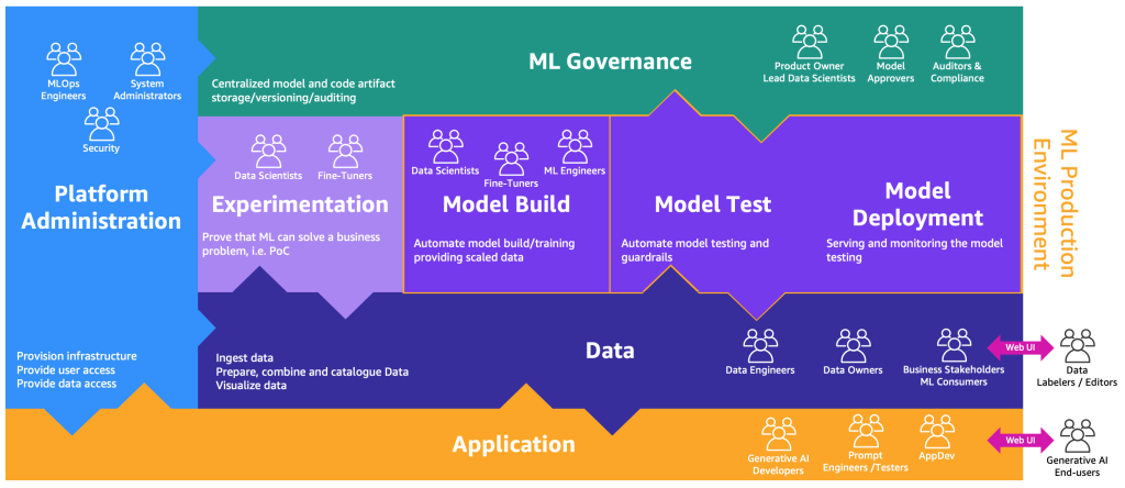
A new application layer is the environment where generative AI developers, prompt engineers, and testers, and AppDevs created the backend and front end of generative AI applications. The generative AI end-users interact with the generative AI applications front end via the internet (such as a web UI). On the other side, data labelers and editors need to preprocess the data without accessing the backend of the data lake or data mesh. Therefore, a web UI (website) with an editor is necessary for interacting securely with the data. SageMaker Ground Truth provides this functionality out of the box.
Conclusion
MLOps can help us productionize ML models efficiently. However, to operationalize generative AI applications, you need additional skills, processes, and technologies, leading to FMOps and LLMOps. In this post, we defined the main concepts of FMOps and LLMOps and described the key differentiators compared to MLOps capabilities in terms of people, processes, technology, FM model selection, and evaluation. Furthermore, we illustrated the thought process of a generative AI developer and the development lifecycle of a generative AI application.
In the future, we will focus on providing solutions per the domain we discussed, and will provide more details on how to integrate FM monitoring (such as toxicity, bias, and hallucination) and third-party or private data source architectural patterns, such as Retrieval Augmented Generation (RAG), into FMOps/LLMOps.
To learn more, refer to MLOps foundation roadmap for enterprises with Amazon SageMaker and try out the end-to-end solution in Implementing MLOps practices with Amazon SageMaker JumpStart pre-trained models.
If you have any comments or questions, please leave them in the comments section.
About the Authors
 Dr. Sokratis Kartakis is a Senior Machine Learning and Operations Specialist Solutions Architect for Amazon Web Services. Sokratis focuses on enabling enterprise customers to industrialize their Machine Learning (ML) solutions by exploiting AWS services and shaping their operating model, i.e. MLOps foundation, and transformation roadmap leveraging best development practices. He has spent 15+ years on inventing, designing, leading, and implementing innovative end-to-end production-level ML and Internet of Things (IoT) solutions in the domains of energy, retail, health, finance/banking, motorsports etc. Sokratis likes to spend his spare time with family and friends, or riding motorbikes.
 Heiko Hotz is a Senior Solutions Architect for AI & Machine Learning with a special focus on natural language processing, large language models, and generative AI. Prior to this role, he was the Head of Data Science for Amazon’s EU Customer Service. Heiko helps our customers be successful in their AI/ML journey on AWS and has worked with organizations in many industries, including insurance, financial services, media and entertainment, healthcare, utilities, and manufacturing. In his spare time, Heiko travels as much as possible.
Read More


 Praveen Edem is a Senior Solutions Architect at Amazon Web Services. He works with major financial services customers, architecting and modernizing their critical large-scale applications while adopting AWS services. He specializes in serverless and container-based workloads. He has over 20 years of IT experience in application development and software architecture.
 Manjula Nagineni is a Senior Solutions Architect with AWS based in New York. She works with major financial service institutions, architecting and modernizing their large-scale applications while adopting AWS Cloud services. She is passionate about designing big data workloads cloud-natively. She has over 20 years of IT experience in software development, analytics, and architecture across multiple domains such as finance, manufacturing, and telecom.
 Omkar Phadtare is a Software Development Engineer at Amazon Web Services, with a deep-rooted passion for cloud computing. Leveraging his technical expertise and strong understanding of the domain, he designs, develops, and implements cutting-edge, highly scalable, and resilient cloud-based solutions for a diverse range of modern businesses and organizations.
 Vijai Gandikota is a Senior Product Manager for Amazon Kendra at Amazon Web Services, responsible for launching Amazon Kendra connectors, Principal Store, Search Analytics Dashboard, and other features of Amazon Kendra. He has over 20 years of experience in designing, developing, and launching products in AI and analytics.


 Dr. Vivek Madan is an Applied Scientist with the Amazon SageMaker JumpStart team. He got his PhD from University of Illinois at Urbana-Champaign and was a Post Doctoral Researcher at Georgia Tech. He is an active researcher in machine learning and algorithm design and has published papers in EMNLP, ICLR, COLT, FOCS, and SODA conferences.
 Dr. Farooq Sabir is a Senior Artificial Intelligence and Machine Learning Specialist Solutions Architect at AWS. He holds PhD and MS degrees in Electrical Engineering from the University of Texas at Austin and an MS in Computer Science from Georgia Institute of Technology. He has over 15 years of work experience and also likes to teach and mentor college students. At AWS, he helps customers formulate and solve their business problems in data science, machine learning, computer vision, artificial intelligence, numerical optimization, and related domains. Based in Dallas, Texas, he and his family love to travel and go on long road trips.
 Dr. Ashish Khetan is a Senior Applied Scientist with Amazon SageMaker JumpStart and helps develop machine learning algorithms. He got his PhD from University of Illinois Urbana-Champaign. He is an active researcher in machine learning and statistical inference, and has published many papers in NeurIPS, ICML, ICLR, JMLR, ACL, and EMNLP conferences.


 James Wu is a Senior AI/ML Specialist Solution Architect at AWS. helping customers design and build AI/ML solutions. James’s work covers a wide range of ML use cases, with a primary interest in computer vision, deep learning, and scaling ML across the enterprise. Prior to joining AWS, James was an architect, developer, and technology leader for over 10 years, including 6 years in engineering and 4 years in marketing & advertising industries.
 Li Ning is a senior software engineer at AWS with a specialization in building large-scale AI solutions. As a tech lead for TorchServe, a project jointly developed by AWS and Meta, her passion lies in leveraging PyTorch and AWS SageMaker to help customers embrace AI for the greater good. Outside of her professional endeavors, Li enjoys swimming, traveling, following the latest advancements in technology, and spending quality time with her family.
 Ankith Gunapal is an AI Partner Engineer at Meta (PyTorch). He is passionate about model optimization and model serving, with experience ranging from RTL verification, embedded software, computer vision, to PyTorch. He holds a Master’s in Data Science and a Master’s in Telecommunications. Outside of work, Ankith is also an electronic dance music producer.
 Saurabh Trikande is a Senior Product Manager for Amazon SageMaker Inference. He is passionate about working with customers and is motivated by the goal of democratizing machine learning. He focuses on core challenges related to deploying complex ML applications, multi-tenant ML models, cost optimizations, and making deployment of deep learning models more accessible. In his spare time, Saurabh enjoys hiking, learning about innovative technologies, following TechCrunch and spending time with his family.
 Subhash Talluri is a Lead AI/ML solutions architect of the Telecom Industry business unit at Amazon Web Services. He’s been leading development of innovative AI/ML solutions for Telecom customers and partners worldwide. He brings interdisciplinary expertise in engineering and computer science to help build scalable, secure, and compliant AI/ML solutions via cloud-optimized architectures on AWS.


 Gordon Wang is a Senior AI/ML Specialist TAM at AWS. He supports strategic customers with AI/ML best practices cross many industries. He is passionate about computer vision, NLP, generative AI, and MLOps. In his spare time, he loves running and hiking.
 Yanwei Cui, PhD, is a Senior Machine Learning Specialist Solutions Architect at AWS. He started machine learning research at IRISA (Research Institute of Computer Science and Random Systems), and has several years of experience building AI-powered industrial applications in computer vision, natural language processing, and online user behavior prediction. At AWS, he shares his domain expertise and helps customers unlock business potentials and drive actionable outcomes with machine learning at scale. Outside of work, he enjoys reading and traveling.
 Melanie Li, PhD, is a Senior AI/ML Specialist TAM at AWS based in Sydney, Australia. She helps enterprise customers build solutions using state-of-the-art AI/ML tools on AWS and provides guidance on architecting and implementing ML solutions with best practices. In her spare time, she loves to explore nature and spend time with family and friends.


 Ravi Patankar is a technical leader for IoT related analytics at Carrier’s Residential HVAC Unit. He formulates analytics problems related to diagnostics and prognostics and provides direction for ML/deep learning-based analytics solutions and architecture.
 Dan Volk is a Data Scientist at the AWS Generative AI Innovation Center. He has ten years of experience in machine learning, deep learning and time-series analysis and holds a Master’s in Data Science from UC Berkeley. He is passionate about transforming complex business challenges into opportunities by leveraging cutting-edge AI technologies.
 Yingwei Yu is an Applied Scientist at AWS Generative AI Innovation Center. He has experience working with several organizations across industries on various proof-of-concepts in machine learning, including NLP, time-series analysis, and generative AI technologies. Yingwei received his PhD in computer science from Texas A&M University.
 Yanxiang Yu is an Applied Scientist at Amazon Web Services, working on the Generative AI Innovation Center. With over 8 years of experience building AI and machine learning models for industrial applications, he specializes in generative AI, computer vision, and time series modeling. His work focuses on finding innovative ways to apply advanced generative techniques to real-world problems.
 Diego Socolinsky is a Senior Applied Science Manager with the AWS Generative AI Innovation Center, where he leads the delivery team for the Eastern US and Latin America regions. He has over twenty years of experience in machine learning and computer vision, and holds a PhD degree in mathematics from The Johns Hopkins University.
 Kexin Ding is a fifth-year Ph.D. candidate in computer science at UNC-Charlotte. Her research focuses on applying deep learning methods for analyzing multi-modal data, including medical image and genomics sequencing data.


 Davide Gallitelli is a Specialist Solutions Architect for AI/ML in the EMEA region. He is based in Brussels and works closely with customers throughout Benelux. He has been a developer since he was very young, starting to code at the age of 7. He started learning AI/ML at university, and has fallen in love with it since then.


 Raghu Ramesha is a Senior ML Solutions Architect with the Amazon SageMaker Service team. He focuses on helping customers build, deploy, and migrate ML production workloads to SageMaker at scale. He specializes in machine learning, AI, and computer vision domains, and holds a master’s degree in Computer Science from UT Dallas. In his free time, he enjoys traveling and photography.
 Abhi Shivaditya is a Senior Solutions Architect at AWS, working with strategic global enterprise organizations to facilitate the adoption of AWS services in areas such as artificial intelligence, distributed computing, networking, and storage. His expertise lies in deep learning in the domains of natural language processing (NLP) and computer vision. Abhi assists customers in deploying high-performance machine learning models efficiently within the AWS ecosystem.
 Alan Tan is a Senior Product Manager with SageMaker, leading efforts on large model inference. He’s passionate about applying machine learning to the area of analytics. Outside of work, he enjoys the outdoors.
 Melanie Li, PhD, is a Senior AI/ML Specialist TAM at AWS based in Sydney, Australia. She helps enterprise customers build solutions using state-of-the-art AI/ML tools on AWS and provides guidance on architecting and implementing ML solutions with best practices. In her spare time, she loves to explore nature and spend time with family and friends.
 Sam Edwards, is a Cloud Engineer (AI/ML) at AWS Sydney specialized in machine learning and Amazon SageMaker. He is passionate about helping customers solve issues related to machine learning workflows and creating new solutions for them. Outside of work, he enjoys playing racquet sports and traveling.
 James Sanders is a Senior Software Engineer at Amazon Web Services. He works on the real-time inference platform for Amazon SageMaker.


 Dr. Sokratis Kartakis is a Senior Machine Learning and Operations Specialist Solutions Architect for Amazon Web Services. Sokratis focuses on enabling enterprise customers to industrialize their Machine Learning (ML) solutions by exploiting AWS services and shaping their operating model, i.e. MLOps foundation, and transformation roadmap leveraging best development practices. He has spent 15+ years on inventing, designing, leading, and implementing innovative end-to-end production-level ML and Internet of Things (IoT) solutions in the domains of energy, retail, health, finance/banking, motorsports etc. Sokratis likes to spend his spare time with family and friends, or riding motorbikes.
 Heiko Hotz is a Senior Solutions Architect for AI & Machine Learning with a special focus on natural language processing, large language models, and generative AI. Prior to this role, he was the Head of Data Science for Amazon’s EU Customer Service. Heiko helps our customers be successful in their AI/ML journey on AWS and has worked with organizations in many industries, including insurance, financial services, media and entertainment, healthcare, utilities, and manufacturing. In his spare time, Heiko travels as much as possible.


 Ram Vittal is a Principal ML Solutions Architect at AWS. He has over 20 years of experience architecting and building distributed, hybrid, and cloud applications. He is passionate about building secure and scalable AI/ML and big data solutions to help enterprise customers with their cloud adoption and optimization journey to improve their business outcomes. In his spare time, he rides his motorcycle and walks with his 2-year-old sheep-a-doodle!