Posts in category: Amazon AWS

Generative AI models have been experiencing rapid growth in recent months due to its impressive capabilities in creating realistic text, images, code, and audio. Among these models, Stable Diffusion models stand out for their unique strength in creating high-quality images based on text prompts. Stable Diffusion can generate a wide variety of high-quality images, including realistic portraits, landscapes, and even abstract art. And, like other generative AI models, Stable Diffusion models require powerful computing to provide low-latency inference.

In this post, we show how you can run Stable Diffusion models and achieve high performance at the lowest cost in Amazon Elastic Compute Cloud (Amazon EC2) using Amazon EC2 Inf2 instances powered by AWS Inferentia2. We look at the architecture of a Stable Diffusion model and walk through the steps of compiling a Stable Diffusion model using AWS Neuron and deploying it to an Inf2 instance. We also discuss the optimizations that the Neuron SDK automatically makes to improve performance. You can run both Stable Diffusion 2.1 and 1.5 versions on AWS Inferentia2 cost-effectively. Lastly, we show how you can deploy a Stable Diffusion model to an Inf2 instance with Amazon SageMaker.

The Stable Diffusion 2.1 model size in floating point 32 (FP32) is 5 GB and 2.5 GB in bfoat16 (BF16). A single inf2.xlarge instance has one AWS Inferentia2 accelerator with 32 GB of HBM memory. The Stable Diffusion 2.1 model can fit on a single inf2.xlarge instance. Stable Diffusion is a text-to-image model that you can use to create images of different styles and content simply by providing a text prompt as an input. To learn more about the Stable Diffusion model architecture, refer to Create high-quality images with Stable Diffusion models and deploy them cost-efficiently with Amazon SageMaker.

How the Neuron SDK optimizes Stable Diffusion performance

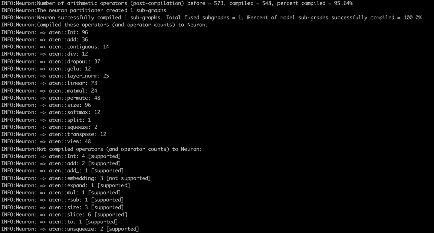
Before we can deploy the Stable Diffusion 2.1 model on AWS Inferentia2 instances, we need to compile the model components using the Neuron SDK. The Neuron SDK, which includes a deep learning compiler, runtime, and tools, compiles and automatically optimizes deep learning models so they can run efficiently on Inf2 instances and extract full performance of the AWS Inferentia2 accelerator. We have examples available for Stable Diffusion 2.1 model on the GitHub repo. This notebook presents an end-to-end example of how to compile a Stable Diffusion model, save the compiled Neuron models, and load it into the runtime for inference.

We use StableDiffusionPipeline from the Hugging Face diffusers library to load and compile the model. We then compile all the components of the model for Neuron using torch_neuronx.trace() and save the optimized model as TorchScript. Compilation processes can be quite memory-intensive, requiring a significant amount of RAM. To circumvent this, before tracing each model, we create a deepcopy of the part of the pipeline that’s being traced. Following this, we delete the pipeline object from memory using del pipe. This technique is particularly useful when compiling on instances with low RAM.

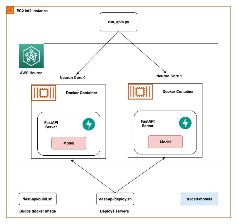
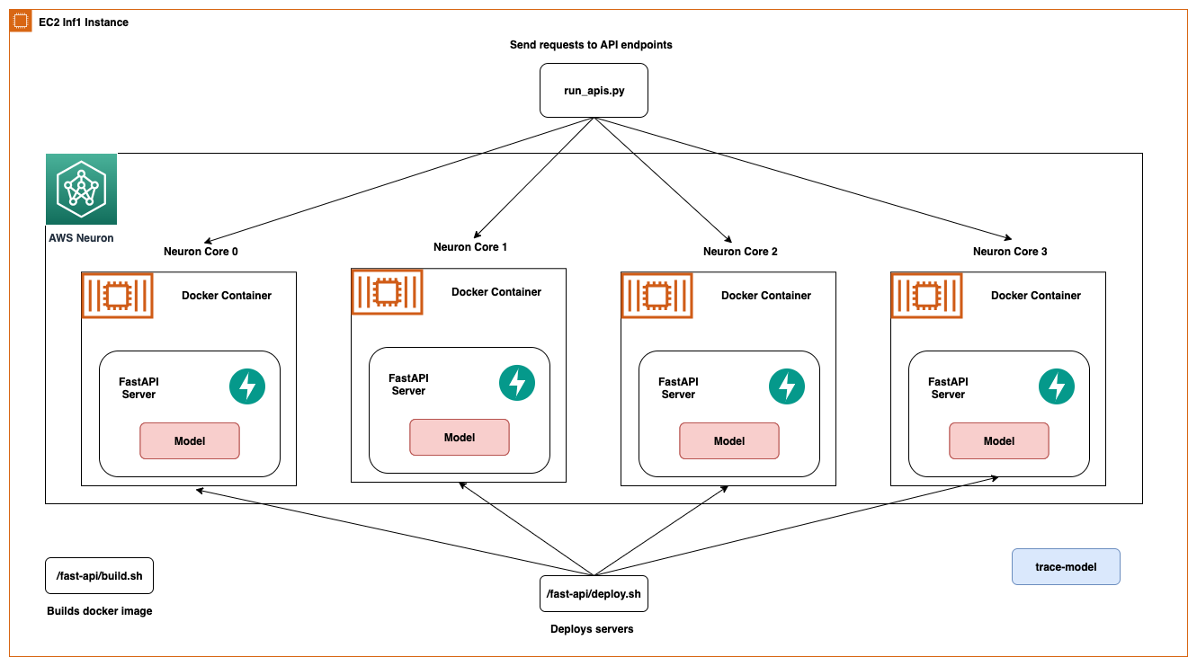
Additionally, we also perform optimizations to the Stable Diffusion models. UNet holds the most computationally intensive aspect of the inference. The UNet component operates on input tensors that have a batch size of two, generating a corresponding output tensor also with a batch size of two, to produce a single image. The elements within these batches are entirely independent of each other. We can take advantage of this behavior to get optimal latency by running one batch on each Neuron core. We compile the UNet for one batch (by using input tensors with one batch), then use the torch_neuronx.DataParallel API to load this single batch model onto each core. The output of this API is a seamless two-batch module: we can pass to the UNet the inputs of two batches, and a two-batch output is returned, but internally, the two single-batch models are running on the two Neuron cores. This strategy optimizes resource utilization and reduces latency.

Compile and deploy a Stable Diffusion model on an Inf2 EC2 instance

To compile and deploy the Stable Diffusion model on an Inf2 EC2 instance, sign to the AWS Management Console and create an inf2.8xlarge instance. Note that an inf2.8xlarge instance is required only for the compilation of the model because compilation requires a higher host memory. The Stable Diffusion model can be hosted on an inf2.xlarge instance. You can find the latest AMI with Neuron libraries using the following AWS Command Line Interface (AWS CLI) command:

aws ec2 describe-images --region us-east-1 --owners amazon 
--filters 'Name=name,Values=Deep Learning AMI Neuron PyTorch 1.13.? (Amazon Linux 2) ????????' 'Name=state,Values=available' 
--query 'reverse(sort_by(Images, &CreationDate))[:1].ImageId' 
--output text

For this example, we created an EC2 instance using the Deep Learning AMI Neuron PyTorch 1.13 (Ubuntu 20.04). You can then create a JupyterLab lab environment by connecting to the instance and running the following steps:

run source /opt/aws_neuron_venv_pytorch/bin/activate
pip install jupyterlab
jupyter-lab

A notebook with all the steps for compiling and hosting the model is located on GitHub.

Let’s look at the compilation steps for one of the text encoder blocks. Other blocks that are part of the Stable Diffusion pipeline can be compiled similarly.

The first step is to load the pre-trained model from Hugging Face. The StableDiffusionPipeline.from_pretrained method loads the pre-trained model into our pipeline object, pipe. We then create a deepcopy of the text encoder from our pipeline, effectively cloning it. The del pipe command is then used to delete the original pipeline object, freeing up the memory that was consumed by it. Here, we are quantizing the model to BF16 weights:

model_id = "stabilityai/stable-diffusion-2-1-base"
pipe = StableDiffusionPipeline.from_pretrained(model_id, torch_dtype=torch.bfloat16)
text_encoder = copy.deepcopy(pipe.text_encoder)
del pipe

This step involves wrapping our text encoder with the NeuronTextEncoder wrapper. The output of a compiled text encoder module will be of dict. We convert it to a list type using this wrapper:

text_encoder = NeuronTextEncoder(text_encoder)

We initialize PyTorch tensor emb with some values. The emb tensor is used as example input for the torch_neuronx.trace function. This function traces our text encoder and compiles it into a format optimized for Neuron. The directory path for the compiled model is constructed by joining COMPILER_WORKDIR_ROOT with the subdirectory text_encoder:

emb = torch.tensor([...])
text_encoder_neuron = torch_neuronx.trace(
        text_encoder.neuron_text_encoder,
        emb,
        compiler_workdir=os.path.join(COMPILER_WORKDIR_ROOT, 'text_encoder'),
        )

The compiled text encoder is saved using torch.jit.save. It’s stored under the file name model.pt in the text_encoder directory of our compiler’s workspace:

text_encoder_filename = os.path.join(COMPILER_WORKDIR_ROOT, 'text_encoder/model.pt')
torch.jit.save(text_encoder_neuron, text_encoder_filename)

The notebook includes similar steps to compile other components of the model: UNet, VAE decoder, and VAE post_quant_conv. After you have compiled all the models, you can load and run the model following these steps:

1. Define the paths for the compiled models.
2. Load a pre-trained StableDiffusionPipeline model, with its configuration specified to use the bfloat16 data type.
3. Load the UNet model onto two Neuron cores using the torch_neuronx.DataParallel API. This allows data parallel inference to be performed, which can significantly speed up model performance.
4. Load the remaining parts of the model (text_encoder, decoder, and post_quant_conv) onto a single Neuron core.

You can then run the pipeline by providing input text as prompts. The following are some pictures generated by the model for the prompts:

• Portrait of renaud sechan, pen and ink, intricate line drawings, by craig mullins, ruan jia, kentaro miura, greg rutkowski, loundraw

• Portrait of old coal miner in 19th century, beautiful painting, with highly detailed face painting by greg rutkowski

• A castle in the middle of a forest

Host Stable Diffusion 2.1 on AWS Inferentia2 and SageMaker

Hosting Stable Diffusion models with SageMaker also requires compilation with the Neuron SDK. You can complete the compilation ahead of time or during runtime using Large Model Inference (LMI) containers. Compilation ahead of time allows for faster model loading times and is the preferred option.

SageMaker LMI containers provide two ways to deploy the model:

• A no-code option where we just provide a serving.properties file with the required configurations
• Bring your own inference script

We look at both solutions and go over the configurations and the inference script (model.py). In this post, we demonstrate the deployment using a pre-compiled model stored in an Amazon Simple Storage Service (Amazon S3) bucket. You can use this pre-compiled model for your deployments.

Configure the model with a provided script

In this section, we show how to configure the LMI container to host the Stable Diffusion models. The SD2.1 notebook available on GitHub. The first step is to create the model configuration package per the following directory structure. Our aim is to use the minimal model configurations needed to host the model. The directory structure needed is as follows:

<config-root-directory> / 
    ├── serving.properties
    │   
    └── model.py [OPTIONAL]

Next, we create the serving.properties file with the following parameters:

%%writefile code_sd/serving.properties
engine=Python
option.entryPoint=djl_python.transformers-neuronx
option.use_stable_diffusion=True
option.model_id=s3url
option.tensor_parallel_degree=2
option.dtype=bf16

The parameters specify the following:

• option.model_id – The LMI containers use s5cmd to load the model from the S3 location and therefore we need to specify the location of where our compiled weights are.
• option.entryPoint – To use the built-in handlers, we specify the transformers-neuronx class. If you have a custom inference script, you need to provide that instead.
• option.dtype – This specifies to load the weights in a specific size. For this post, we use BF16, which further reduces our memory requirements vs. FP32 and lowers our latency due to that.
• option.tensor_parallel_degree – This parameter specifies the number of accelerators we use for this model. The AWS Inferentia2 chip accelerator has two Neuron cores and so specifying a value of 2 means we use one accelerator (two cores). This means we can now create multiple workers to increase the throughput of the endpoint.
• option.engine – This is set to Python to indicate we will not be using other compilers like DeepSpeed or Faster Transformer for this hosting.

Bring your own script

If you want to bring your own custom inference script, you need to remove the option.entryPoint from serving.properties. The LMI container in that case will look for a model.py file in the same location as the serving.properties and use that to run the inferencing.

Create your own inference script (model.py)

Creating your own inference script is relatively straightforward using the LMI container. The container requires your model.py file to have an implementation of the following method:

def handle(inputs: Input) which returns an object of type Outputs

Let’s examine some of the critical areas of the attached notebook, which demonstrates the bring your own script function.

Replace the cross_attention module with the optimized version:

# Replace original cross-attention module with custom cross-attention module for better performance
    CrossAttention.get_attention_scores = get_attention_scores
Load the compiled weights for the following
text_encoder_filename = os.path.join(COMPILER_WORKDIR_ROOT, 'text_encoder.pt')
decoder_filename = os.path.join(COMPILER_WORKDIR_ROOT, 'vae_decoder.pt')
unet_filename = os.path.join(COMPILER_WORKDIR_ROOT, 'unet.pt')
post_quant_conv_filename =. os.path.join(COMPILER_WORKDIR_ROOT, 'vae_post_quant_conv.pt')

These are the names of the compiled weights file we used when creating the compilations. Feel free to change the file names, but make sure your weights file names match what you specify here.

Then we need to load them using the Neuron SDK and set these in the actual model weights. When loading the UNet optimized weights, note we are also specifying the number of Neuron cores we need to load these onto. Here, we load to a single accelerator with two cores:

# Load the compiled UNet onto two neuron cores.
    pipe.unet = NeuronUNet(UNetWrap(pipe.unet))
    logging.info(f"Loading model: unet:created")
    device_ids = [idx for idx in range(tensor_parallel_degree)]
   
    pipe.unet.unetwrap = torch_neuronx.DataParallel(torch.jit.load(unet_filename), device_ids, set_dynamic_batching=False)
   
 
    # Load other compiled models onto a single neuron core.
 
    # - load encoders
    pipe.text_encoder = NeuronTextEncoder(pipe.text_encoder)
    clip_compiled = torch.jit.load(text_encoder_filename)
    pipe.text_encoder.neuron_text_encoder = clip_compiled
    #- load decoders
    pipe.vae.decoder = torch.jit.load(decoder_filename)
    pipe.vae.post_quant_conv = torch.jit.load(post_quant_conv_filename)

Running the inference with a prompt invokes the pipe object to generate an image.

Create the SageMaker endpoint

We use Boto3 APIs to create a SageMaker endpoint. Complete the following steps:

1. Create the tarball with just the serving and the optional model.py files and upload it to Amazon S3.
2. Create the model using the image container and the model tarball uploaded earlier.
3. Create the endpoint config using the following key parameters:
   1. Use an ml.inf2.xlarge instance.
   2. Set ContainerStartupHealthCheckTimeoutInSeconds to 240 to ensure the health check starts after the model is deployed.
   3. Set VolumeInGB to a larger value so it can be used for loading the model weights that are 32 GB in size.

Create a SageMaker model

After you create the model.tar.gz file and upload it to Amazon S3, we need to create a SageMaker model. We use the LMI container and the model artifact from the previous step to create the SageMaker model. SageMaker allows us to customize and inject various environment variables. For this workflow, we can leave everything as default. See the following code:

inference_image_uri = (
    f"763104351884.dkr.ecr.{region}.amazonaws.com/djl-inference:0 djl-serving-inf2"
)

Create the model object, which essentially creates a lockdown container that is loaded onto the instance and used for inferencing:

model_name = name_from_base(f"inf2-sd")
create_model_response = boto3_sm_client.create_model(
    ModelName=model_name,
    ExecutionRoleArn=role,
    PrimaryContainer={"Image": inference_image_uri, "ModelDataUrl": s3_code_artifact},
)

Create a SageMaker endpoint

In this demo, we use an ml.inf2.xlarge instance. We need to set the VolumeSizeInGB parameters to provide the necessary disk space to load the model and the weights. This parameter is applicable to instances supporting the Amazon Elastic Block Store (Amazon EBS) volume attachment. We can leave the model download timeout and container startup health check to a higher value, which will give adequate time for the container to pull the weights from Amazon S3 and load into the AWS Inferentia2 accelerators. For more details, refer to CreateEndpointConfig.

endpoint_config_response = boto3_sm_client.create_endpoint_config(

EndpointConfigName=endpoint_config_name,
    ProductionVariants=[
        {
            "VariantName": "variant1",
            "ModelName": model_name,
            "InstanceType": "ml.inf2.xlarge", # - 
            "InitialInstanceCount": 1,
            "ContainerStartupHealthCheckTimeoutInSeconds": 360, 
            "VolumeSizeInGB": 400
        },
    ],
)

Lastly, we create a SageMaker endpoint:

create_endpoint_response = boto3_sm_client.create_endpoint(
    EndpointName=f"{endpoint_name}", EndpointConfigName=endpoint_config_name
)

Invoke the model endpoint

This is a generative model, so we pass in the prompt that the model uses to generate the image. The payload is of the type JSON:

response_model = boto3_sm_run_client.invoke_endpoint(

EndpointName=endpoint_name,
    Body=json.dumps(
        {
            "prompt": "Mountain Landscape", 
            "parameters": {} # 
        }
    ), 
    ContentType="application/json",
)

Benchmarking the Stable Diffusion model on Inf2

We ran a few tests to benchmark the Stable Diffusion model with BF 16 data type on Inf2, and we are able to derive latency numbers that rival or exceed some of the other accelerators for Stable Diffusion. This, coupled with the lower cost of AWS Inferentia2 chips, makes this an extremely valuable proposition.

The following numbers are from the Stable Diffusion model deployed on an inf2.xl instance. For more information about costs, refer to Amazon EC2 Inf2 Instances.

Conclusion

In this post, we dove deep into the compilation, optimization, and deployment of the Stable Diffusion 2.1 model using Inf2 instances. We also demonstrated deployment of Stable Diffusion models using SageMaker. Inf2 instances also deliver great price performance for Stable Diffusion 1.5. To learn more about why Inf2 instances are great for generative AI and large language models, refer to Amazon EC2 Inf2 Instances for Low-Cost, High-Performance Generative AI Inference are Now Generally Available. For performance details, refer to Inf2 Performance. Check out additional examples on the GitHub repo.

Special thanks to Matthew Mcclain, Beni Hegedus, Kamran Khan, Shruti Koparkar, and Qing Lan for reviewing and providing valuable inputs.

About the Authors

Vivek Gangasani is a Senior Machine Learning Solutions Architect at Amazon Web Services. He works with machine learning startups to build and deploy AI/ML applications on AWS. He is currently focused on delivering solutions for MLOps, ML inference, and low-code ML. He has worked on projects in different domains, including natural language processing and computer vision.

K.C. Tung is a Senior Solution Architect in AWS Annapurna Labs. He specializes in large deep learning model training and deployment at scale in cloud. He has a Ph.D. in molecular biophysics from the University of Texas Southwestern Medical Center in Dallas. He has spoken at AWS Summits and AWS Reinvent. Today he helps customers to train and deploy large PyTorch and TensorFlow models in AWS cloud. He is the author of two books: Learn TensorFlow Enterprise and TensorFlow 2 Pocket Reference.

Rupinder Grewal is a Sr Ai/ML Specialist Solutions Architect with AWS. He currently focuses on serving of models and MLOps on SageMaker. Prior to this role he has worked as Machine Learning Engineer building and hosting models. Outside of work he enjoys playing tennis and biking on mountain trails.

Read More

Breakthroughs in artificial intelligence (AI) and machine learning (ML) have been in the headlines for months—and for good reason. The emerging and evolving capabilities of this technology promises new business opportunities for customer across all sectors and industries. But the speed of this revolution has made it harder for organizations and consumers to assess what these breakthroughs mean for them specifically.

Over the years, AWS has invested in the democratizing of access to—and understanding of —AI, ML and generative AI. Through announcements around the latest developments in generative AI and the establishment of a $100 million Generative AI Innovation Center program, Amazon Web Services (AWS) has been at the forefront of helping drive understanding about the role that these innovations can play in the lives of both individuals and organizations. To help you understand your options in relation to AI and ML, AWS has published two new guides: the AWS Cloud Adoption Framework for Artificial Intelligence, Machine Learning, and Generative AI and the Getting Started Resource Center machine learning decision guide.

AWS CAF for AI, ML, and Generative AI

The AWS Cloud Adoption Framework for Artificial Intelligence, Machine Learning, and Generative AI (CAF-AI) is designed to help you navigate your AI journey. It’s a mental model for organizations that strive to generate business value from AI/ML. Based on our own—and our customers’—experience, we provide in this framework of best practices for an AI transformation and accelerate business outcomes through innovative use of AI on AWS.

Used by customers and partner teams, CAF-AI helps derive, prioritize, evolve, and communicate a strategy for AI transformation. The following figure shows how we simplify an AI journey through CAF-AI: by working backward from business outcomes (1) to the opportunities that AI, ML, and generative AI provide (2), across your transformation domains (3) and your foundational capabilities (4) through an iterative process (5) of assessing, deriving, and implementing action items for an AI strategy.

In CAF-AI, we describe the AI/ML journey you may experience as your organizational capabilities on AI and ML mature. To guide you, we zoom in on the evolution of foundational capabilities that we have observed assist an organization to grow its maturity in AI further.

We also provide prescriptive guidance through an overview of the target state of these foundational capabilities and explain how to evolve them step by step to generate business value along the way. The following figure shows these foundational capabilities for cloud and AI/ML adoption. A capability is an organizational ability to use processes to deploy resources (such as people, technology, and other tangible or intangible assets) to achieve an outcome. Because the CAF-AI is a living index of knowledge, you can expect it to grow and change over time.

Designed as a starting and orientation point throughout a customer’s ML and AI journey, CAF-AI is intended to be a document that organizations can draw inspiration from as they shape their mid-term AI and ML agenda and try to understand the important topics and perspectives that influence it. Depending on where you are at on your AI/ML journey, you might focus on a specific section and hone your skills there, or use the whole document to judge maturity and help direct near-term improvement areas.

Because the business problem space to which AI/ML can be applied isn’t a single function or domain, it applies across all functions of businesses and all industry domains where you are looking for ways to reset the playing field in markets where AI/ML does make an economical difference. The AWS Cloud Adoption Framework for Artificial Intelligence, Machine Learning, and Generative AI is one of the many tools AWS provides to help you achieve this outcome. As AI/ML enables solutions and solution paths to problems that have remained uneconomical to solve for decades (or were technically impossible to tackle without AI/ML), the resulting business outcomes can be profound.

The Getting Started Resource Center machine learning decision guide

AWS has always been about choice. As you ramp up your use of AI, it is paramount that you have the right support in choosing the best service, model, and infrastructure for your business needs. The Getting Started Resource Center machine learning decision guide is designed to provide you with a detailed overview of the AI and ML services offered by AWS, and provide structured guidance on how to choose the services that might be right for you and your use cases.

The decision guide can also help you articulate and consider the criteria that will inform your choices. For example, it describes the range of AWS ML services (see the following screenshot), each of which caters to different levels of management requirement, depending on how much control and customization you need.

The guide also explains the unique capabilities of AWS services in realizing the power of foundation models and where you can make the most of this fast-evolving branch of machine learning.

It offers details on specific services, links to detailed, service-level technical guides, a comparison table that highlights the unique capabilities of key services, and criteria for selecting AI and ML services. It also provides a curated set of links to key resources that can help you get started in using AI, ML, and generative AI services on AWS.

If you want to understand the breadth of AI, ML, and generative AI offerings provided by AWS, this decision guide is a great place to start.

Conclusion

The Getting Started Resource Center machine learning decision guide, together with the AWS Cloud Adoption Framework for Artificial Intelligence, Machine Learning, and Generative AI, covers the technical and non-technical questions that we often hear. We hope you find these new resources useful and look forward to your feedback on them.

About the Authors

Caleb Wilkinson has more than a decade of experience building AI solutions. As a Senior Machine Learning Strategist at AWS, Caleb pioneers innovative applications of AI that push the boundaries of possibility and helps organizations benefit responsibly from artificial intelligence. He is the co-author of CAF-AI.

Alexander Wöhlke has a decade of experience in AI and ML. He is Senior Machine Learning Strategist and Technical Product Manager at the AWS Generative AI Innovation Center. He works with large organizations on their AI-Strategy and helps them take calculated risks at the forefront of technological development. He is the co-author of CAF-AI.

Geof Wheelwright manages the AWS decision content team, which writes and develops the growing collection of decision guides on the AWS Getting Started Resource Center. His team created the Choosing an AWS machine learning decision guide. He has enjoyed working with AI and its ancestors since first being introduced to simple, text-based Apple II versions of ELIZA in the early 1980s.

Read More

Generative AI Foundations on AWS is a new technical deep dive course that gives you the conceptual fundamentals, practical advice, and hands-on guidance to pre-train, fine-tune, and deploy state-of-the-art foundation models on AWS and beyond. Developed by AWS generative AI worldwide foundations lead Emily Webber, this free hands-on course and the supporting GitHub source code launched via AWS Youtube. If you are looking for a curated playlist of the top resources, concepts, and guidance to get up to speed on foundation models, and especially those that unlock generative capabilities in your data science and machine learning projects, then look no further.

During this 8-hour deep dive, you will be introduced to the key techniques, services, and trends that will help you understand foundation models from the ground up. This means breaking down theory, mathematics, and abstract concepts combined with hands-on exercises to gain functional intuition for practical application. Throughout the course, we focus on a wide spectrum of progressively complex generative AI techniques, giving you a strong base to understand, design, and apply your own models for the best performance. We’ll start with recapping foundation models, understanding where they come from, how they work, how they relate to generative AI, and what you can to do customize them. You’ll then learn about picking the right foundation model to suit your use case.

Once you’ve developed a strong contextual understanding of foundation models and how to use them, you’ll be introduced to the core subject of this course: pre-training new foundation models. You’ll learn why you’d want to do this as well as how and where it’s competitive. You’ll even learn how to use the scaling laws to pick the right model, dataset, and compute sizes. We’ll cover preparing training datasets at scale on AWS, including picking the right instances and storage techniques. We’ll cover fine-tuning your foundation models, evaluating recent techniques, and understanding how to run these with your scripts and models. We’ll dive into reinforcement learning with human feedback, exploring how to use it skillfully and at scale to truly maximize your foundation model performance.

Finally, you’ll learn how to apply theory to production by deploying your new foundation model on Amazon SageMaker, including across multiple GPUs and using top design patterns like retrieval augmented generation and chained dialogue. As an added bonus, we’ll walk you through a Stable Diffusion deep dive, prompt engineering best practices, standing up LangChain, and more.

More of a reader than a video consumer? You can check out my 15-chapter book “Pretrain Vision and Large Language Models in Python: End-to-end techniques for building and deploying foundation models on AWS,” which released May 31, 2023, with Packt publishing and is available now on Amazon. Want to jump right into the code? I’m with you—every video starts with a 45-minute overview of the key concepts and visuals. Then I’ll give you a 15-minute walkthrough of the hands-on portion. All of the example notebooks and supporting code will ship in a public repository, which you can use to step through on your own. Feel free to reach out to me on Medium, LinkedIn, GitHub, or through your AWS teams. Learn more about generative AI on AWS.

Happy trails!

Course outline

1. Introduction to Foundation Models

2. Picking the right foundation model

3. Using pretrained foundation models: prompt engineering and fine-tuning

4. Pretraining a new foundation model

5. Preparing data and training at scale

6. Reinforcement learning with human feedback

7. Deploying a foundation model

About the author

Emily Webber joined AWS just after SageMaker launched, and has been trying to tell the world about it ever since! Outside of building new ML experiences for customers, Emily enjoys meditating and studying Tibetan Buddhism.

Read More

As a pioneer in artificial intelligence and machine learning, AWS is committed to developing and deploying generative AI responsibly

As one of the most transformational innovations of our time, generative AI continues to capture the world’s imagination, and we remain as committed as ever to harnessing it responsibly. With a team of dedicated responsible AI experts, complemented by our engineering and development organization, we continually test and assess our products and services to define, measure, and mitigate concerns about accuracy, fairness, intellectual property, appropriate use, toxicity, and privacy. And while we don’t have all of the answers today, we are working alongside others to develop new approaches and solutions to address these emerging challenges. We believe we can both drive innovation in AI, while continuing to implement the necessary safeguards to protect our customers and consumers.

At AWS, we know that generative AI technology and how it is used will continue to evolve, posing new challenges that will require additional attention and mitigation. That’s why Amazon is actively engaged with organizations and standard bodies focused on the responsible development of next-generation AI systems including NIST, ISO, the Responsible AI Institute, and the Partnership on AI. In fact, last week at the White House, Amazon signed voluntary commitments to foster the safe, responsible, and effective development of AI technology. We are eager to share knowledge with policymakers, academics, and civil society, as we recognize the unique challenges posed by generative AI will require ongoing collaboration.

This commitment is consistent with our approach to developing our own generative AI services, including building foundation models (FMs) with responsible AI in mind at each stage of our comprehensive development process. Throughout design, development, deployment, and operations we consider a range of factors including 1/ accuracy, e.g., how closely a summary matches the underlying document; whether a biography is factually correct; 2/ fairness, e.g., whether outputs treat demographic groups similarly; 3/ intellectual property and copyright considerations; 4/ appropriate usage, e.g., filtering out user requests for legal advice, medical diagnoses, or illegal activities, 5/ toxicity, e.g., hate speech, profanity, and insults; and 6/ privacy, e.g., protecting personal information and customer prompts. We build solutions to address these issues into our processes for acquiring training data, into the FMs themselves, and into the technology that we use to pre-process user prompts and post-process outputs. For all our FMs, we invest actively to improve our features, and to learn from customers as they experiment with new use cases.

For example, Amazon’s Titan FMs are built to detect and remove harmful content in the data that customers provide for customization, reject inappropriate content in the user input, and filter the model’s outputs containing inappropriate content (such as hate speech, profanity, and violence).

To help developers build applications responsibly, Amazon CodeWhisperer provides a reference tracker that displays the licensing information for a code recommendation and provides link to the corresponding open-source repository when necessary. This makes it easier for developers to decide whether to use the code in their project and make the relevant source code attributions as they see fit. In addition, Amazon CodeWhisperer filters out code recommendations that include toxic phrases, and recommendations that indicate bias.

Through innovative services like these, we will continue to help our customers realize the benefits of generative AI, while collaborating across the public and private sectors to ensure we’re doing so responsibly. Together, we will build trust among customers and the broader public, as we harness this transformative new technology as a force for good.

About the Author

Peter Hallinan leads initiatives in the science and practice of Responsible AI at AWS AI, alongside a team of responsible AI experts. He has deep expertise in AI (PhD, Harvard) and entrepreneurship (Blindsight, sold to Amazon). His volunteer activities have included serving as a consulting professor at the Stanford University School of Medicine, and as the president of the American Chamber of Commerce in Madagascar. When possible, he’s off in the mountains with his children: skiing, climbing, hiking and rafting

Read More

With recent advancements in generative AI, there are lot of discussions happening on how to use generative AI across different industries to solve specific business problems. Generative AI is a type of AI that can create new content and ideas, including conversations, stories, images, videos, and music. It is all backed by very large models that are pre-trained on vast amounts of data and commonly referred to as foundation models (FMs). These FMs can perform a wide range of tasks that span multiple domains, like writing blog posts, generating images, solving math problems, engaging in dialog, and answering questions based on a document. The size and general-purpose nature of FMs make them different from traditional ML models, which typically perform specific tasks, like analyzing text for sentiment, classifying images, and forecasting trends.

While organizations are looking to use the power of these FMs, they also want the FM-based solutions to be running in their own protected environments. Organizations operating in heavily regulated spaces like global financial services and healthcare and life sciences have auditory and compliance requirements to run their environment in their VPCs. In fact, a lot of times, even direct internet access is disabled in these environments to avoid exposure to any unintended traffic, both ingress and egress.

Amazon SageMaker JumpStart is an ML hub offering algorithms, models, and ML solutions. With SageMaker JumpStart, ML practitioners can choose from a growing list of best performing open source FMs. It also provides the ability to deploy these models in your own Virtual Private Cloud (VPC).

In this post, we demonstrate how to use JumpStart to deploy a Flan-T5 XXL model in a VPC with no internet connectivity. We discuss the following topics:

• How to deploy a foundation model using SageMaker JumpStart in a VPC with no internet access
• Advantages of deploying FMs via SageMaker JumpStart models in VPC mode
• Alternate ways to customize deployment of foundation models via JumpStart

Apart from FLAN-T5 XXL, JumpStart provides lot of different foundation models for various tasks. For the complete list, check out Getting started with Amazon SageMaker JumpStart.

Solution overview

As part of the solution, we cover the following steps:

1. Set up a VPC with no internet connection.
2. Set up Amazon SageMaker Studio using the VPC we created.
3. Deploy the generative AI Flan T5-XXL foundation model using JumpStart in the VPC with no internet access.

The following is an architecture diagram of the solution.

Let’s walk through the different steps to implement this solution.

Prerequisites

To follow along with this post, you need the following:

• Access to an AWS account. For details, check out Creating an AWS account.
• An AWS Identity and Access Management (IAM) role with permissions to deploy the AWS CloudFormation templates used in this solution and manage resources as part of the solution.

Set up a VPC with no internet connection

Create a new CloudFormation stack by using the 01_networking.yaml template. This template creates a new VPC and adds two private subnets across two Availability Zones with no internet connectivity. It then deploys gateway VPC endpoints for accessing Amazon Simple Storage Service (Amazon S3) and interface VPC endpoints for SageMaker and a few other services to allow the resources in the VPC to connect to AWS services via AWS PrivateLink.

Provide a stack name, such as No-Internet, and complete the stack creation process.

This solution is not highly available because the CloudFormation template creates interface VPC endpoints only in one subnet to reduce costs when following the steps in this post.

Set up Studio using the VPC

Create another CloudFormation stack using 02_sagemaker_studio.yaml, which creates a Studio domain, Studio user profile, and supporting resources like IAM roles. Choose a name for the stack; for this post, we use the name SageMaker-Studio-VPC-No-Internet. Provide the name of the VPC stack you created earlier (No-Internet) as the CoreNetworkingStackName parameter and leave everything else as default.

Wait until AWS CloudFormation reports that the stack creation is complete. You can confirm the Studio domain is available to use on the SageMaker console.

To verify the Studio domain user has no internet access, launch Studio using the SageMaker console. Choose File, New, and Terminal, then attempt to access an internet resource. As shown in the following screenshot, the terminal will keep waiting for the resource and eventually time out.

This proves that Studio is operating in a VPC that doesn’t have internet access.

Deploy the generative AI foundation model Flan T5-XXL using JumpStart

We can deploy this model via Studio as well as via API. JumpStart provides all the code to deploy the model via a SageMaker notebook accessible from within Studio. For this post, we showcase this capability from the Studio.

• On the Studio welcome page, choose JumpStart under Prebuilt and automated solutions.

• Choose the Flan-T5 XXL model under Foundation Models.

• By default, it opens the Deploy tab. Expand the Deployment Configuration section to change the hosting instance and endpoint name, or add any additional tags. There is also an option to change the S3 bucket location where the model artifact will be stored for creating the endpoint. For this post, we leave everything at its default values. Make a note of the endpoint name to use while invoking the endpoint for making predictions.

• Expand the Security Settings section, where you can specify the IAM role for creating the endpoint. You can also specify the VPC configurations by providing the subnets and security groups. The subnet IDs and security group IDs can be found from the VPC stack’s Outputs tab on the AWS CloudFormation console. SageMaker JumpStart requires at least two subnets as part of this configuration. The subnets and security groups control access to and from the model container.

NOTE: Irrespective of whether the SageMaker JumpStart model is deployed in the VPC or not, the model always runs in network isolation mode, which isolates the model container so no inbound or outbound network calls can be made to or from the model container. Because we’re using a VPC, SageMaker downloads the model artifact through our specified VPC. Running the model container in network isolation doesn’t prevent your SageMaker endpoint from responding to inference requests. A server process runs alongside the model container and forwards it the inference requests, but the model container doesn’t have network access.

• Choose Deploy to deploy the model. We can see the near-real-time status of the endpoint creation in progress. The endpoint creation may take 5–10 minutes to complete.

Observe the value of the field Model data location on this page. All the SageMaker JumpStart models are hosted on a SageMaker managed S3 bucket (s3://jumpstart-cache-prod-{region}). Therefore, irrespective of which model is picked from JumpStart, the model gets deployed from the publicly accessible SageMaker JumpStart S3 bucket and the traffic never goes to the public model zoo APIs to download the model. This is why the model endpoint creation started successfully even when we’re creating the endpoint in a VPC that doesn’t have direct internet access.

The model artifact can also be copied to any private model zoo or your own S3 bucket to control and secure model source location further. You can use the following command to download the model locally using the AWS Command Line Interface (AWS CLI):

aws s3 cp s3://jumpstart-cache-prod-eu-west-1/huggingface-infer/prepack/v1.0.2/infer-prepack-huggingface-text2text-flan-t5-xxl.tar.gz .

• After a few minutes, the endpoint gets created successfully and shows the status as In Service. Choose Open Notebook in the Use Endpoint from Studio section. This is a sample notebook provided as part of the JumpStart experience to quickly test the endpoint.

• In the notebook, choose the image as Data Science 3.0 and the kernel as Python 3. When the kernel is ready, you can run the notebook cells to make predictions on the endpoint. Note that the notebook uses the invoke_endpoint() API from the AWS SDK for Python to make predictions. Alternatively, you can use the SageMaker Python SDK’s predict() method to achieve the same result.

This concludes the steps to deploy the Flan-T5 XXL model using JumpStart within a VPC with no internet access.

Advantages of deploying SageMaker JumpStart models in VPC mode

The following are some of the advantages of deploying SageMaker JumpStart models in VPC mode:

• Because SageMaker JumpStart doesn’t download the models from a public model zoo, it can be used in fully locked-down environments as well where there is no internet access
• Because the network access can be limited and scoped down for SageMaker JumpStart models, this helps teams improve the security posture of the environment
• Due to the VPC boundaries, access to the endpoint can also be limited via subnets and security groups, which adds an extra layer of security

Alternate ways to customize deployment of foundation models via SageMaker JumpStart

In this section, we share some alternate ways to deploy the model.

Use SageMaker JumpStart APIs from your preferred IDE

Models provided by SageMaker JumpStart don’t require you to access Studio. You can deploy them to SageMaker endpoints from any IDE, thanks to the JumpStart APIs. You could skip the Studio setup step discussed earlier in this post and use the JumpStart APIs to deploy the model. These APIs provide arguments where VPC configurations can be supplied as well. The APIs are part of the SageMaker Python SDK itself. For more information, refer to Pre-trained models.

Use notebooks provided by SageMaker JumpStart from SageMaker Studio

SageMaker JumpStart also provides notebooks to deploy the model directly. On the model detail page, choose Open notebook to open a sample notebook containing the code to deploy the endpoint. The notebook uses SageMaker JumpStart Industry APIs that allow you to list and filter the models, retrieve the artifacts, and deploy and query the endpoints. You can also edit the notebook code per your use case-specific requirements.

Clean up resources

Check out the CLEANUP.md file to find detailed steps to delete the Studio, VPC, and other resources created as part of this post.

Troubleshooting

If you encounter any issues in creating the CloudFormation stacks, refer to Troubleshooting CloudFormation.

Conclusion

Generative AI powered by large language models is changing how people acquire and apply insights from information. However, organizations operating in heavily regulated spaces are required to use the generative AI capabilities in a way that allows them to innovate faster but also simplifies the access patterns to such capabilities.

We encourage you to try out the approach provided in this post to embed generative AI capabilities in your existing environment while still keeping it inside your own VPC with no internet access. For further reading on SageMaker JumpStart foundation models, check out the following:

• Domain-adaptation Fine-tuning of Foundation Models in Amazon SageMaker JumpStart on Financial data
• Implementing MLOps practices with Amazon SageMaker JumpStart pre-trained models

About the authors

Vikesh Pandey is a Machine Learning Specialist Solutions Architect at AWS, helping customers from financial industries design and build solutions on generative AI and ML. Outside of work, Vikesh enjoys trying out different cuisines and playing outdoor sports.

Mehran Nikoo is a Senior Solutions Architect at AWS, working with Digital Native businesses in the UK and helping them achieve their goals. Passionate about applying his software engineering experience to machine learning, he specializes in end-to-end machine learning and MLOps practices.

Read More

This blog post was co-authored, and includes an introduction, by Zilong Bai, senior natural language processing engineer at Patsnap.

You’re likely familiar with the autocomplete suggestion feature when you search for something on Google or Amazon. Although the search terms in these scenarios are pretty common keywords or expressions that we use in daily life, in some cases search terms are very specific to the scenario. Patent search is one of them. Recently, the AWS Generative AI Innovation Center collaborated with Patsnap to implement a feature to automatically suggest search keywords as an innovation exploration to improve user experiences on their platform.

Patsnap provides a global one-stop platform for patent search, analysis, and management. They use big data (such as a history of past search queries) to provide many powerful yet easy-to-use patent tools. These tools have enabled Patsnap’s global customers to have a better understanding of patents, track recent technological advances, identify innovation trends, and analyze competitors in real time.

At the same time, Patsnap is embracing the power of machine learning (ML) to develop features that can continuously improve user experiences on the platform. A recent initiative is to simplify the difficulty of constructing search expressions by autofilling patent search queries using state-of-the-art text generation models. Patsnap had trained a customized GPT-2 model for such a purpose. Because there is no such existing feature in a patent search engine (to their best knowledge), Patsnap believes adding this feature will increase end-user stickiness.

However, in their recent experiments, the inference latency and queries per second (QPS) of a PyTorch-based GPT-2 model couldn’t meet certain thresholds that can justify its business value. To tackle this challenge, AWS Generative AI Innovation Center scientists explored a variety of solutions to optimize GPT-2 inference performance, resulting in lowering the model latency by 50% on average and improving the QPS by 200%.

Large language model inference challenges and optimization approaches

In general, applying such a large model in a real-world production environment is non-trivial. The prohibitive computation cost and latency of PyTorch-based GPT-2 made it difficult to be widely adopted from a business operation perspective. In this project, our objective is to significantly improve the latency with reasonable computation costs. Specifically, Patsnap requires the following:

• The average latency of model inference for generating search expressions needs to be controlled within 600 milliseconds in real-time search scenarios
• The model requires high throughput and QPS to do a large number of searches per second during peak business hours

In this post, we discuss our findings using Amazon Elastic Compute Cloud (Amazon EC2) instances, featuring GPU-based instances using NVIDIA TensorRT.

In a short summary, we use NVIDIA TensorRT to optimize the latency of GPT-2 and deploy it to an Amazon SageMaker endpoint for model serving, which reduces the average latency from 1,172 milliseconds to 531 milliseconds

In the following sections, we go over the technical details of the proposed solutions with key code snippets and show comparisons with the customer’s status quo based on key metrics.

GPT-2 model overview

Open AI’s GPT-2 is a large transformer-based language model with 1.5 billion parameters, trained on the WebText dataset, containing 8 million web pages. The GPT-2 is trained with a simple objective: predict the next word, given all of the previous words within some text. The diversity of the dataset causes this simple goal to contain naturally occurring demonstrations of many tasks across diverse domains. GPT-2 displays a broad set of capabilities, including the ability to generate conditional synthetic text samples of unprecedented quality, where we prime the model with an input and let it generate a lengthy continuation. In this situation, we exploit it to generate search queries. As GPT models keep growing larger, inference costs are continuously rising, which increases the need to deploy these models with acceptable cost.

Achieve low latency on GPU instances via TensorRT

TensorRT is a C++ library for high-performance inference on NVIDIA GPUs and deep learning accelerators, supporting major deep learning frameworks such as PyTorch and TensorFlow. Previous studies have shown great performance improvement in terms of model latency. Therefore, it’s an ideal choice for us to reduce the latency of the target model on NVIDIA GPUs.

We are able to achieve a significant reduction in GPT-2 model inference latency with a TensorRT-based model on NVIDIA GPUs. The TensorRT-based model is deployed via SageMaker for performance tests. In this post, we show the steps to convert the original PyTorch-based GPT-2 model to a TensorRT-based model.

Converting the PyTorch-based GPT-2 to the TensorRT-based model is not difficult via the official tool provided by NVIDIA. In addition, with such straightforward conversions, no obvious model accuracy degradation has been observed. In general, there are three steps to follow:

1. Analyze your GPT-2. As of this writing, NVIDIA’s conversion tool only supports Hugging Face’s version of GPT-2 model. If the current GPT-2 model isn’t the original version, you need to modify it accordingly. It’s recommended to strip out custom code from the original GPT-2 implementation of Hugging Face, which is very helpful for the conversion.
2. Install the required Python packages. The conversion process first converts the PyTorch-based model to the ONNX model and then converts the ONNX-based model to the TensorRT-based model. The following Python packages are needed for this two-step conversion:

tabulate
toml
torch
sentencepiece==0.1.95
onnx==1.9.0
onnx_graphsurgeon
polygraphy
transformers

3. Convert your model. The following code contains the functions for the two-step conversion:

def torch2onnx():
    metadata = NetworkMetadata(variant=GPT2_VARIANT, precision=Precision(fp16=True), other=GPT2Metadata(kv_cache=False))
    gpt2 = GPT2TorchFile(model.to('cpu'), metadata)
    onnx_path = ('Your own path to save ONNX-based model') # e.g, ./model_fp16.onnx
    gpt2.as_onnx_model(onnx_path, force_overwrite=False)
    return onnx_path, metadata
   
def onnx2trt(onnx_path, metadata):
    trt_path = 'Your own path to save TensorRT-based model' # e.g., ./model_fp16.onnx.engine
    batch_size = 10
    max_sequence_length = 42
    profiles = [Profile().add(
        "input_ids",
        min=(1, 1),
        opt=(batch_size, max_sequence_length // 2),
        max=(batch_size, max_sequence_length),
    )]
    gpt2_engine = GPT2ONNXFile(onnx_path, metadata).as_trt_engine(output_fpath=trt_path, profiles=profiles)
    gpt2_trt = GPT2TRTDecoder(gpt2_engine, metadata, config, max_sequence_length=42, batch_size=10)

Latency comparison: PyTorch vs. TensorRT

JMeter is used for performance benchmarking in this project. JMeter is an Apache project that can be used as a load testing tool for analyzing and measuring the performance of a variety of services. We record the QPS and latency of the original PyTorch-based model and our converted TensorRT-based GPT-2 model on an AWS P3.2xlarge instance. As we show later in this post, due to the powerful acceleration ability of TensorRT, the latency of GPT-2 is significantly reduced. When the request concurrency is 1, the average latency has been reduced by 274 milliseconds (2.9 times faster). From the perspective of QPS, it is increased to 7 from 2.4, which is around a 2.9 times boost compared to the original PyTorch-based model. Moreover, as the concurrency increases, QPS keeps increasing. This suggests lower costs with acceptable latency increase (but still much faster than the original model).

The following table compares latency:

Deploy TensorRT-based GPT-2 with SageMaker and a custom container

TensorRT-based GPT-2 requires a relatively recent TensorRT version, so we choose the bring your own container (BYOC) mode of SageMaker to deploy our model. BYOC mode provides a flexible way to deploy the model, and you can build customized environments in your own Docker container. In this section, we show how to build your own container, deploy your own GPT-2 model, and test with the SageMaker endpoint API.

Build your own container

The container’s file directory is presented in the following code. Specifically, Dockerfile and build.sh are used to build the Docker container. gpt2 and predictor.py implement the model and the inference API. serve, nginx.conf, and wsgi.py provide the configuration for the NGINX web server.

container
├── Dockerfile    # build our docker based on this file.
├── build.sh      # create our own image and push it to Amazon ECR
├── gpt2          # model directory
├── predictor.py  # backend function for invoke the model
├── serve         # web server setting file
├── nginx.conf    # web server setting file
└── wsgi.py       # web server setting file

You can run sh ./build.sh to build the container.

Deploy to a SageMaker endpoint

After you have built a container to run the TensorRT-based GPT-2, you can enable real-time inference via a SageMaker endpoint. Use the following code snippets to create the endpoint and deploy the model to the endpoint using the corresponding SageMaker APIs:

import boto3from time import gmtime, strftime
from sagemaker import get_execution_role

sm_client = boto3.client(service_name='sagemaker')
runtime_sm_client = boto3.client(service_name='sagemaker-runtime')
account_id = boto3.client('sts').get_caller_identity()['Account']
region = boto3.Session().region_name
s3_bucket = '${Your s3 bucket}'
role = get_execution_role()
model_name = '${Your Model Name}'
# you need to upload your container to S3 first
container = '${Your Image Path}'
instance_type = 'ml.p3.2xlarge'
container = {
    'Image': container
}
create_model_response = sm_client.create_model(
    ModelName = model_name,
    ExecutionRoleArn = role,
    Containers = [container])
    
# Endpoint Setting
endpoint_config_name = '${Your Endpoint Config Name}'
print('Endpoint config name: ' + endpoint_config_name)
create_endpoint_config_response = sm_client.create_endpoint_config(
    EndpointConfigName = endpoint_config_name,
    ProductionVariants=[{
        'InstanceType': instance_type,
        'InitialInstanceCount': 1,
        'InitialVariantWeight': 1,
        'ModelName': model_name,
        'VariantName': 'AllTraffic'}])
print("Endpoint config Arn: " + create_endpoint_config_response['EndpointConfigArn'])

# Deploy Model
endpoint_name = '${Your Endpoint Name}'
print('Endpoint name: ' + endpoint_name)
create_endpoint_response = sm_client.create_endpoint(
    EndpointName=endpoint_name,
    EndpointConfigName=endpoint_config_name)
print('Endpoint Arn: ' + create_endpoint_response['EndpointArn'])
resp = sm_client.describe_endpoint(EndpointName=endpoint_name)
status = resp['EndpointStatus']
print("Endpoint Status: " + status)
print('Waiting for {} endpoint to be in service...'.format(endpoint_name))
waiter = sm_client.get_waiter('endpoint_in_service')
waiter.wait(EndpointName=endpoint_name)

Test the deployed model

After the model is successfully deployed, you can test the endpoint via the SageMaker notebook instance with the following code:

import json
import boto3

sagemaker_runtime = boto3.client("sagemaker-runtime", region_name='us-east-2')
endpoint_name = "${Your Endpoint Name}"
request_body = {"input": "amazon"}
payload = json.dumps(request_body)
content_type = "application/json"
response = sagemaker_runtime.invoke_endpoint(
                            EndpointName=endpoint_name,
                            ContentType=content_type,
                            Body=payload # Replace with your own data.
                            )
result = json.loads(response['Body'].read().decode())
print(result)

Conclusion

In this post, we described how to enable low-latency GPT-2 inference on SageMaker to create business value. Specifically, with the support of NVIDIA TensorRT, we can achieve 2.9 times acceleration on the NVIDIA GPU instances with SageMaker for a customized GPT-2 model.

If you want help with accelerating the use of GenAI models in your products and services, please contact the AWS Generative AI Innovation Center. The AWS Generative AI Innovation Center can help you make your ideas a reality faster and more effectively. To get started with the Generative AI Innovation Center, visit here.

About the Authors

Hao Huang is an applied scientist at the AWS Generative AI Innovation Center. He specializes in Computer Vision (CV) and Visual-Language Model (VLM). Recently, he has developed a strong interest in generative AI technologies and has already collaborated with customers to apply these cutting-edge technologies to their business. He is also a reviewer for AI conferences such as ICCV and AAAI.

Zilong Bai is a senior natural language processing engineer at Patsnap. He is passionate about research and proof-of-concept work on cutting-edge techniques for generative language models.

Yuanjun Xiao is a Solution Architect at AWS. He is responsible for AWS architecture consulting and design. He is also passionate about building AI and analytic solutions.

Xuefei Zhang is an applied scientist at the AWS Generative AI Innovation Center, works in NLP and AGI areas to solve industry problems with customers.

Guang Yang is a senior applied scientist at the AWS Generative AI Innovation Center where he works with customers across various verticals and applies creative problem solving to generate value for customers with state-of-the-art ML/AI solutions.

Read More

When deploying Deep Learning models at scale, it is crucial to effectively utilize the underlying hardware to maximize performance and cost benefits. For production workloads requiring high throughput and low latency, the selection of the Amazon Elastic Compute Cloud (EC2) instance, model serving stack, and deployment architecture is very important. Inefficient architecture can lead to suboptimal utilization of the accelerators and unnecessarily high production cost.

In this post we walk you through the process of deploying FastAPI model servers on AWS Inferentia devices (found on Amazon EC2 Inf1 and Amazon EC Inf2 instances). We also demonstrate hosting a sample model that is deployed in parallel across all NeuronCores for maximum hardware utilization.

Solution overview

FastAPI is an open-source web framework for serving Python applications that is much faster than traditional frameworks like Flask and Django. It utilizes an Asynchronous Server Gateway Interface (ASGI) instead of the widely used Web Server Gateway Interface (WSGI). ASGI processes incoming requests asynchronously as opposed to WSGI which processes requests sequentially. This makes FastAPI the ideal choice to handle latency sensitive requests. You can use FastAPI to deploy a server that hosts an endpoint on an Inferentia (Inf1/Inf2) instances that listens to client requests through a designated port.

Our objective is to achieve highest performance at lowest cost through maximum utilization of the hardware. This allows us to handle more inference requests with fewer accelerators. Each AWS Inferentia1 device contains four NeuronCores-v1 and each AWS Inferentia2 device contains two NeuronCores-v2. The AWS Neuron SDK allows us to utilize each of the NeuronCores in parallel, which gives us more control in loading and inferring four or more models in parallel without sacrificing throughput.

With FastAPI, you have your choice of Python web server (Gunicorn, Uvicorn, Hypercorn, Daphne). These web servers provide and abstraction layer on top of the underlying Machine Learning (ML) model. The requesting client has the benefit of being oblivious to the hosted model. A client doesn’t need to know the model’s name or version that has been deployed under the server; the endpoint name is now just a proxy to a function that loads and runs the model. In contrast, in a framework-specific serving tool, such as TensorFlow Serving, the model’s name and version are part of the endpoint name. If the model changes on the server side, the client has to know and change its API call to the new endpoint accordingly. Therefore, if you are continuously evolving the version models, such as in the case of A/B testing, then using a generic Python web server with FastAPI is a convenient way of serving models, because the endpoint name is static.

An ASGI server’s role is to spawn a specified number of workers that listen for client requests and run the inference code. An important capability of the server is to make sure the requested number of workers are available and active. In case a worker is killed, the server must launch a new worker. In this context, the server and workers may be identified by their Unix process ID (PID). For this post, we use a Hypercorn server, which is a popular choice for Python web servers.

In this post, we share best practices to deploy deep learning models with FastAPI on AWS Inferentia NeuronCores. We show that you can deploy multiple models on separate NeuronCores that can be called concurrently. This setup increases throughput because multiple models can be inferred concurrently and NeuronCore utilization is fully optimized. The code can be found on the GitHub repo. The following figure shows the architecture of how to set up the solution on an EC2 Inf2 instance.

The same architecture applies to an EC2 Inf1 instance type except it has four cores. So that changes the architecture diagram a little bit.

AWS Inferentia NeuronCores

Let’s dig a little deeper into tools provided by AWS Neuron to engage with the NeuronCores. The following tables shows the number of NeuronCores in each Inf1 and Inf2 instance type. The host vCPUs and the system memory are shared across all available NeuronCores.

Inf2 instances contain the new NeuronCores-v2 in comparison to the NeuronCore-v1 in the Inf1 instances. Despite fewer cores, they are able to offer 4x higher throughput and 10x lower latency than Inf1 instances. Inf2 instances are ideal for Deep Learning workloads like Generative AI, Large Language Models (LLM) in OPT/GPT family and vision transformers like Stable Diffusion.

The Neuron Runtime is responsible for running models on Neuron devices. Neuron Runtime determines which NeuronCore will run which model and how to run it. Configuration of Neuron Runtime is controlled through the use of environment variables at the process level. By default, Neuron framework extensions will take care of Neuron Runtime configuration on the user’s behalf; however, explicit configurations are also possible to achieve more optimized behavior.

Two popular environment variables are NEURON_RT_NUM_CORES and NEURON_RT_VISIBLE_CORES. With these environment variables, Python processes can be tied to a NeuronCore. With NEURON_RT_NUM_CORES, a specified number of cores can be reserved for a process, and with NEURON_RT_VISIBLE_CORES, a range of NeuronCores can be reserved. For example, NEURON_RT_NUM_CORES=2 myapp.py will reserve two cores and NEURON_RT_VISIBLE_CORES=’0-2’ myapp.py will reserve zero, one, and two cores for myapp.py. You can reserve NeuronCores across devices (AWS Inferentia chips) as well. So, NEURON_RT_VISIBLE_CORES=’0-5’ myapp.py will reserve the first four cores on device1 and one core on device2 in an Ec2 Inf1 instance type. Similarly, on an EC2 Inf2 instance type, this configuration will reserve two cores across device1 and device2 and one core on device3. The following table summarizes the configuration of these variables.

For a list of all environment variables, refer to Neuron Runtime Configuration.

By default, when loading models, models get loaded onto NeuronCore 0 and then NeuronCore 1 unless explicitly stated by the preceding environment variables. As specified earlier, the NeuronCores share the available host vCPUs and system memory. Therefore, models deployed on each NeuronCore will compete for the available resources. This won’t be an issue if the model is utilizing the NeuronCores to a large extent. But if a model is running only partly on the NeuronCores and the rest on host vCPUs then considering CPU availability per NeuronCore become important. This affects the choice of the instance as well.

The following table shows number of host vCPUs and system memory available per model if one model was deployed to each NeuronCore. Depending on your application’s NeuronCore usage, vCPU, and memory usage, it is recommended to run tests to find out which configuration is most performant for your application. The Neuron Top tool can help in visualizing core utilization and device and host memory utilization. Based on these metrics an informed decision can be made. We demonstrate the use of Neuron Top at the end of this blog.

To test out the Neuron SDK features yourself, check out the latest Neuron capabilities for PyTorch.

System setup

The following is the system setup used for this solution:

• Instance size – 6xlarge (if using Inf1), Inf2.xlarge (if using Inf2)
• Image for instance – Deep Learning AMI Neuron PyTorch 1.11.0 (Ubuntu 20.04) 20230125
• Model – https://huggingface.co/twmkn9/bert-base-uncased-squad2
• Framework – PyTorch

Set up the solution

There are a couple of things we need to do to setup the solution. Start by creating an IAM role that your EC2 instance is going to assume that will allow it to push and pull from Amazon Elastic Container Registry.

Step 1: Setup the IAM role

1. Start by logging into the console and accessing IAM > Roles > Create Role
2. Select Trusted entity type AWS Service
3. Select EC2 as the service under use-case
4. Click Next and you’ll be able to see all policies available
5. For the purpose of this solution, we’re going to give our EC2 instance full access to ECR. Filter for AmazonEC2ContainerRegistryFullAccess and select it.
6. Press next and name the role inf-ecr-access

Note: the policy we attached gives the EC2 instance full access to Amazon ECR. We strongly recommend following the principal of least-privilege for production workloads.

Step 2: Setup AWS CLI

If you’re using the prescribed Deep Learning AMI listed above, it comes with AWS CLI installed. If you’re using a different AMI (Amazon Linux 2023, Base Ubuntu etc.), install the CLI tools by following this guide.

Once you have the CLI tools installed, configure the CLI using the command aws configure. If you have access keys, you can add them here but don’t necessarily need them to interact with AWS services. We’re relying on IAM roles to do that.

Note: We need to enter at-least one value (default region or default format) to create the default profile. For this example, we’re going with us-east-2 as the region and json as the default output.

Clone the Github repository

The GitHub repo provides all the scripts necessary to deploy models using FastAPI on NeuronCores on AWS Inferentia instances. This example uses Docker containers to ensure we can create reusable solutions. Included in this example is the following config.properties file for users to provide inputs.

# Docker Image and Container Name
docker_image_name_prefix=<Docker image name>
docker_container_name_prefix=<Docker container name>

# Deployment Setup
path_to_traced_models=<Path to traced model>
compiled_model=<Compiled model file name>
num_cores=<Number of NeuronCores to Deploy a Model Server>
num_models_per_server=<Number of Models to Be Loaded Per Server>

The configuration file needs user-defined name prefixes for the Docker image and Docker containers. The build.sh script in the fastapi and trace-model folders use this to create Docker images.

Compile a model on AWS Inferentia

We will start with tracing the model and producing a PyTorch Torchscript .pt file. Start by accessing trace-model directory and modifying the .env file. Depending upon the type of instance you chose, modify the CHIP_TYPE within the .env file. As an example, we will choose Inf2 as the guide. The same steps apply to the deployment process for Inf1.

Next set the default region in the same file. This region will be used to create an ECR repository and Docker images will be pushed to this repository. Also in this folder, we provide all the scripts necessary to trace a bert-base-uncased model on AWS Inferentia. This script could be used for most models available on Hugging Face. The Dockerfile has all the dependencies to run models with Neuron and runs the trace-model.py code as the entry point.

Neuron compilation explained

The Neuron SDK’s API closely resembles the PyTorch Python API. The torch.jit.trace() from PyTorch takes the model and sample input tensor as arguments. The sample inputs are fed to the model and the operations that are invoked as that input makes its way through the model’s layers are recorded as TorchScript. To learn more about JIT Tracing in PyTorch, refer to the following documentation.

Just like torch.jit.trace(), you can check to see if your model can be compiled on AWS Inferentia with the following code for inf1 instances.

import torch_neuron
model_traced = torch.neuron.trace(model, 
                                  example_inputs,
                                  compiler_args = 
                                  [‘--fast-math’, ‘fp32-cast-matmul’,
                                   ‘--neuron-core-pipeline-cores’,’1’],
                         optimizations=[torch_neuron.Optimization.FLOAT32_TO_FLOAT16])

For inf2, the library is called torch_neuronx. Here’s how you can test your model compilation against inf2 instances.

import torch
import torch_neuronx
model_traced = torch.neuronx.trace(model, 
                                   example_inputs,
                                   compiler_args = 
                                   [‘--fast-math’, ‘fp32-cast-matmul’,
                                    ‘--neuron-core-pipeline-cores’,’1’],
          optimizations=[torch_neuronx.Optimization.FLOAT32_TO_FLOAT16])

After creating the trace instance, we can pass the example tensor input like so:

answer_logits = model_traced(*example_inputs)

And finally save the resulting TorchScript output on local disk

model_traced.save('./compiled-model-bs-{batch_size}.pt')

As shown in the preceding code, you can use compiler_args and optimizations to optimize the deployment. For a detailed list of arguments for the torch.neuron.trace API, refer to PyTorch-Neuron trace python API.

Keep the following important points in mind:

• The Neuron SDK doesn’t support dynamic tensor shapes as of this writing. Therefore, a model will have to be compiled separately for different input shapes. For more information on running inference on variable input shapes with bucketing, refer to Running inference on variable input shapes with bucketing.
• If you face out of memory issues when compiling a model, try compiling the model on an AWS Inferentia instance with more vCPUs or memory, or even a large c6i or r6i instance as compilation only uses CPUs. Once compiled, the traced model can probably be run on smaller AWS Inferentia instance sizes.

Build process explanation

Now we will build this container by running build.sh. The build script file simply creates the Docker image by pulling a base Deep Learning Container Image and installing the HuggingFace transformers package. Based on the CHIP_TYPE specified in the .env file, the docker.properties file decides the appropriate BASE_IMAGE. This BASE_IMAGE points to a Deep Learning Container Image for Neuron Runtime provided by AWS.

It is available through a private ECR repository. Before we can pull the image, we need to login and get temporary AWS credentials.

aws ecr get-login-password --region <region> | docker login --username AWS --password-stdin 763104351884.dkr.ecr.<region>.amazonaws.com

Note: we need to replace the region listed in the command specified by the region flag and within the repository URI with the region we put in the .env file.

For the purpose of making this process easier, we can use the fetch-credentials.sh file. The region will be taken from the .env file automatically.

Next, we’ll push the image using the script push.sh. The push script creates a repository in Amazon ECR for you and pushes the container image.

Finally, when the image is built and pushed, we can run it as a container by running run.sh and tail running logs with logs.sh. In the compiler logs (see the following screenshot), you will see the percentage of arithmetic operators compiled on Neuron and percentage of model sub-graphs successfully compiled on Neuron. The screenshot shows the compiler logs for the bert-base-uncased-squad2 model. The logs show that 95.64% of the arithmetic operators were compiled, and it also gives a list of operators that were compiled on Neuron and those that aren’t supported.

Here is a list of all supported operators in the latest PyTorch Neuron package. Similarly, here is the list of all supported operators in the latest PyTorch Neuronx package.

Deploy models with FastAPI

After the models are compiled, the traced model will be present in the trace-model folder. In this example, we have placed the traced model for a batch size of 1. We consider a batch size of 1 here to account for those use cases where a higher batch size is not feasible or required. For use cases where higher batch sizes are needed, the torch.neuron.DataParallel (for Inf1) or torch.neuronx.DataParallel (for Inf2) API may also be useful.

The fast-api folder provides all the necessary scripts to deploy models with FastAPI. To deploy the models without any changes, simply run the deploy.sh script and it will build a FastAPI container image, run containers on the specified number of cores, and deploy the specified number of models per server in each FastAPI model server. This folder also contains a .env file, modify it to reflect the correct CHIP_TYPE and AWS_DEFAULT_REGION.

Note: FastAPI scripts rely on the same environment variables used to build, push and run the images as containers. FastAPI deployment scripts will use the last known values from these variables. So, if you traced the model for Inf1 instance type last, that model will be deployed through these scripts.

The fastapi-server.py file which is responsible for hosting the server and sending the requests to the model does the following:

• Reads the number of models per server and the location of the compiled model from the properties file
• Sets visible NeuronCores as environment variables to the Docker container and reads the environment variables to specify which NeuronCores to use
• Provides an inference API for the bert-base-uncased-squad2 model
• With jit.load(), loads the number of models per server as specified in the config and stores the models and the required tokenizers in global dictionaries

With this setup, it would be relatively easy to set up APIs that list which models and how many models are stored in each NeuronCore. Similarly, APIs could be written to delete models from specific NeuronCores.

The Dockerfile for building FastAPI containers is built on the Docker image we built for tracing the models. This is why the docker.properties file specifies the ECR path to the Docker image for tracing the models. In our setup, the Docker containers across all NeuronCores are similar, so we can build one image and run multiple containers from one image. To avoid any entry point errors, we specify ENTRYPOINT ["/usr/bin/env"] in the Dockerfile before running the startup.sh script, which looks like hypercorn fastapi-server:app -b 0.0.0.0:8080. This startup script is the same for all containers. If you’re using the same base image as for tracing models, you can build this container by simply running the build.sh script. The push.sh script remains the same as before for tracing models. The modified Docker image and container name are provided by the docker.properties file.

The run.sh file does the following:

• Reads the Docker image and container name from the properties file, which in turn reads the config.properties file, which has a num_cores user setting
• Starts a loop from 0 to num_cores and for each core:
  • Sets the port number and device number
  • Sets the NEURON_RT_VISIBLE_CORES environment variable
  • Specifies the volume mount
  • Runs a Docker container

For clarity, the Docker run command for deploying in NeuronCore 0 for Inf1 would look like the following code:

docker run -t -d 
	    --name $ bert-inf-fastapi-nc-0 
	    --env NEURON_RT_VISIBLE_CORES="0-0" 
	    --env CHIP_TYPE="inf1" 
	    -p ${port_num}:8080 --device=/dev/neuron0 ${registry}/ bert-inf-fastapi

The run command for deploying in NeuronCore 5 would look like the following code:

docker run -t -d 
	    --name $ bert-inf-fastapi-nc-5 
	    --env NEURON_RT_VISIBLE_CORES="5-5" 
	    --env CHIP_TYPE="inf1" 
	    -p ${port_num}:8080 --device=/dev/neuron0 ${registry}/ bert-inf-fastapi

After the containers are deployed, we use the run_apis.py script, which calls the APIs in parallel threads. The code is set up to call six models deployed, one on each NeuronCore, but can be easily changed to a different setting. We call the APIs from the client side as follows:

import requests

url_template = http://localhost:%i/predictions_neuron_core_%i/model_%i

# NeuronCore 0
response = requests.get(url_template % (8081,0,0))

# NeuronCore 5
response = requests.get(url_template % (8086,5,0))

Monitor NeuronCore

After the model servers are deployed, to monitor NeuronCore utilization, we may use neuron-top to observe in real time the utilization percentage of each NeuronCore. neuron-top is a CLI tool in the Neuron SDK to provide information such as NeuronCore, vCPU, and memory utilization. In a separate terminal, enter the following command:

neuron-top

You output should be similar to the following figure. In this scenario, we have specified to use two NeuronCores and two models per server on an Inf2.xlarge instance. The following screenshot shows that two models of size 287.8MB each are loaded on two NeuronCores. With a total of 4 models loaded, you can see the device memory used is 1.3 GB. Use the arrow keys to move between the NeuronCores on different devices

Similarly, on an Inf1.16xlarge instance type we see a total of 12 models (2 models per core over 6 cores) loaded. A total memory of 2.1GB is consumed and every model is 177.2MB in size.

After you run the run_apis.py script, you can see the percentage of utilization of each of the six NeuronCores (see the following screenshot). You can also see the system vCPU usage and runtime vCPU usage.

The following screenshot shows the Inf2 instance core usage percentage.

Similarly, this screenshot shows core utilization in an inf1.6xlarge instance type.

Clean up

To clean up all the Docker containers you created, we provide a cleanup.sh script that removes all running and stopped containers. This script will remove all containers, so don’t use it if you want to keep some containers running.

Conclusion

Production workloads often have high throughput, low latency, and cost requirements. Inefficient architectures that sub-optimally utilize accelerators could lead to unnecessarily high production costs. In this post, we showed how to optimally utilize NeuronCores with FastAPI to maximize throughput at minimum latency. We have published the instructions on our GitHub repo. With this solution architecture, you can deploy multiple models in each NeuronCore and operate multiple models in parallel on different NeuronCores without losing performance. For more information on how to deploy models at scale with services like Amazon Elastic Kubernetes Service (Amazon EKS), refer to Serve 3,000 deep learning models on Amazon EKS with AWS Inferentia for under $50 an hour.

About the authors

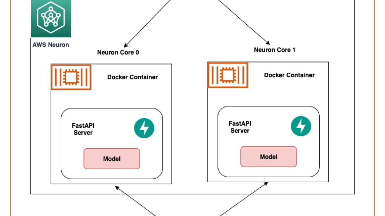
Ankur Srivastava is a Sr. Solutions Architect in the ML Frameworks Team. He focuses on helping customers with self-managed distributed training and inference at scale on AWS. His experience includes industrial predictive maintenance, digital twins, probabilistic design optimization and has completed his doctoral studies from Mechanical Engineering at Rice University and post-doctoral research from Massachusetts Institute of Technology.

K.C. Tung is a Senior Solution Architect in AWS Annapurna Labs. He specializes in large deep learning model training and deployment at scale in cloud. He has a Ph.D. in molecular biophysics from the University of Texas Southwestern Medical Center in Dallas. He has spoken at AWS Summits and AWS Reinvent. Today he helps customers to train and deploy large PyTorch and TensorFlow models in AWS cloud. He is the author of two books: Learn TensorFlow Enterprise and TensorFlow 2 Pocket Reference.

Pronoy Chopra is a Senior Solutions Architect with the Startups Generative AI team at AWS. He specializes in architecting and developing IoT and Machine Learning solutions. He has co-founded two startups in the past and enjoys being hands-on with projects in the IoT, AI/ML and Serverless domain.

Read More