Posts in category: Amazon AWS

Implementing a modern data architecture provides a scalable method to integrate data from disparate sources. By organizing data by business domains instead of infrastructure, each domain can choose tools that suit their needs. Organizations can maximize the value of their modern data architecture with generative AI solutions while innovating continuously.

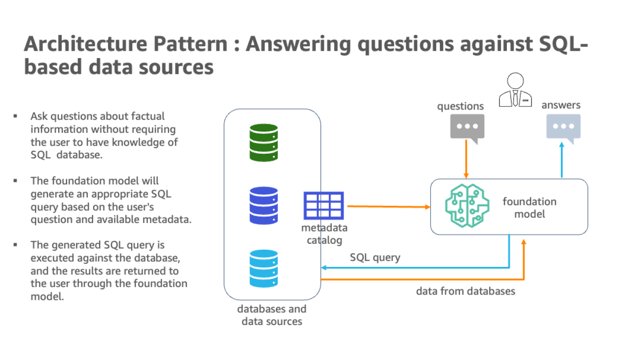
The natural language capabilities allow non-technical users to query data through conversational English rather than complex SQL. However, realizing the full benefits requires overcoming some challenges. The AI and language models must identify the appropriate data sources, generate effective SQL queries, and produce coherent responses with embedded results at scale. They also need a user interface for natural language questions.

Overall, implementing a modern data architecture and generative AI techniques with AWS is a promising approach for gleaning and disseminating key insights from diverse, expansive data at an enterprise scale. The latest offering for generative AI from AWS is Amazon Bedrock, which is a fully managed service and the easiest way to build and scale generative AI applications with foundation models. AWS also offers foundation models through Amazon SageMaker JumpStart as Amazon SageMaker endpoints. The combination of large language models (LLMs), including the ease of integration that Amazon Bedrock offers, and a scalable, domain-oriented data infrastructure positions this as an intelligent method of tapping into the abundant information held in various analytics databases and data lakes.

In the post, we showcase a scenario where a company has deployed a modern data architecture with data residing on multiple databases and APIs such as legal data on Amazon Simple Storage Service (Amazon S3), human resources on Amazon Relational Database Service (Amazon RDS), sales and marketing on Amazon Redshift, financial market data on a third-party data warehouse solution on Snowflake, and product data as an API. This implementation aims to enhance the productivity of the enterprise’s business analytics, product owners, and business domain experts. All this achieved through the use of generative AI in this domain mesh architecture, which enables the company to achieve its business objectives more efficiently. This solution has the option to include LLMs from JumpStart as a SageMaker endpoint as well as third-party models. We provide the enterprise users with a medium of asking fact-based questions without having an underlying knowledge of data channels, thereby abstracting the complexities of writing simple to complex SQL queries.

Solution overview

A modern data architecture on AWS applies artificial intelligence and natural language processing to query multiple analytics databases. By using services such as Amazon Redshift, Amazon RDS, Snowflake, Amazon Athena, and AWS Glue, it creates a scalable solution to integrate data from various sources. Using LangChain, a powerful library for working with LLMs, including foundation models from Amazon Bedrock and JumpStart in Amazon SageMaker Studio notebooks, a system is built where users can ask business questions in natural English and receive answers with data drawn from the relevant databases.

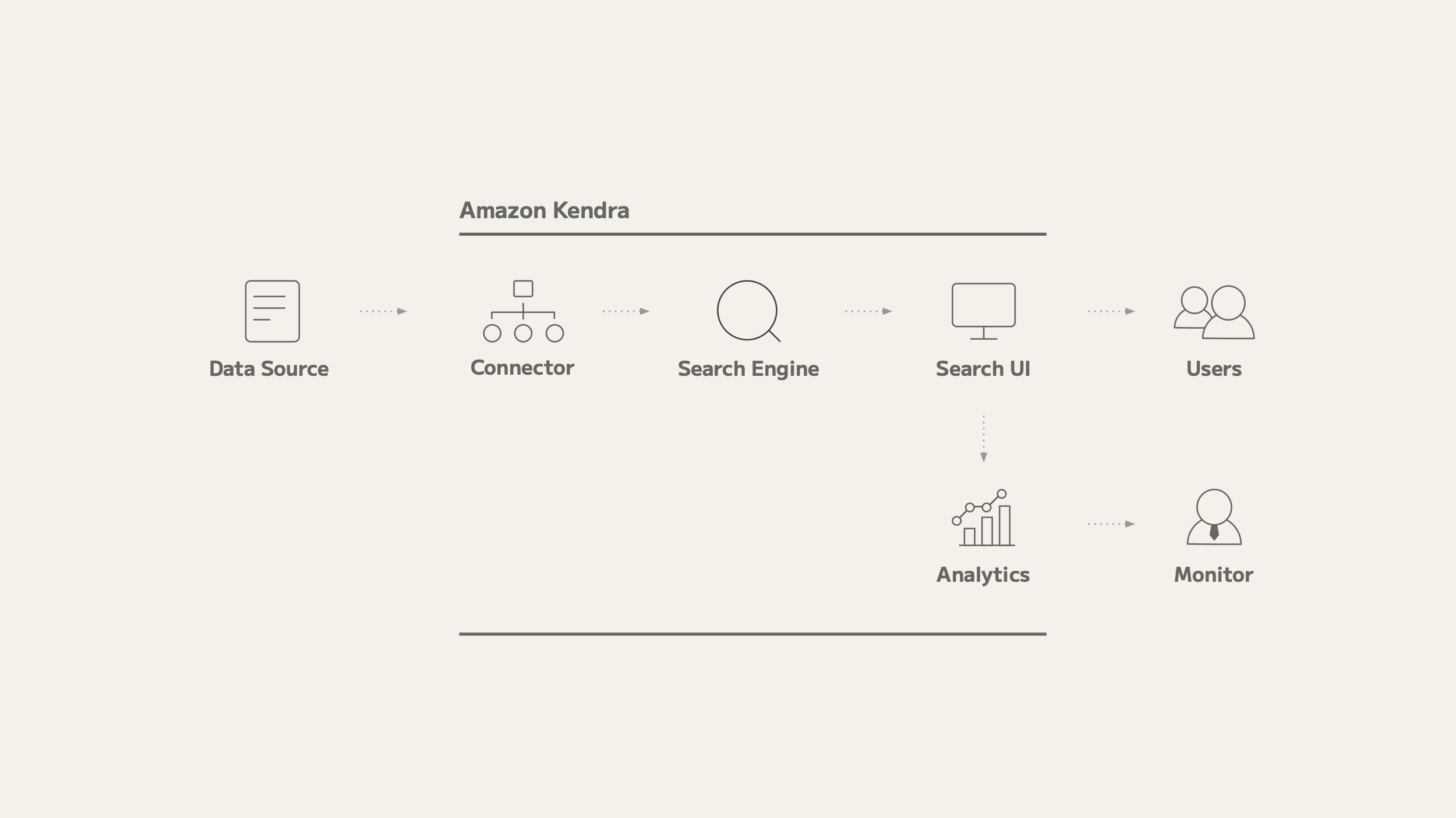
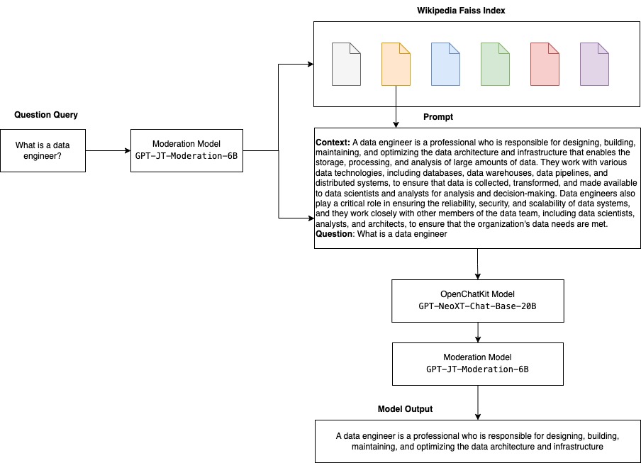
The following diagram illustrates the architecture.

The hybrid architecture uses multiple databases and LLMs, with foundation models from Amazon Bedrock and JumpStart for data source identification, SQL generation, and text generation with results.

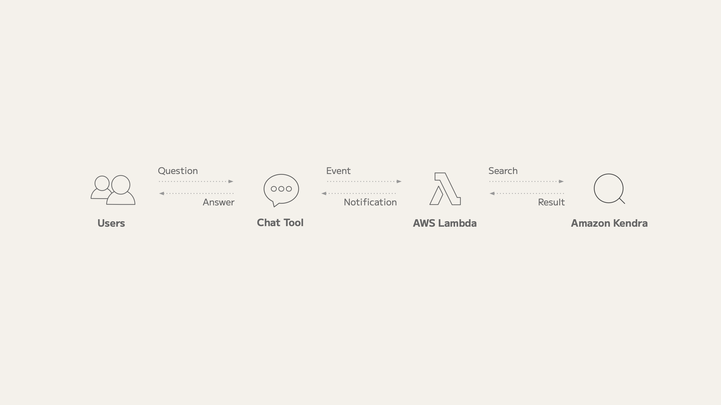
The following diagram illustrates the specific workflow steps for our solution.

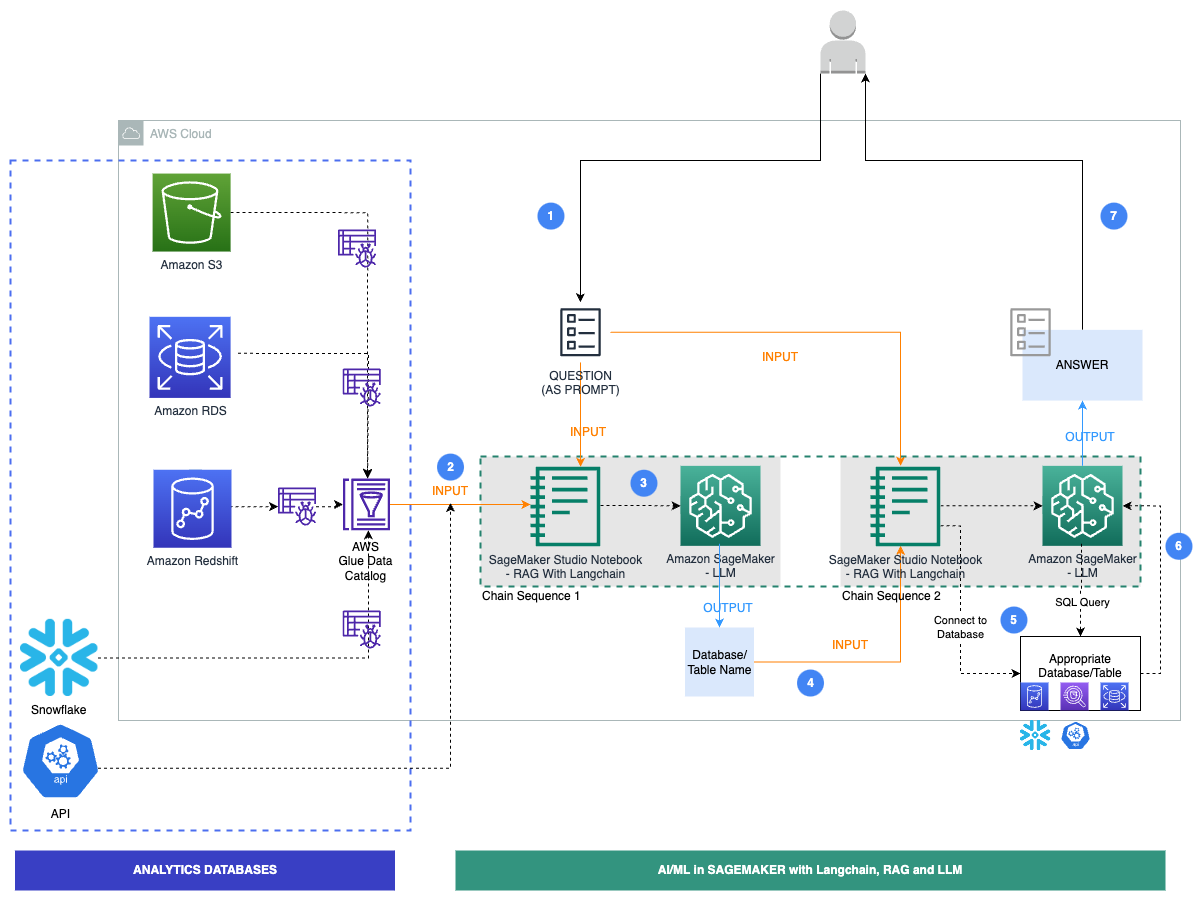
The steps are follows:

1. A business user provides an English question prompt.
2. An AWS Glue crawler is scheduled to run at frequent intervals to extract metadata from databases and create table definitions in the AWS Glue Data Catalog. The Data Catalog is input to Chain Sequence 1 (see the preceding diagram).
3. LangChain, a tool to work with LLMs and prompts, is used in Studio notebooks. LangChain requires an LLM to be defined. As part of Chain Sequence 1, the prompt and Data Catalog metadata are passed to an LLM, hosted on a SageMaker endpoint, to identify the relevant database and table using LangChain.
4. The prompt and identified database and table are passed to Chain Sequence 2.
5. LangChain establishes a connection to the database and runs the SQL query to get the results.
6. The results are passed to the LLM to generate an English answer with the data.
7. The user receives an English answer to their prompt, querying data from different databases.

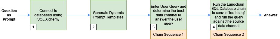
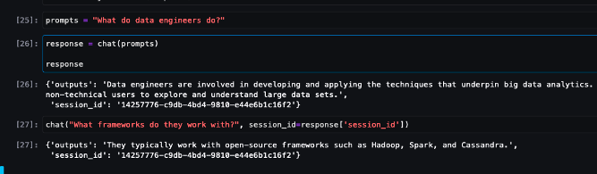
This following sections explain some of the key steps with associated code. To dive deeper into the solution and code for all steps shown here, refer to the GitHub repo. The following diagram shows the sequence of steps followed:

Prerequisites

You can use any databases that are compatible with SQLAlchemy to generate responses from LLMs and LangChain. However, these databases must have their metadata registered with the AWS Glue Data Catalog. Additionally, you will need to have access to LLMs through either JumpStart or API keys.

Connect to databases using SQLAlchemy

LangChain uses SQLAlchemy to connect to SQL databases. We initialize LangChain’s SQLDatabase function by creating an engine and establishing a connection for each data source. The following is a sample of how to connect to an Amazon Aurora MySQL-Compatible Edition serverless database and include only the employees table:

#connect to AWS Aurora MySQL
cluster_arn = <cluster_arn>
secret_arn = <secret_arn>
engine_rds=create_engine('mysql+auroradataapi://:@/employees',echo=True,
  connect_args=dict(aurora_cluster_arn=cluster_arn, secret_arn=secret_arn))
dbrds = SQLDatabase(engine_rds, include_tables=['employees'])

Next, we build prompts used by Chain Sequence 1 to identify the database and the table name based on the user question.

Generate dynamic prompt templates

We use the AWS Glue Data Catalog, which is designed to store and manage metadata information, to identify the source of data for a user query and build prompts for Chain Sequence 1, as detailed in the following steps:

1. We build a Data Catalog by crawling through the metadata of multiple data sources using the JDBC connection used in the demonstration.
2. With the Boto3 library, we build a consolidated view of the Data Catalog from multiple data sources. The following is a sample on how to get the metadata of the employees table from the Data Catalog for the Aurora MySQL database:

 #retrieve metadata from glue data catalog
  glue_tables_rds = glue_client.get_tables(DatabaseName=<database_name>, MaxResults=1000)
    for table in glue_tables_rds['TableList']:
        for column in table['StorageDescriptor']['Columns']:
             columns_str=columns_str+'n'+('rdsmysql|employees|'+table['Name']+"|"+column['Name'])

A consolidated Data Catalog has details on the data source, such as schema, table names, and column names. The following is a sample of the output of the consolidated Data Catalog:

database|schema|table|column_names
redshift|tickit|tickit_sales|listid
rdsmysql|employees|employees|emp_no
....
s3|none|claims|policy_id

3. We pass the consolidated Data Catalog to the prompt template and define the prompts used by LangChain:

prompt_template = """
From the table below, find the database (in column database) which will contain the data (in corresponding column_names) to answer the question {query} n
"""+glue_catalog +""" Give your answer as database == n Also,give your answer as database.table =="""

Chain Sequence 1: Detect source metadata for the user query using LangChain and an LLM

We pass the prompt template generated in the previous step to the prompt, along with the user query to the LangChain model, to find the best data source to answer the question. LangChain uses the LLM model of our choice to detect source metadata.

Use the following code to use an LLM from JumpStart or third-party models:

#define your LLM model here
llm = <LLM>
#pass prompt template and user query to the prompt
PROMPT = PromptTemplate(template=prompt_template, input_variables=["query"])
# define llm chain
llm_chain = LLMChain(prompt=PROMPT, llm=llm)
#run the query and save to generated texts
generated_texts = llm_chain.run(query)

The generated text contains information such as the database and table names against which the user query is run. For example, for the user query “Name all employees with birth date this month,” generated_text has the information database == rdsmysql and database.table == rdsmysql.employees.

Next, we pass the details of the human resources domain, Aurora MySQL database, and employees table to Chain Sequence 2.

Chain Sequence 2: Retrieve responses from the data sources to answer the user query

Next, we run LangChain’s SQL database chain to convert text to SQL and implicitly run the generated SQL against the database to retrieve the database results in a simple readable language.

We start with defining a prompt template that instructs the LLM to generate SQL in a syntactically correct dialect and then run it against the database:

_DEFAULT_TEMPLATE = """Given an input question, first create a syntactically correct {dialect} query to run, then look at the results of the query and return the answer.
Only use the following tables:
{table_info}
If someone asks for the sales, they really mean the tickit.sales table.
Question: {input}"""
#define the prompt
PROMPT = PromptTemplate( input_variables=["input", "table_info", "dialect"], template=_DEFAULT_TEMPLATE)

Finally, we pass the LLM, database connection, and prompt to the SQL database chain and run the SQL query:

db_chain = SQLDatabaseChain.from_llm(llm, db, prompt=PROMPT)
response=db_chain.run(query)

For example, for the user query “Name all employees with birth date this month,” the answer is as follows:

Question: Name all employees with birth date this month

SELECT * FROM employees WHERE MONTH(birth_date) = MONTH(CURRENT_DATE());

User Response:
The employees with birthdays this month are:
Christian Koblick
Tzvetan Zielinski

Clean up

After you run the modern data architecture with generative AI, make sure to clean up any resources that won’t be utilized. Shut down and delete the databases used (Amazon Redshift, Amazon RDS, Snowflake). In addition, delete the data in Amazon S3 and stop any Studio notebook instances to not incur any further charges. If you used JumpStart to deploy an LLM as a SageMaker real-time endpoint, delete endpoint through either the SageMaker console or Studio.

Conclusion

In this post, we integrated a modern data architecture with generative AI and LLMs within SageMaker. This solution uses various text-to-text foundation models from JumpStart as well as third-party models. This hybrid approach identifies data sources, writes SQL queries, and generates responses with query results. It uses Amazon Redshift, Amazon RDS, Snowflake, and LLMs. To improve the solution, you could add more databases, a UI for English queries, prompt engineering, and data tools. This could become an intelligent, unified way to get insights from multiple data stores. To dive deeper into the solution and the code shown in this post, check out the GitHub repo . Also, refer to Amazon Bedrock for use cases on generative AI, foundation models, and large language models.

Appendix

Example prompts

About the Authors

Navneet Tuteja is a Data Specialist at Amazon Web Services. Before joining AWS, Navneet worked as a facilitator for organizations seeking to modernize their data architectures and implement comprehensive AI/ML solutions. She holds an engineering degree from Thapar University, as well as a master’s degree in statistics from Texas A&M University.

Sovik Kumar Nath is an AI/ML solution architect with AWS. He has extensive experience designing end-to-end machine learning and business analytics solutions in finance, operations, marketing, healthcare, supply chain management, and IoT. Sovik has published articles and holds a patent in ML model monitoring. He has double masters degrees from the University of South Florida, University of Fribourg, Switzerland, and a bachelors degree from the Indian Institute of Technology, Kharagpur. Outside of work, Sovik enjoys traveling, taking ferry rides, and watching movies.

Read More

This is a guest post by Dr. Naoki Okada, Lead Data Scientist at BrainPad Inc.

Founded in 2004, BrainPad Inc. is a pioneering partner in the field of data utilization, helping companies create business and improve their management through the use of data. To date, BrainPad has helped more than 1,300 companies, primarily industry leaders. BrainPad has the advantage of providing a one-stop service from formulating a data utilization strategy to proof of concept and implementation. BrainPad’s unique style is to work together with clients to solve problems on the ground, such as data that isn’t being collected due to a siloed organizational structure or data that exists but isn’t organized.

This post discusses how to structure internal knowledge sharing using Amazon Kendra and AWS Lambda and how Amazon Kendra solves the obstacles around knowledge sharing many companies face. We summarize BrainPad’s efforts in four key areas:

• What are the knowledge sharing problems that many companies face?
• Why did we choose Amazon Kendra?
• How did we implement the knowledge sharing system?
• Even if a tool is useful, it is meaningless if it is not used. How did we overcome the barrier to adoption?

Knowledge sharing problems that many companies face

Many companies achieve their results by dividing their work into different areas. Each of these activities generates new ideas every day. This knowledge is accumulated on an individual basis. If this knowledge can be shared among people and organizations, synergies in related work can be created, and the efficiency and quality of work will increase dramatically. This is the power of knowledge sharing.

However, there are many common barriers to knowledge sharing:

• Few people are proactively involved, and the process can’t be sustained for long due to busy schedules.
• Knowledge is scattered across multiple media, such as internal wikis and PDFs, making it difficult to find the information you need.
• No one enters knowledge into the knowledge consolidation system. The system will not be widely used because of its poor searchability.

Our company faced a similar situation. The fundamental problem with knowledge sharing is that although most employees have a strong need to obtain knowledge, they have little motivation to share their own knowledge at a cost. Changing employee behavior for the sole purpose of knowledge sharing is not easy.

In addition, each employee or department has its own preferred method of accumulating knowledge, and trying to force unification won’t lead to motivation or performance in knowledge sharing. This is a headache for management, who wants to consolidate knowledge, while those in the field want to have knowledge in a decentralized way.

At our company, Amazon Kendra is the cloud service that has solved these problems.

Why we chose Amazon Kendra

Amazon Kendra is a cloud service that allows us to search for internal information from a common interface. In other words, it is a search engine that specializes in internal information. In this section, we discuss the three key reasons why we chose Amazon Kendra.

Easy aggregation of knowledge

As mentioned in the previous section, knowledge, even when it exists, tends to be scattered across multiple media. In our case, it was scattered across our internal wiki and various document files. Amazon Kendra provides powerful connectors for this situation. We can easily import documents from a variety of media, including groupware, wikis, Microsoft PowerPoint files, PDFs, and more, without any hassle.

This means that employees don’t have to change the way they store knowledge in order to share it. Although knowledge aggregation can be achieved temporarily, it’s very costly to maintain. The ability to automate this was a very desirable factor for us.

Great searchability

There are a lot of groupware and wikis out there that excel at information input. However, they often have weaknesses in information output (searchability). This is especially true for Japanese search. For example, in English, word-level matching provides a reasonable level of searchability. In Japanese, however, word extraction is more difficult, and there are cases where matching is done by separating words by an appropriate number of characters. If a search for “Tokyo-to (東京都)” is separated by two characters, “Tokyo (東京)” and “Kyoto (京都),” it will be difficult to find the knowledge you are looking for.

Amazon Kendra offers great searchability through machine learning. In addition to traditional keyword searches such as “technology trends,” natural language searches such as “I want information on new technology initiatives” can greatly enhance the user experience. The ability to search appropriately for collected information is the second reason we chose Amazon Kendra.

Low cost of ownership

IT tools that specialize in knowledge aggregation and retrieval are called enterprise search systems. One problem with implementing these systems is the cost. For an organization with several hundred employees, operating costs can exceed 10 million yen per year. This is not a cheap way to start a knowledge sharing initiative.

Amazon Kendra is offered at a much lower cost than most enterprise search systems. As mentioned earlier, knowledge sharing initiatives are not easy to implement. We wanted to start small, and Amazon Kendra’s low cost of ownership was a key factor in our decision.

In addition, Amazon Kendra’s ease of implementation and flexibility are also great advantages for us. The next section summarizes an example of our implementation.

How we implemented the knowledge sharing system

Implementation is not an exaggerated development process; it can be done without code by following the Amazon Kendra processing flow. Here are five key points in the implementation process:

• Data source (accumulating knowledge) – Each department and employee of our company frequently held internal study sessions, and through these activities, knowledge was accumulated in multiple media, such as wikis and various types of storage. At that time, it was easy to review the information from the study sessions later. However, in order to extract knowledge about a specific area or technology, it was necessary to review each medium in detail, which was not very convenient.
• Connectors (aggregating knowledge) – With the connector functionality in Amazon Kendra, we were able to link knowledge scattered throughout the company into Amazon Kendra and achieve cross-sectional searchability. In addition, the connector is loaded through a restricted account, allowing for a security-conscious implementation.
• Search engine (finding information) – Because Amazon Kendra has a search page for usability testing, we were able to quickly test the usability of the search engine immediately after loading documents to see what kind of knowledge could be found. This was very helpful in solidifying the image of the launch.
• Search UI (search page for users) – Amazon Kendra has a feature called Experience Builder that exposes the search screen to users. This feature can be implemented with no code, which was very helpful in getting feedback during the test deployment. In addition to Experience Builder, Amazon Kendra also supports Python and React.js API implementations, so we can eventually provide customized search pages to our employees to improve their experience.
• Analytics (monitoring usage trends) – An enterprise search system is only valuable if a lot of people are using it. Amazon Kendra has the ability to monitor how many searches are being performed and for what terms. We use this feature to track usage trends.

We also have some Q&A related to our implementation:

• What were some of the challenges in gathering internal knowledge? We had to start by collecting the knowledge that each department and employee had, but not necessarily in a place that could be directly connected to Amazon Kendra.
• How did we benefit from Amazon Kendra? We had tried to share knowledge many times in the past, but had often failed. The reasons were information aggregation, searchability, operational costs, and implementation costs. Amazon Kendra has features that solve these problems, and we successfully launched it within about 3 months of conception. Now we can use Amazon Kendra to find solutions to tasks that previously required the knowledge of individuals or departments as the collective knowledge of the entire organization.
• How did you evaluate the searchability of the system, and what did you do to improve it? First, we had many employees interact with the system and get feedback. One problem that arose at the beginning of the implementation was that there was a scattering of information that had little value as knowledge. This was because some of the data sources contained information from internal blog posts, for example. We are continually working to improve the user experience by selecting the right data sources.

As mentioned earlier, by using Amazon Kendra, we were able to overcome many implementation hurdles at minimal cost. However, the biggest challenge with this type of tool is the adoption barrier that comes after implementation. The next section provides an example of how we overcame this hurdle.

How we overcame the barrier to adoption

Have you ever seen a tool that you spent a lot of effort, time, and money implementing become obsolete without widespread use? No matter how good the functionality is at solving problems, it will not be effective if people are not using it.

One of the initiatives we took with the launch of Amazon Kendra was to provide a chatbot. In other words, when you ask a question in a chat tool, you get a response with the appropriate knowledge. Because all of our telecommuting employees use a chat tool on a daily basis, using chatbots is much more compatible than having them open a new search screen in their browsers.

To implement this chatbot, we use Lambda, a service that allows us to run serverless, event-driven programs. Specifically, the following workflow is implemented:

1. A user posts a question to the chatbot with a mention.
2. The chatbot issues an event to Lambda.
3. A Lambda function detects the event and searches Amazon Kendra for the question.
4. The Lambda function posts the search results to the chat tool.
5. The user views the search results.

This process takes only a few seconds and provides a high-quality user experience for knowledge discovery. The majority of employees were exposed to the knowledge sharing mechanism through the chatbot, and there is no doubt that the chatbot contributed to the diffusion of the mechanism. And because there are some areas that can’t be covered by the chatbot alone, we have also asked them to use the customized search screen in conjunction with the chatbot to provide an even better user experience.

Conclusion

In this post, we presented a case study of Amazon Kendra for knowledge sharing and an example of a chatbot implementation using Lambda to propagate the mechanism. We look forward to seeing Amazon Kendra take another leap forward as large-scale language models continue to evolve.

If you are interested in trying out Amazon Kendra, check out Enhancing enterprise search with Amazon Kendra. BrainPad can also help you with internal knowledge sharing and document exploitation using generative AI. Please contact us for more information.

About the Author

Dr. Naoki Okada is a Lead Data Scientist at BrainPad Inc. With his cross-functional experience in business, analytics, and engineering, he supports a wide range of clients from building up DX organizations to leveraging data in unexplored areas.

Read More

The size of the machine learning (ML) models––large language models (LLMs) and foundation models (FMs)––is growing fast year-over-year, and these models need faster and more powerful accelerators, especially for generative AI. AWS Inferentia2 was designed from the ground up to deliver higher performance while lowering the cost of LLMs and generative AI inference.

In this post, we show how the second generation of AWS Inferentia builds on the capabilities introduced with AWS Inferentia1 and meets the unique demands of deploying and running LLMs and FMs.

The first generation of AWS Inferentia, a purpose-built accelerator launched in 2019, is optimized to accelerate deep learning inference. AWS Inferentia helped ML users reduce their inference costs and improve their prediction throughput and latency. With AWS Inferentia1, customers saw up to 2.3x higher throughput and up to 70% lower cost per inference than comparable inference-optimized Amazon Elastic Compute Cloud (Amazon EC2) instances.

AWS Inferentia2, featured in the new Amazon EC2 Inf2 instances and supported in Amazon SageMaker, is optimized for large-scale generative AI inference and is the first inference focused instance from AWS that is optimized for distributed inference, with high-speed, low-latency connectivity between accelerators.

You can now efficiently deploy a 175-billion-parameter model for inference across multiple accelerators on a single Inf2 instance without requiring expensive training instances. Until now, customers who had large models could only use instances that were built for training, but this is a waste of resources––given that they’re more expensive, consume more energy, and their workload doesn’t make use of all the available resources (such as faster networking and storage). With AWS Inferentia2, you can achieve 4 times higher throughput and up to 10 times lower latency compared to AWS Inferentia1. Also, the second generation of AWS Inferentia adds enhanced support for more data types, custom operators, dynamic tensors, and more.

AWS Inferentia2 has 4 times more memory capacity, 16.4 times higher memory bandwidth than AWS Inferentia1, and native support for sharding large models across multiple accelerators. The accelerators use NeuronLink and Neuron Collective Communication to maximize the speed of data transfer between them or between an accelerator and the network adapter. AWS Inferentia2 is better suited for larger models, which require sharding across multiple accelerators, although AWS Inferentia1 is still a great option for smaller models because it provides better price-performance compared to alternatives.

Architecture evolution

To compare both generations of AWS Inferentia, let’s review the architecture of AWS Inferentia1. It has four NeuronCores v1 per chip, shown in the following diagram.

Specifications per chip:

• Compute – Four cores delivering in total 128 INT8 TOPS and 64FP16/BF16 TFLOPS
• Memory – 8 GB of DRAM (50 GB/sec of bandwidth), shared by all four cores
• NeuronLink – Link between cores for sharding models across two or more cores

Let’s look at how AWS Inferentia2 is organized. Each AWS Inferentia2 chip has two upgraded cores based on the NeuronCore-v2 architecture. Like AWS Inferentia1, you can run different models on each NeuronCore or combine multiple cores to shard big models.

Specifications per chip:

• Compute – Two cores delivering in total 380 INT8 TOPS, 190 FP16/BF16/cFP8/TF32 TFLOPS, and 47.5 FP32 TFLOPS
• Memory – 32 GB of HBM, shared by both cores
• NeuronLink – Link between chips (384 GB/sec per device) for sharding models across two or more cores

NeuronCore-v2 has a modular design with four independent engines:

• ScalarEngine (3 times faster than v1) – Operates on floating point numbers––1600 (BF16/FP16) FLOPS
• VectorEngine (10 times faster than v1) – Operates on vectors of numbers with single operation for computations such as normalization, pooling, and others.
• TensorEngine (6 times faster than v1) – Performs tensor computations such as Conv, Reshape, Transpose, and others.
• GPSIMD-Engine – Has eight fully programmable 512-bit wide general-purpose processors for you to create your custom operators with standard PyTorch custom C++ operators API. This is a new feature, introduced in NeuronCore-v2.

AWS Inferentia2 NeuronCore-v2 is faster and more optimized. Also, it’s capable of accelerating different types and sizes of models, ranging from simple models such as ResNet 50 to large language models or foundation models with billions of parameters such as GPT-3 (175 billion parameters). AWS Inferentia2 also has a larger and faster internal memory, when compared to AWS Inferentia1, as shown in the following table.

The memory you find in AWS Inferentia2 is the type High-Bandwidth Memory (HBM) type. Each AWS Inferentia2 chip has 32 GB and that can be combined with other chips to distribute very large models using NeuronLink (device-to-device interconnect). An inf2.48xlarge, for instance, has 12 AWS Inferentia2 accelerators with a total of 384 GB of accelerated memory. The speed of AWS Inferentia2 memory is 16.4 times faster than AWS Inferentia1, as shown in the previous table.

Other features

AWS Inferentia2 offers the following additional features:

• Hardware supported – cFP8 (new, configurable FP8), FP16, BF16, TF32, FP32, INT8, INT16 and INT32. For more information, refer to Data Types.
• Lazy Tensor inference – We discuss Lazy Tensor inference later in this post.
• Custom operators – Developers can use standard PyTorch custom operators programming interfaces to use the Custom C++ Operators feature. A custom operator is composed of low-level primitives available in the Tensor Factory Functions and accelerated by GPSIMD-Engine.
• Control-flow (coming soon) – This is for native programming language control flow inside the model to eventually preprocess and postprocess data from one layer to another.
• Dynamic-shapes (coming soon) – This is useful when your model changes the shape of the output of any internal layer dynamically. For instance: a filter which reduces the output tensor size or shape inside the model, based on the input data.

Accelerating models on AWS Inferentia1 and AWS Inferentia2

The AWS Neuron SDK is used for compiling and running your model. It is natively integrated with PyTorch and TensorFlow. That way, you don’t need to run an additional tool. Use your original code, written in one of these ML frameworks, and with a few lines of code changes, you’re good to go with AWS Inferentia.

Let’s look at how to compile and run a model on AWS Inferentia1 and AWS Inferentia2 using PyTorch.

Load a pre-trained model (ResNet 50) from torchvision

Load a pre-trained model and run it one time to warm it up:

import torch
import torchvision

model = torchvision.models.resnet50(weights='IMAGENET1K_V1').eval().cpu()
x = torch.rand(1,3,224,224).float().cpu() # dummy input
y = model(x) # warmup model

Trace and deploy the accelerated model on Inferentia1

To trace the model to AWS Inferentia, import torch_neuron and invoke the tracing function. Keep in mind that the model needs to be PyTorch Jit traceable to work.

At the end of the tracing process, save the model as a normal PyTorch model. Compile the model one time and load it back as many times as you need. The Neuron SDK runtime is already integrated to PyTorch and is responsible for sending the operators to the AWS Inferentia1 chip automatically to accelerate your model.

In your inference code, you always need to import torch_neuron to activate the integrated runtime.

You can pass additional parameters to the compiler to customize the way it optimizes the model or to enable special features such as neuron-pipeline-cores. Shard your model across multiple cores to increase throughput.

import torch_neuron

# Tracing the model using AWS NeuronSDK
neuron_model = torch_neuron.trace(model,x) # trace model to Inferentia
# Saving for future use
neuron_model.save('neuron_resnet50.pt')

# Next time you don't need to trace the model again
# Just load it and AWS NeuronSDK will send it to Inferentia automatically
neuron_model = torch.jit.load('neuron_resnet50.pt')

# accelerated inference on Inferentia
y = neuron_model(x)

Tracing and deploying the accelerated model on Inferentia2

For AWS Inferentia2, the process is similar. The only difference is the package you import ends with x: torch_neuronx. The Neuron SDK takes care of the compilation and running of the model for you transparently. You can also pass additional parameters to the compiler to fine-tune the operation or activate specific functionalities.

import torch_neuronx

# Tracing the model using NeuronSDK
neuron_model = torch_neuronx.trace(model,x) # trace model to Inferentia
# Saving for future use
neuron_model.save('neuron_resnet50.pt')

# Next time you don't need to trace the model again
# Just load it and NeuronSDK will send it to Inferentia automatically
neuron_model = torch.jit.load('neuron_resnet50.pt')

# accelerated inference on Inferentia
y = neuron_model(x)

AWS Inferentia2 also offers a second approach for running a model called Lazy Tensor inference. In this mode, you don’t trace or compile the model previously; instead, the compiler runs on the fly every time you run your code. It isn’t recommended for production, given that traced mode has many advantages over Lazy Tensor inference. However, if you’re still developing your model and need to test it faster, Lazy Tensor inference can be a good alternative. Here’s how to compile and run a model using Lazy Tensor:

import torch
import torchvision
import torch_neuronx
import torch_xla.core.xla_model as xm

device = xm.xla_device() # Create XLA device
model = torchvision.models.resnet50(weights='IMAGENET1K_V1').eval().cpu()
model.to(device)

x = torch.rand((1,3,224,224), device=device) # dummy input
with torch.no_grad():
  y = model(x)
  xm.mark_step() # Compilation occurs here

Now that you’re familiar with AWS Inferentia2, a good next step is to get started with PyTorch or Tensorflow and learn how to set up a dev environment and run tutorials and examples. Also, check the AWS Neuron Samples GitHub repo, where you can find multiple examples of how to prepare models to run on Inf2, Inf1, and Trn1.

Summary of feature comparison between AWS Inferentia1 and AWS Inferentia2

The AWS Inferentia2 compiler is XLA-based, and AWS is part of OpenXLA initiative. This is the biggest difference over AWS Inferentia1, and that’s relevant because PyTorch, TensorFlow, and JAX have native XLA integrations. XLA brings many performance improvements, given that it optimizes the graph to compute the results in a single kernel launch. It fuses together successive tensor operations and outputs optimal machine code for accelerating model runs on AWS Inferentia2. Other parts of the Neuron SDK were also improved in AWS Inferentia2, while keeping the user experience as simple as possible while tracing and running models. The following table shows the features available in both versions of the compiler and runtime.

For a more detailed comparison between torch-neuron (Inf1) and torch-neuronx (Inf2), refer to Comparison of torch-neuron (Inf1) versus torch-neuronx (Inf2 & Trn1) for Inference.

Model Serving

After tracing a model to deploy to Inf2, you have many deployment options. You can run real-time predictions or batch predictions in different ways. Inf2 is available because EC2 instances are natively integrated to other AWS services that make use of Deep Learning Containers (DLCs) such as Amazon Elastic Container Service (Amazon ECS), Amazon Elastic Kubernetes Service (Amazon EKS), and SageMaker.

AWS Inferentia2 is compatible with the most popular deployment technologies. Here are a list of some of the options you have for deploying models using AWS Inferentia2:

• SageMaker – Fully managed service to prepare data and build, train, and deploy ML models
• TorchServe – PyTorch integrated deployment mechanism
• TensorFlow Serving – TensorFlow integrated deployment mechanism
• Deep Java Library – Open-source Java mechanism for model deployment and training
• Triton – NVIDIA open-source service for model deployment

Benchmark

The following table highlights the improvements AWS Inferentia2 brings over AWS Inferentia1. Specifically, we measure latency (how fast the model can make a prediction using each accelerator), throughput (how many inferences per second), and cost per inference (how much each inference costs in US dollars). The lower the latency in milliseconds and costs in US dollars, the better. The higher the throughput the better.

Two models were used in this process––both large language models: ELECTRA large discriminator and BERT large uncased. PyTorch (1.13.1) and Hugging Face transformers (v4.7.0), the main libraries used in this experiment, ran on Python 3.8. After compiling the models for batch size = 1 and 10 (using the code from the previous section as a reference), each model was warmed up (invoked one time to initialize the context) and then invoked 10 times in a row. The following table shows average numbers collected in this simple benchmark.

• Electra large discriminator (334,092,288 parameters ~593 MB)
• Bert large uncased (335,143,938 parameters ~580 MB)
• OPT-66B (66 billion parameterss ~124 GB)

* c6a.8xlarge with 32 AMD Epyc 7313 CPU was used in this benchmark.

**EC2 Public pricing in us-east-1 on April 20: inf2.xlarge: $0.7582/hr; inf1.xlarge: $0.228/hr. Cost per inference considers the cost per element in a batch. (Cost per inference equals the total cost of model invocation/batch size.)

For additional information about training and inference performance, refer to Trn1/Trn1n Performance.

Conclusion

AWS Inferentia2 is a powerful technology designed for improving performance and reducing costs of deep learning model inference. More performant than AWS Inferentia1, it offers up to 4 times higher throughput, up to 10 times lower latency, and up to 50% better performance/watt than other comparable inference-optimized EC2 instances. In the end, you pay less, have a faster application, and meet your sustainability goals.

It’s simple and straightforward to migrate your inference code to AWS Inferentia2, which also supports a broader variety of models, including large language models and foundation models for generative AI.

You can get started by following the AWS Neuron SDK documentation to set up a development environment and start your accelerated deep learning project. To help you get started, Hugging Face has added Neuron support to their Optimum library, which optimizes models for faster training and inference, and they have many examples tasks ready to run on Inf2. Also, check our Deploy large language models on AWS Inferentia2 using large model inference containers to learn about deploying LLMs to AWS Inferentia2 using model inference containers. For additional examples, see the AWS Neuron Samples GitHub repo.

About the authors

Samir Araújo is an AI/ML Solutions Architect at AWS. He helps customers creating AI/ML solutions which solve their business challenges using AWS. He has been working on several AI/ML projects related to computer vision, natural language processing, forecasting, ML at the edge, and more. He likes playing with hardware and automation projects in his free time, and he has a particular interest for robotics.

Read More

Last week, Technology Innovation Institute (TII) launched TII Falcon LLM, an open-source foundational large language model (LLM). Trained on 1 trillion tokens with Amazon SageMaker, Falcon boasts top-notch performance (#1 on the Hugging Face leaderboard at time of writing) while being comparatively lightweight and less expensive to host than other LLMs such as llama-65B. In this post, we demonstrate how to deploy Falcon for applications like language understanding and automated writing assistance using large model inference deep learning containers on SageMaker.

The Falcon has landed on SageMaker

TII is the applied research organization within Abu Dhabi’s Advanced Technology Research Council; its team of scientists, researchers, and engineers is dedicated to the discovery of transformative technologies and development of scientific breakthroughs that will future-proof our society. Earlier this year, TII set out to train a state-of-the-art, open-source LLM and used the infrastructure, tooling, and expertise of SageMaker to get the job done (to learn more about how this model was trained on SageMaker, refer to Technology Innovation Institute trains the state-of-the-art Falcon LLM 40B foundation model on Amazon SageMaker). The result of this effort is TII Falcon LLM.

Trained on 1 trillion tokens, Falcon boasts top-notch performance against the Eleuther AI Language Model Evaluation Harness and is currently #1 on the Hugging Face leaderboard for accuracy. The model is available in two different sizes—Falcon-40B and Falcon-7B—and can be used for state-of-the-art performance in applications such as language understanding, conversational experiences, and automated writing assistance. This post will help you get started with deploying Falcon on SageMaker for high-accuracy inference in these types of domains.

SageMaker large model inference DLCs simplify LLM hosting

Hosting LLMs such as Falcon-40B and Falcon-7B can be challenging. Larger models are often more accurate because they include billions of parameters, but their size can also result in slower inference latency or worse throughput. Hosting an LLM can require more GPU memory and optimized kernels to achieve acceptable performance. To further complicate things, although smaller models such as Falcon-7B can generally fit on a single GPU such as an NVIDIA A10G instance that powers AWS G5 instance types, larger models like Falcon-40B cannot. When this happens, strategies such as tensor parallelism must be used to shard that larger model into multiple pieces and take advantage of the memory of multiple GPUs. Legacy hosting solutions used for smaller models typically don’t offer this type of functionality, adding to the difficulty.

SageMaker large model inference (LMI) deep learning containers (DLCs) can help. LMI DLCs are a complete end-to-end solution for hosting LLMs like Falcon-40B. At the front end, they include a high-performance model server (DJL Serving) designed for large model inference with features such as token streaming and automatic model replication within an instance to increase throughput. On the backend, LMI DLCs also include several high-performance model parallel engines, such as DeepSpeed and FasterTransformer, that can shard and manage model parameters across multiple GPUs. These engines also include optimized kernels for popular transformer models, which can accelerate inference by up to three times faster. With LMI DLCs, you simply need to create a configuration file to get started with LLM hosting on SageMaker. To learn more about SageMaker LMI DLCs, refer to Model parallelism and large model inference and our list of available images. You can also check out our previous post about hosting Bloom-175B on SageMaker using LMI DLCs.

Solution overview

This post walks you through how to host Falcon-40B using DeepSpeed on SageMaker using LMI DLCs. Falcon-40B requires that we use multiple A10 GPUs, whereas Falcon-7B only requires a single GPU. We have also prepared examples you can reference to host Falcon-40B and Falcon-7B using both DeepSpeed and Accelerate. You can find our code examples on GitHub.

This example can be run in SageMaker notebook instances or Amazon SageMaker Studio notebooks. For hosting Falcon-40B using LMI and DeepSpeed, we need to use an ml.g5.24xlarge instance. These instances provide 4x NVIDIA A10G GPUs, which each support 96 GiB of GPU memory. In addition, the host provides 96 vCPUs and 384 GiB of host memory. The LMI container will help address much of the undifferentiated heavy lifting associated with hosting LLMs, including downloading the model and partitioning the model artifact so that its comprising parameters can be spread across multiple GPUs.

Quotas for SageMaker machine learning (ML) instances can vary between accounts. If you receive an error indicating you’ve exceeded your quota for g5.24xlarge instances while following this post, you can increase the limit through the Service Quotas console.

Notebook walkthrough

To begin, we start by installing and importing the necessary dependencies for our example. We use the Boto3 SDK as well as the SageMaker SDK. Note that we use Amazon Simple Storage Service (Amazon S3) to store the model artifacts that we need for SageMaker and LMI to use, so we set up an S3 prefix variable accordingly. See the following code:

import sagemaker
import jinja2
from sagemaker import image_uris
import boto3
import os
import time
import json
from pathlib import Path
from sagemaker.utils import name_from_base

role = sagemaker.get_execution_role()  # execution role for the endpoint
sess = sagemaker.session.Session()  # sagemaker session for interacting with different AWS APIs
bucket = sess.default_bucket()  # bucket to house artifacts
model_bucket = sess.default_bucket()  # bucket to house artifacts
s3_code_prefix_deepspeed = "hf-large-model-djl-/code_falcon40b/deepspeed"  # folder within bucket where code artifact will go
region = sess._region_name
account_id = sess.account_id()
s3_client = boto3.client("s3")
sm_client = boto3.client("sagemaker")
smr_client = boto3.client("sagemaker-runtime")
jinja_env = jinja2.Environment()

We then create a local folder for our workspace to store our model artifacts:

!mkdir -p code_falcon40b_deepspeed

We first create a serving.properties configuration file in the local directory we created. This serving.properties file indicates to the LMI container and the front-end DJL Serving library which model parallelization and inference optimization engine we want to use. You can find the configuration options for both DeepSpeed and Hugging Face Accelerate in Configurations and settings. Here, note that we set the option.model_id parameter to define which Hugging Face model to pull from. SageMaker makes working with Hugging Face models simple, and this one line is all you need. In addition, we set option.tensor_parallel_degree to a value of 4 because we have four GPUs on our ml.g5.24xlarge instance. This parameter defines how many partitions of the model to create and distribute. Note that if we had used a larger instance with eight GPUs, such as ml.g5.48xlarge, and still set a value of 4, then LMI would automatically create two replicas of the model (two replicas spread across four GPUs each). See the following code:

%%writefile ./code_falcon40b_deepspeed/serving.properties
engine=Python
#to deploy falcon-40b-instruct set the model_id value to 'tiiuae/falcon-40b-instruct'
option.model_id=tiiuae/falcon-40b
option.tensor_parallel_degree=4
#option.s3url = {{s3url}}

You can also swap out tiiuae/falcon-40b with tiiuae/falcon-40b-instruct if it suits your needs better.

We also include a requirements.txt file that you can specify to install packages that you require:

%%writefile ./code_falcon40b_deepspeed/requirements.txt
einops
torch==2.0.1

The last thing we need is the model.py file that will be used with your model:

%%writefile ./code_falcon40b_deepspeed/model.py
from djl_python import Input, Output
import os
import torch
from transformers import pipeline, AutoModelForCausalLM, AutoTokenizer
from typing import Any, Dict, Tuple
import warnings

predictor = None


def get_model(properties):
    model_name = properties["model_id"]
    local_rank = int(os.getenv("LOCAL_RANK", "0"))
    model = AutoModelForCausalLM.from_pretrained(
        model_name,
        low_cpu_mem_usage=True,
        trust_remote_code=True,
        torch_dtype=torch.bfloat16,
        device_map="auto",
    )
    tokenizer = AutoTokenizer.from_pretrained(model_name)
    generator = pipeline(
        task="text-generation", model=model, tokenizer=tokenizer, device_map="auto"
    )
    return generator


def handle(inputs: Input) -> None:
    global predictor
    if not predictor:
        predictor = get_model(inputs.get_properties())
    if inputs.is_empty():
        # Model server makes an empty call to warmup the model on startup
        return None
    data = inputs.get_as_json()
    text = data["text"]
    text_length = data["text_length"]
    outputs = predictor(text, do_sample=True, min_length=text_length, max_length=text_length)
    result = {"outputs": outputs}
    return Output().add_as_json(result)

That’s it! At this point, we have created all the artifacts you will need deploy Falcon-40B with DeepSpeed! We package the directory into a *.tar.gz file and upload it to Amazon S3. Note that the actual model has not been downloaded or packaged into this file. The LMI container will download the model for you from Hugging Face directly. You also have the option to target an S3 bucket if you would like your own copy of the model in a location that will be more performant to download. LMI also includes optimization for downloading from Amazon S3 with high performance. See the following code:

s3_code_artifact_deepspeed= sess.upload_data("model.tar.gz", bucket, s3_code_prefix_deepspeed)
print(f"S3 Code or Model tar for deepspeed uploaded to --- > {s3_code_artifact_deepspeed}")

All that is left to do at this point is to define the container we want to use and create a model object:

inference_image_uri = (
    f"763104351884.dkr.ecr.{region}.amazonaws.com/djl-inference:0.22.1-deepspeed0.8.3-cu118"
)
model_name_acc = name_from_base(f"falcon40b-model-ds")
create_model_response = sm_client.create_model(
    ModelName=model_name_acc,
    ExecutionRoleArn=role,
    PrimaryContainer={"Image": inference_image_uri, "ModelDataUrl": s3_code_artifact_deepspeed},
)
model_arn = create_model_response["ModelArn"]

Then we create an endpoint configuration and create the endpoint:

endpoint_config_name = f"{model_name}-config"
endpoint_name = f"{model_name}-endpoint"
endpoint_config_response = sm_client.create_endpoint_config(
    EndpointConfigName=endpoint_config_name,
    ProductionVariants=[
        {
            "VariantName": "variant1",
            "ModelName": model_name,
            "InstanceType": "ml.g5.24xlarge",
            "InitialInstanceCount": 1,
            "ModelDataDownloadTimeoutInSeconds": 3600,
            "ContainerStartupHealthCheckTimeoutInSeconds": 3600,
            # "VolumeSizeInGB": 512
        },
    ],
)
endpoint_config_response

create_endpoint_response = sm_client.create_endpoint(
    EndpointName=f"{endpoint_name}", EndpointConfigName=endpoint_config_name
)
print(f"Created Endpoint: {create_endpoint_response['EndpointArn']}")

Configuration items to keep in mind for successful hosting

An important consideration for large model hosting is ensuring there is adequate time for model download from Hugging Face. In our tests, the Falcon-40B took about 90 minutes to download onto the instance. A key set of configurations to allow for this are ContainerStartupHealthCheckTimeoutInSeconds and ModelDataDownloadTimeoutInSeconds. Make sure the SageMaker endpoint configuration has a value of 3600 for each of these. Additionally, it’s much easier to download from Amazon S3 instead of the original model zoo using the LMI containers that are specially designed for LLMS that use the S5cmd utility, which cuts the model download time to around 10 minutes.

You can monitor the status of the endpoint by calling DescribeEndpoint, which will tell you when everything is complete. Your endpoint is now ready to respond to inference requests! Because LMI handles the model partitioning and orchestration for you, each request will be processed using all 4 GPUs available on our ml.g5.12xlarge instance. This allows us to host LLMs and increase performance if you scale GPU accelerators horizontally. See the following code:

response_model = smr_client.invoke_endpoint(
    EndpointName=endpoint_name,
    Body=json.dumps({"text": "What is the purpose of life?", "text_length": 150}),
    ContentType="application/json",
)

response_model["Body"].read().decode("utf8")

If you are done and would like to delete the endpoint configuration, endpoint, and model object, you can run the following commands:

sm_client.delete_endpoint(EndpointName=endpoint_name)
sm_client.delete_endpoint_config(EndpointConfigName=endpoint_config_name)
sm_client.delete_model(ModelName=model_name)

This code we referenced in this post can be found in the complete notebook on GitHub.

Conclusion

SageMaker Hosting and the LMI DLC makes it easy for you to host LLMs like Falcon-40B. It takes on the undifferentiated heavy lifting in orchestrating what is required to host models across multiple GPUs and provides configurable options to suit your needs. In addition, using Hugging Face models becomes very straightforward, with built-in support for these models.

In this post, we showed how you can use SageMaker to host the Falcon-40B model using DeepSpeed. In addition, we provided examples in GitHub to host Falcon-40B using Accelerate, and the smaller Falcon-7B models. We encourage you to give this a try on SageMaker with LMI and get hands-on with the best-performing publicly available LLM to date!

About the authors

James Park is a Solutions Architect at Amazon Web Services. He works with Amazon.com to design, build, and deploy technology solutions on AWS, and has a particular interest in AI and machine learning. In h is spare time he enjoys seeking out new cultures, new experiences,  and staying up to date with the latest technology trends.You can find him on LinkedIn.

Abhi Shivaditya is a Senior Solutions Architect at AWS, working with strategic global enterprise organizations to facilitate the adoption of AWS services in areas such as Artificial Intelligence, distributed computing, networking, and storage. His expertise lies in Deep Learning in the domains of Natural Language Processing (NLP) and Computer Vision. Abhi assists customers in deploying high-performance machine learning models efficiently within the AWS ecosystem.

Robert Van Dusen is a Senior Product Manager with Amazon SageMaker. He leads deep learning model optimization for applications such as large model inference.

Evandro Franco is an AI/ML Specialist Solutions Architect working on Amazon Web Services. He helps AWS customers overcome business challenges related to AI/ML on top of AWS. He has more than 15 years working with technology, from software development, infrastructure, serverless, to machine learning.

Qing Lan is a Software Development Engineer in AWS. He has been working on several challenging products in Amazon, including high performance ML inference solutions and high performance logging system. Qing’s team successfully launched the first Billion-parameter model in Amazon Advertising with very low latency required. Qing has in-depth knowledge on the infrastructure optimization and Deep Learning acceleration.

Frank Liu is a Software Engineer for AWS Deep Learning. He focuses on building innovative deep learning tools for software engineers and scientists. In his spare time, he enjoys hiking with friends and family.

Read More

Open-source large language models (LLMs) have become popular, allowing researchers, developers, and organizations to access these models to foster innovation and experimentation. This encourages collaboration from the open-source community to contribute to developments and improvement of LLMs. Open-source LLMs provide transparency to the model architecture, training process, and training data, which allows researchers to understand how the model works and identify potential biases and address ethical concerns. These open-source LLMs are democratizing generative AI by making advanced natural language processing (NLP) technology available to a wide range of users to build mission-critical business applications. GPT-NeoX, LLaMA, Alpaca, GPT4All, Vicuna, Dolly, and OpenAssistant are some of the popular open-source LLMs.

OpenChatKit is an open-source LLM used to build general-purpose and specialized chatbot applications, released by Together Computer in March 2023 under the Apache-2.0 license. This model allows developers to have more control over the chatbot’s behavior and tailor it to their specific applications. OpenChatKit provides a set of tools, base bot, and building blocks to build fully customized, powerful chatbots. The key components are as follows:

• An instruction-tuned LLM, fine-tuned for chat from EleutherAI’s GPT-NeoX-20B with over 43 million instructions on 100% carbon negative compute. The GPT-NeoXT-Chat-Base-20B model is based on EleutherAI’s GPT-NeoX model, and is fine-tuned with data focusing on dialog-style interactions.
• Customization recipes to fine-tune the model to achieve high accuracy on your tasks.
• An extensible retrieval system enabling you to augment bot responses with information from a document repository, API, or other live-updating information source at inference time.
• A moderation model, fine-tuned from GPT-JT-6B, designed to filter which questions the bot responds to.

The increasing scale and size of deep learning models present obstacles to successfully deploy these models in generative AI applications. To meet the demands for low latency and high throughput, it becomes essential to employ sophisticated methods like model parallelism and quantization. Lacking proficiency in the application of these methods, numerous users encounter difficulties in initiating the hosting of sizable models for generative AI use cases.

In this post, we show how to deploy OpenChatKit models (GPT-NeoXT-Chat-Base-20B and GPT-JT-Moderation-6B) models on Amazon SageMaker using DJL Serving and open-source model parallel libraries like DeepSpeed and Hugging Face Accelerate. We use DJL Serving, which is a high-performance universal model serving solution powered by the Deep Java Library (DJL) that is programming language agnostic. We demonstrate how the Hugging Face Accelerate library simplifies deployment of large models into multiple GPUs, thereby reducing the burden of running LLMs in a distributed fashion. Let’s get started!

Extensible retrieval system

An extensible retrieval system is one of the key components of OpenChatKit. It enables you to customize the bot response based on a closed domain knowledge base. Although LLMs are able to retain factual knowledge in their model parameters and can achieve remarkable performance on downstream NLP tasks when fine-tuned, their capacity to access and predict closed domain knowledge accurately remains restricted. Therefore, when they’re presented with knowledge-intensive tasks, their performance suffers to that of task-specific architectures. You can use the OpenChatKit retrieval system to augment knowledge in their responses from external knowledge sources such as Wikipedia, document repositories, APIs, and other information sources.

The retrieval system enables the chatbot to access current information by obtaining pertinent details in response to a specific query, thereby supplying the necessary context for the model to generate answers. To illustrate the functionality of this retrieval system, we provide support for an index of Wikipedia articles and offer example code demonstrating how to invoke a web search API for information retrieval. By following the provided documentation, you can integrate the retrieval system with any dataset or API during the inference process, allowing the chatbot to incorporate dynamically updated data into its responses.

Moderation model

Moderation models are important in chatbot applications to enforce content filtering, quality control, user safety, and legal and compliance reasons. Moderation is a difficult and subjective task, and depends a lot on the domain of the chatbot application. OpenChatKit provides tools to moderate the chatbot application and monitor input text prompts for any inappropriate content. The moderation model provides a good baseline that can be adapted and customized to various needs.

OpenChatKit has a 6-billion-parameter moderation model, GPT-JT-Moderation-6B, which can moderate the chatbot to limit the inputs to the moderated subjects. Although the model itself does have some moderation built in, TogetherComputer trained a GPT-JT-Moderation-6B model with Ontocord.ai’s OIG-moderation dataset. This model runs alongside the main chatbot to check that both the user input and answer from the bot don’t contain inappropriate results. You can also use this to detect any out of domain questions to the chatbot and override when the question is not part of the chatbot’s domain.

The following diagram illustrates the OpenChatKit workflow.

Extensible retrieval system use cases

Although we can apply this technique in various industries to build generative AI applications, for this post we discuss use cases in the financial industry. Retrieval augmented generation can be employed in financial research to automatically generate research reports on specific companies, industries, or financial products. By retrieving relevant information from internal knowledge bases, financial archives, news articles, and research papers, you can generate comprehensive reports that summarize key insights, financial metrics, market trends, and investment recommendations. You can use this solution to monitor and analyze financial news, market sentiment, and trends.

Solution overview

The following steps are involved to build a chatbot using OpenChatKit models and deploy them on SageMaker:

1. Download the chat base GPT-NeoXT-Chat-Base-20B model and package the model artifacts to be uploaded to Amazon Simple Storage Service (Amazon S3).
2. Use a SageMaker large model inference (LMI) container, configure the properties, and set up custom inference code to deploy this model.
3. Configure model parallel techniques and use inference optimization libraries in DJL serving properties. We will use Hugging Face Accelerate as the engine for DJL serving. Additionally, we define tensor parallel configurations to partition the model.
4. Create a SageMaker model and endpoint configuration, and deploy the SageMaker endpoint.

You can follow along by running the notebook in the GitHub repo.

Download the OpenChatKit model

First, we download the OpenChatKit base model. We use huggingface_hub and use snapshot_download to download the model, which downloads an entire repository at a given revision. Downloads are made concurrently to speed up the process. See the following code:

from huggingface_hub import snapshot_download
from pathlib import Path
import os
# - This will download the model into the current directory where ever the jupyter notebook is running
local_model_path = Path("./openchatkit")
local_model_path.mkdir(exist_ok=True)
model_name = "togethercomputer/GPT-NeoXT-Chat-Base-20B"
# Only download pytorch checkpoint files
allow_patterns = ["*.json", "*.pt", "*.bin", "*.txt", "*.model"]
# - Leverage the snapshot library to donload the model since the model is stored in repository using LFS
chat_model_download_path = snapshot_download(
    repo_id=model_name,#A user or an organization name and a repo name 
    cache_dir=local_model_path, #Path to the folder where cached files are stored.
    allow_patterns=allow_patterns, #only files matching at least one pattern are downloaded.
)

DJL Serving properties

You can use SageMaker LMI containers to host large generative AI models with custom inference code without providing your own inference code. This is extremely useful when there is no custom preprocessing of the input data or postprocessing of the model’s predictions. You can also deploy a model using custom inference code. In this post, we demonstrate how to deploy OpenChatKit models with custom inference code.

SageMaker expects the model artifacts in tar format. We create each OpenChatKit model with the following files: serving.properties and model.py.

The serving.properties configuration file indicates to DJL Serving which model parallelization and inference optimization libraries you would like to use. The following is a list of settings we use in this configuration file:

openchatkit/serving.properties
engine = Python
option.tensor_parallel_degree = 4
option.s3url = {{s3url}}

This contains the following parameters:

• engine – The engine for DJL to use.
• option.entryPoint – The entry point Python file or module. This should align with the engine that is being used.
• option.s3url – Set this to the URI of the S3 bucket that contains the model.
• option.modelid – If you want to download the model from huggingface.co, you can set option.modelid to the model ID of a pretrained model hosted inside a model repository on huggingface.co (https://huggingface.co/models). The container uses this model ID to download the corresponding model repository on huggingface.co.
• option.tensor_parallel_degree – Set this to the number of GPU devices over which DeepSpeed needs to partition the model. This parameter also controls the number of workers per model that will be started up when DJL Serving runs. For example, if we have an 8 GPU machine and we are creating eight partitions, then we will have one worker per model to serve the requests. It’s necessary to tune the parallelism degree and identify the optimal value for a given model architecture and hardware platform. We call this ability inference-adapted parallelism.

Refer to Configurations and settings for an exhaustive list of options.

OpenChatKit models

The OpenChatKit base model implementation has the following four files:

• model.py – This file implements the handling logic for the main OpenChatKit GPT-NeoX model. It receives the inference input request, loads the model, loads the Wikipedia index, and serves the response. Refer to model.py(created part of the notebook) for additional details. model.py uses the following key classes:
  • OpenChatKitService – This handles passing the data between the GPT-NeoX model, Faiss search, and conversation object. WikipediaIndex and Conversation objects are initialized and input chat conversations are sent to the index to search for relevant content from Wikipedia. This also generates a unique ID for each invocation if one is not supplied for the purpose of storing the prompts in Amazon DynamoDB.
  • ChatModel – This class loads the model and tokenizer and generates the response. It handles partitioning the model across multiple GPUs using tensor_parallel_degree, and configures the dtypes and device_map. The prompts are passed to the model to generate responses. A stopping criteria StopWordsCriteria is configured for the generation to only produce the bot response on inference.
  • ModerationModel – We use two moderation models in the ModerationModel class: the input model to indicate to the chat model that the input is inappropriate to override the inference result, and the output model to override the inference result. We classify the input prompt and output response with the following possible labels:
    • casual
    • needs caution
    • needs intervention (this is flagged to be moderated by the model)
    • possibly needs caution
    • probably needs caution
• wikipedia_prepare.py – This file handles downloading and preparing the Wikipedia index. In this post, we use a Wikipedia index provided on Hugging Face datasets. To search the Wikipedia documents for relevant text, the index needs to be downloaded from Hugging Face because it’s not packaged elsewhere. The wikipedia_prepare.py file is responsible for handling the download when imported. Only a single process in the multiple that are running for inference can clone the repository. The rest wait until the files are present in the local file system.
• wikipedia.py – This file is used for searching the Wikipedia index for contextually relevant documents. The input query is tokenized and embeddings are created using mean_pooling. We compute cosine similarity distance metrics between the query embedding and the Wikipedia index to retrieve contextually relevant Wikipedia sentences. Refer to wikipedia.py for implementation details.

#function to create sentence embedding using mean_pooling
def mean_pooling(token_embeddings, mask):
    token_embeddings = token_embeddings.masked_fill(~mask[..., None].bool(), 0.0)
    sentence_embeddings = token_embeddings.sum(dim=1) / mask.sum(dim=1)[..., None]
    return sentence_embeddings

#function to compute cosine similarity distance between 2 embeddings   
def cos_sim_2d(x, y):
    norm_x = x / np.linalg.norm(x, axis=1, keepdims=True)
    norm_y = y / np.linalg.norm(y, axis=1, keepdims=True)
    return np.matmul(norm_x, norm_y.T)

• conversation.py – This file is used for storing and retrieving the conversation thread in DynamoDB for passing to the model and user. conversation.py is adapted from the open-source OpenChatKit repository. This file is responsible for defining the object that stores the conversation turns between the human and the model. With this, the model is able to retain a session for the conversation, allowing a user to refer to previous messages. Because SageMaker endpoint invocations are stateless, this conversation needs to be stored in a location external to the endpoint instances. On startup, the instance creates a DynamoDB table if it doesn’t exist. All updates to the conversation are then stored in DynamoDB based on the session_id key, which is generated by the endpoint. Any invocation with a session ID will retrieve the associated conversation string and update it as required.

Build an LMI inference container with custom dependencies

The index search uses Facebook’s Faiss library for performing the similarity search. Because this isn’t included in the base LMI image, the container needs to be adapted to install this library. The following code defines a Dockerfile that installs Faiss from the source alongside other libraries needed by the bot endpoint. We use the sm-docker utility to build and push the image to Amazon Elastic Container Registry (Amazon ECR) from Amazon SageMaker Studio. Refer to Using the Amazon SageMaker Studio Image Build CLI to build container images from your Studio notebooks for more details.

The DJL container doesn’t have Conda installed, so Faiss needs to be cloned and compiled from the source. To install Faiss, the dependencies for using the BLAS APIs and Python support need to be installed. After these packages are installed, Faiss is configured to use AVX2 and CUDA before being compiled with the Python extensions installed.

pandas, fastparquet, boto3, and git-lfs are installed afterwards because these are required for downloading and reading the index files.

FROM 763104351884.dkr.ecr.us-east-1.amazonaws.com/djl-inference:0.21.0-deepspeed0.8.0-cu117
ARG FAISS_URL=https://github.com/facebookresearch/faiss.git
RUN apt-get update && apt-get install -y git-lfs wget cmake pkg-config build-essential apt-utils
RUN apt search openblas && apt-get install -y libopenblas-dev swig
RUN git clone $FAISS_URL && 
cd faiss && 
cmake -B build . -DFAISS_OPT_LEVEL=avx2 -DCMAKE_CUDA_ARCHITECTURES="86" && 
make -C build -j faiss && 
make -C build -j swigfaiss && 
make -C build -j swigfaiss_avx2 && 
(cd build/faiss/python && python -m pip install )

RUN pip install pandas fastparquet boto3 && 
git lfs install --skip-repo && 
apt-get clean all

Create the model

Now that we have the Docker image in Amazon ECR, we can proceed with creating the SageMaker model object for the OpenChatKit models. We deploy GPT-NeoXT-Chat-Base-20B input and output moderation models using GPT-JT-Moderation-6B. Refer to create_model for more details.

from sagemaker.utils import name_from_base

chat_model_name = name_from_base(f"gpt-neoxt-chatbase-ds")
print(chat_model_name)

create_model_response = sm_client.create_model(
    ModelName=chat_model_name,
    ExecutionRoleArn=role,
    PrimaryContainer={
        "Image": chat_inference_image_uri,
        "ModelDataUrl": s3_code_artifact,
    },
)
chat_model_arn = create_model_response["ModelArn"]

print(f"Created Model: {chat_model_arn}")

Configure the endpoint

Next, we define the endpoint configurations for the OpenChatKit models. We deploy the models using the ml.g5.12xlarge instance type. Refer to create_endpoint_config for more details.

chat_endpoint_config_name = f"{chat_model_name}-config"
chat_endpoint_name = f"{chat_model_name}-endpoint"

chat_endpoint_config_response = sm_client.create_endpoint_config(
    EndpointConfigName=chat_endpoint_config_name,
    ProductionVariants=[
        {
            "VariantName": "variant1",
            "ModelName": chat_model_name,
            "InstanceType": "ml.g5.12xlarge",
            "InitialInstanceCount": 1,
            "ContainerStartupHealthCheckTimeoutInSeconds": 3600,
        },
    ],
)

Deploy the endpoint

Finally, we create an endpoint using the model and endpoint configuration we defined in the previous steps:

chat_create_endpoint_response = sm_client.create_endpoint(
EndpointName=f"{chat_endpoint_name}", EndpointConfigName=chat_endpoint_config_name
)
print(f"Created Endpoint: {chat_create_endpoint_response['EndpointArn']},")

Run inference from OpenChatKit models

Now it’s time to send inference requests to the model and get the responses. We pass the input text prompt and model parameters such as temperature, top_k, and max_new_tokens. The quality of the chatbot responses is based on the parameters specified, so it’s recommended to benchmark model performance against these parameters to find the optimal setting for your use case. The input prompt is first sent to the input moderation model, and the output is sent to ChatModel to generate the responses. During this step, the model uses the Wikipedia index to retrieve contextually relevant sections to the model as the prompt to get domain-specific responses from the model. Finally, the model response is sent to the output moderation model to check for classification, and then the responses are returned. See the following code:

def chat(prompt, session_id=None, **kwargs):
    if session_id:
        chat_response_model = smr_client.invoke_endpoint(
            EndpointName=chat_endpoint_name,
            Body=json.dumps(
                {
                    "inputs": prompt,
                    "parameters": {
                        "temperature": 0.6,
                        "top_k": 40,
                        "max_new_tokens": 512,
                        "session_id": session_id,
                        "no_retrieval": True,
                    },
                }
            ),
            ContentType="application/json",
        )
    else:
        chat_response_model = smr_client.invoke_endpoint(
            EndpointName=chat_endpoint_name,
            Body=json.dumps(
                {
                    "inputs": prompt,
                    "parameters": {
                        "temperature": 0.6,
                        "top_k": 40,
                        "max_new_tokens": 512,
                    },
                }
            ),
            ContentType="application/json",
        )
    response = chat_response_model["Body"].read().decode("utf8")
    return response
prompts = "What does a data engineer do?"
chat(prompts)

Refer to sample chat interactions below.

Clean up

Follow the instructions in the cleanup section of the to delete the resources provisioned as part of this post to avoid unnecessary charges. Refer to Amazon SageMaker Pricing for details about the cost of the inference instances.

Conclusion

In this post, we discussed the importance of open-source LLMs and how to deploy an OpenChatKit model on SageMaker to build next-generation chatbot applications. We discussed various components of OpenChatKit models, moderation models, and how to use an external knowledge source like Wikipedia for retrieval augmented generation (RAG) workflows. You can find step-by-step instructions in the GitHub notebook. Let us know about the amazing chatbot applications you’re building. Cheers!

About the Authors

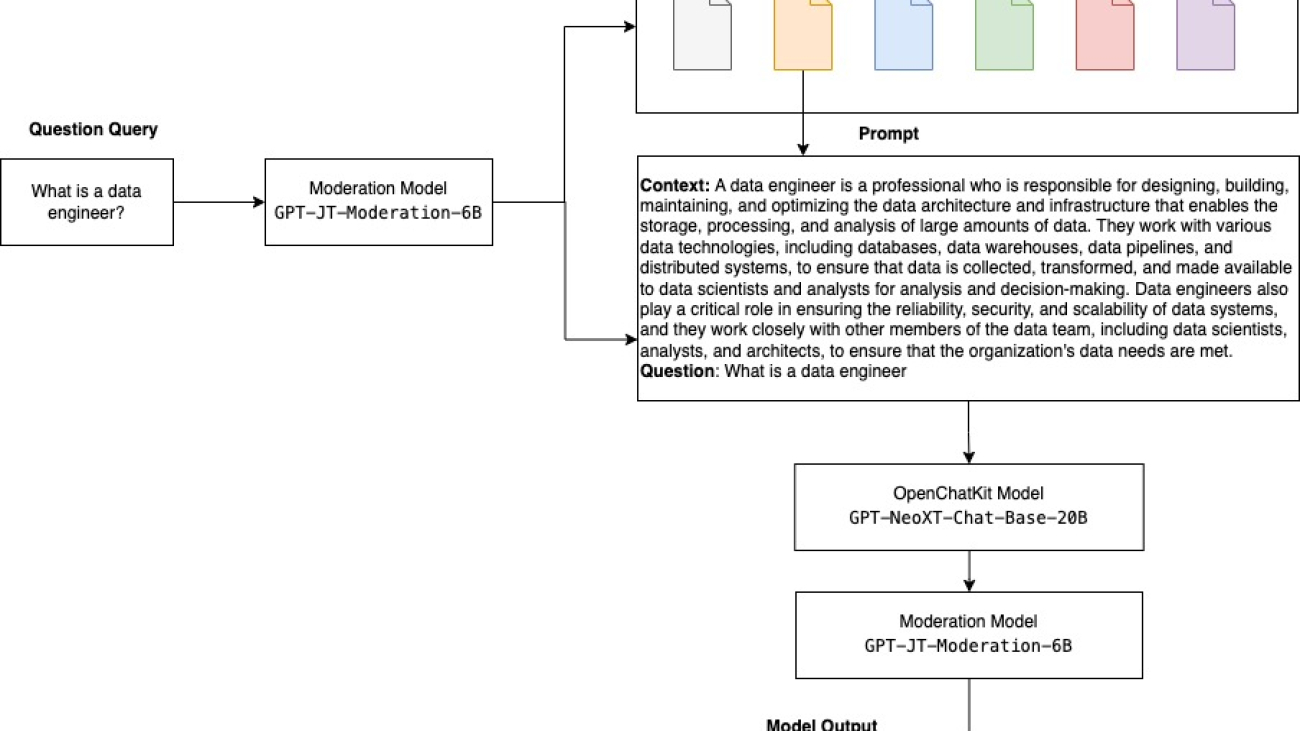
Dhawal Patel is a Principal Machine Learning Architect at AWS. He has worked with organizations ranging from large enterprises to mid-sized startups on problems related to distributed computing, and Artificial Intelligence. He focuses on Deep learning including NLP and Computer Vision domains. He helps customers achieve high performance model inference on SageMaker.

Vikram Elango is a Sr. AIML Specialist Solutions Architect at AWS, based in Virginia, US. He is currently focused on generative AI, LLMs, prompt engineering, large model inference optimization, and scaling ML across enterprises. Vikram helps financial and insurance industry customers with design and thought leadership to build and deploy machine learning applications at scale. In his spare time, he enjoys traveling, hiking, cooking, and camping with his family.

Andrew Smith is a Cloud Support Engineer in the SageMaker, Vision & Other team at AWS, based in Sydney, Australia. He supports customers using many AI/ML services on AWS with expertise in working with Amazon SageMaker. Outside of work, he enjoys spending time with friends and family as well as learning about different technologies.

Read More

GPT-J is an open-source 6-billion-parameter model released by Eleuther AI. The model is trained on the Pile and can perform various tasks in language processing. It can support a wide variety of use cases, including text classification, token classification, text generation, question and answering, entity extraction, summarization, sentiment analysis, and many more. GPT-J is a transformer model trained using Ben Wang’s Mesh Transformer JAX.

In this post, we present a guide and best practices on training large language models (LLMs) using the Amazon SageMaker distributed model parallel library to reduce training time and cost. You will learn how to train a 6-billion-parameter GPT-J model on SageMaker with ease. Finally, we share the main features of SageMaker distributed model parallelism that help with speeding up training time.

Transformer neural networks

A transformer neural network is a popular deep learning architecture to solve sequence-to-sequence tasks. It uses attention as the learning mechanism to achieve close to human-level performance. Some of the other useful properties of the architecture compared to previous generations of natural language processing (NLP) models include the ability distribute, scale, and pre-train. Transformers-based models can be applied across different use cases when dealing with text data, such as search, chatbots, and many more. Transformers use the concept of pre-training to gain intelligence from large datasets. Pre-trained transformers can be used as is or fine-tuned on your datasets, which can be much smaller and specific to your business.

Hugging Face on SageMaker

Hugging Face is a company developing some of the most popular open-source libraries providing state-of-the-art NLP technology based on transformers architectures. The Hugging Face transformers, tokenizers, and datasets libraries provide APIs and tools to download and predict using pre-trained models in multiple languages. SageMaker enables you to train, fine-tune, and run inference using Hugging Face models directly from its Hugging Face Model Hub using the Hugging Face estimator in the SageMaker SDK. The integration makes it easier to customize Hugging Face models on domain-specific use cases. Behind the scenes, the SageMaker SDK uses AWS Deep Learning Containers (DLCs), which are a set of prebuilt Docker images for training and serving models offered by SageMaker. The DLCs are developed through a collaboration between AWS and Hugging Face. The integration also offers integration between the Hugging Face transformers SDK and SageMaker distributed training libraries, enabling you to scale your training jobs on a cluster of GPUs.

Overview of the SageMaker distributed model parallel library

Model parallelism is a distributed training strategy that partitions the deep learning model over numerous devices, within or across instances. Deep learning (DL) models with more layers and parameters perform better in complex tasks like computer vision and NLP. However, the maximum model size that can be stored in the memory of a single GPU is limited. GPU memory constraints can be bottlenecks while training DL models in the following ways:

• They limit the size of the model that can be trained because a model’s memory footprint scales proportionately to the number of parameters
• They reduce GPU utilization and training efficiency by limiting the per-GPU batch size during training

SageMaker includes the distributed model parallel library to help distribute and train DL models effectively across many compute nodes, overcoming the restrictions associated with training a model on a single GPU. Furthermore, the library allows you to obtain the most optimal distributed training utilizing EFA-supported devices, which improves inter-node communication performance with low latency, high throughput, and OS bypass.

Because large models such as GPT-J, with billions of parameters, have a GPU memory footprint that exceeds a single chip, it becomes essential to partition them across multiple GPUs. The SageMaker model parallel (SMP) library enables automatic partitioning of models across multiple GPUs. With SageMaker model parallelism, SageMaker runs an initial profiling job on your behalf to analyze the compute and memory requirements of the model. This information is then used to decide how the model is partitioned across GPUs, in order to maximize an objective, such as maximizing speed or minimizing memory footprint.

It also supports optional pipeline run scheduling in order to maximize the overall utilization of available GPUs. The propagation of activations during forward pass and gradients during backward pass requires sequential computation, which limits the amount of GPU utilization. SageMaker overcomes the sequential computation constraint utilizing the pipeline run schedule by splitting mini-batches into micro-batches to be processed in parallel on different GPUs. SageMaker model parallelism supports two modes of pipeline runs:

• Simple pipeline – This mode finishes the forward pass for each micro-batch before starting the backward pass.
• Interleaved pipeline – In this mode, the backward run of the micro-batches is prioritized whenever possible. This allows for quicker release of the memory used for activations, thereby using memory more efficiently.

Tensor parallelism

Individual layers, ornn.Modules, are divided across devices using tensor parallelism so they can run concurrently. The simplest example of how the library divides a model with four layers to achieve two-way tensor parallelism ("tensor_parallel_degree": 2) is shown in the following figure. Each model replica’s layers are bisected (divided in half) and distributed between two GPUs. The degree of data parallelism is eight in this example because the model parallel configuration additionally includes "pipeline_parallel_degree": 1 and "ddp": True. The library manages communication among the replicas of the tensor-distributed model.

The benefit of this feature is that you may choose which layers or which subset of layers you want to apply tensor parallelism to. To dive deep into tensor parallelism and other memory-saving features for PyTorch, and to learn how to set up a combination of pipeline and tensor parallelism, see Extended Features of the SageMaker Model Parallel Library for PyTorch.

SageMaker sharded data parallelism

Sharded data parallelism is a memory-saving distributed training technique that splits the training state of a model (model parameters, gradients, and optimizer states) across GPUs in a data parallel group.

When scaling up your training job to a large GPU cluster, you can reduce the per-GPU memory footprint of the model by sharding the training state over multiple GPUs. This returns two benefits: you can fit larger models, which would otherwise run out of memory with standard data parallelism, or you can increase the batch size using the freed-up GPU memory.

The standard data parallelism technique replicates the training states across the GPUs in the data parallel group and performs gradient aggregation based on the AllReduce operation. In effect, sharded data parallelism introduces a trade-off between the communication overhead and GPU memory efficiency. Using sharded data parallelism increases the communication cost, but the memory footprint per GPU (excluding the memory usage due to activations) is divided by the sharded data parallelism degree, therefore larger models can fit in a GPU cluster.

SageMaker implements sharded data parallelism through the MiCS implementation. For more information, see Near-linear scaling of gigantic-model training on AWS.

Refer to Sharded Data Parallelism for further details on how to apply sharded data parallelism to your training jobs.

Use the SageMaker model parallel library

The SageMaker model parallel library comes with the SageMaker Python SDK. You need to install the SageMaker Python SDK to use the library, and it’s already installed on SageMaker notebook kernels. To make your PyTorch training script utilize the capabilities of the SMP library, you need to make the following changes:

1. Strat by importing and initializing the smp library using the smp.init()call.
2. Once it’s initialized, you can wrap your model with the smp.DistributedModel wrapper and use the returned DistributedModel object instead of the user model.
3. For your optimizer state, use the smp.DistributedOptimizer wrapper around your model optimizer, enabling smp to save and load the optimizer state. The forward and backward pass logic can be abstracted as a separate function and add a smp.step decorator to the function. Essentially, the forward pass and back-propagation needs to be run inside the function with the smp.step decorator placed over it. This allows smp to split the tensor input to the function into a number of microbatches specified while launching the training job.
4. Next, we can move the input tensors to the GPU used by the current process using the torch.cuda.set_device API followed by the .to() API call.
5. Finally, for back-propagation, we replace torch.Tensor.backward and torch.autograd.backward.

See the following code:

@smp.step
def train_step(model, data, target):
    output = model(data)
    loss = F.nll_loss(output, target, reduction="mean")
    model.backward(Loss)
    
    return output, loss

with smp.tensor_parallelism():
    model = AutoModelForCausalLM.from_config(model_config)
    
model = smp.DistributedModel (model)
optimizer = smp. DistributedOptimizer(optimizer)

The SageMaker model parallel library’s tensor parallelism offers out-of-the-box support for the following Hugging Face Transformer models:

• GPT-2, BERT, and RoBERTa (available in the SMP library v1.7.0 and later)
• GPT-J (available in the SMP library v1.8.0 and later)
• GPT-Neo (available in the SMP library v1.10.0 and later)

Best practices for performance tuning with the SMP library

When training large models, consider the following steps so that your model fits in GPU memory with a reasonable batch size:

• It’s recommended to use instances with higher GPU memory and high bandwidth interconnect for performance, such as p4d and p4de instances.
• Optimizer state sharding can be enabled in most cases, and will be helpful when you have more than one copy of the model (data parallelism enabled). You can turn on optimizer state sharding by setting "shard_optimizer_state": True in the modelparallel configuration.
• Use activation checkpointing, a technique to reduce memory usage by clearing activations of certain layers and recomputing them during a backward pass of selected modules in the model.
• Use activation offloading, an additional feature that can further reduce memory usage. To use activation offloading, set "offload_activations": True in the modelparallel configuration. Use when activation checkpointing and pipeline parallelism are turned on and the number of microbatches is greater than one.
• Enable tensor parallelism and increase parallelism degrees where the degree is a power of 2. Typically for performance reasons, tensor parallelism is restricted to within a node.

We have run many experiments to optimize training and tuning GPT-J on SageMaker with the SMP library. We have managed to reduce GPT-J training time for an epoch on SageMaker from 58 minutes to less than 10 minutes—six times faster training time per epoch. It took initialization, model and dataset download from Amazon Simple Storage Service (Amazon S3) less than a minute, tracing and auto partitioning with GPU as the tracing device less than 1 minute, and training an epoch 8 minutes using tensor parallelism on one ml.p4d.24xlarge instance, FP16 precision, and a SageMaker Hugging Face estimator.

To reduce training time as a best practice, when training GPT-J on SageMaker, we recommend the following:

• Store your pretrained model on Amazon S3
• Use FP16 precision
• Use GPU as a tracing device
• Use auto-partitioning, activation checkpointing, and optimizer state sharding:
  • auto_partition: True
  • shard_optimizer_state: True
• Use tensor parallelism
• Use a SageMaker training instance with multiple GPUs such as ml.p3.16xlarge, ml.p3dn.24xlarge, ml.g5.48xlarge, ml.p4d.24xlarge, or ml.p4de.24xlarge.

GPT-J model training and tuning on SageMaker with the SMP library

A working step-by-step code sample is available on the Amazon SageMaker Examples public repository. Navigate to the training/distributed_training/pytorch/model_parallel/gpt-j folder. Select the gpt-j folder and open the train_gptj_smp_tensor_parallel_notebook.jpynb Jupyter notebook for the tensor parallelism example and train_gptj_smp_notebook.ipynb for the pipeline parallelism example. You can find a code walkthrough in our Generative AI on Amazon SageMaker workshop.

This notebook walks you through how to use the tensor parallelism features provided by the SageMaker model parallelism library. You’ll learn how to run FP16 training of the GPT-J model with tensor parallelism and pipeline parallelism on the GLUE sst2 dataset.

Summary

The SageMaker model parallel library offers several functionalities. You can reduce cost and speed up training LLMs on SageMaker. You can also learn and run sample codes for BERT, GPT-2, and GPT-J on the Amazon SageMaker Examples public repository. To learn more about AWS best practices for training LLMS using the SMP library, refer to the following resources:

• SageMaker Distributed Model Parallelism Best Practices
• Training large language models on Amazon SageMaker: Best practices

To learn how one of our customers achieved low-latency GPT-J inference on SageMaker, refer to How Mantium achieves low-latency GPT-J inference with DeepSpeed on Amazon SageMaker.

If you’re looking to accelerate time-to-market of your LLMs and reduce your costs, SageMaker can help. Let us know what you build!

About the Authors

Zmnako Awrahman, PhD, is a Practice Manager, ML SME, and Machine Learning Technical Field Community (TFC) member at Global Competency Center, Amazon Web Services. He helps customers leverage the power of the cloud to extract value from their data with data analytics and machine learning.

Roop Bains is a Senior Machine Learning Solutions Architect at AWS. He is passionate about helping customers innovate and achieve their business objectives using artificial intelligence and machine learning. He helps customers train, optimize, and deploy deep learning models.

Anastasia Pachni Tsitiridou is a Solutions Architect at AWS. Anastasia lives in Amsterdam and supports software businesses across the Benelux region in their cloud journey. Prior to joining AWS, she studied electrical and computer engineering with a specialization in computer vision. What she enjoys most nowadays is working with very large language models.

Dhawal Patel is a Principal Machine Learning Architect at AWS. He has worked with organizations ranging from large enterprises to mid-sized startups on problems related to distributed computing and artificial intelligence. He focuses on deep learning, including NLP and computer vision domains. He helps customers achieve high-performance model inference on SageMaker.

Wioletta Stobieniecka is a Data Scientist at AWS Professional Services. Throughout her professional career, she has delivered multiple analytics-driven projects for different industries such as banking, insurance, telco, and the public sector. Her knowledge of advanced statistical methods and machine learning is well combined with a business acumen. She brings recent AI advancements to create value for customers.

Rahul Huilgol is a Senior Software Development Engineer in Distributed Deep Learning at Amazon Web Services.

Read More

ONNX (Open Neural Network Exchange) is an open-source standard for representing deep learning models widely supported by many providers. ONNX provides tools for optimizing and quantizing models to reduce the memory and compute needed to run machine learning (ML) models. One of the biggest benefits of ONNX is that it provides a standardized format for representing and exchanging ML models between different frameworks and tools. This allows developers to train their models in one framework and deploy them in another without the need for extensive model conversion or retraining. For these reasons, ONNX has gained significant importance in the ML community.

In this post, we showcase how to deploy ONNX-based models for multi-model endpoints (MMEs) that use GPUs. This is a continuation of the post Run multiple deep learning models on GPU with Amazon SageMaker multi-model endpoints, where we showed how to deploy PyTorch and TensorRT versions of ResNet50 models on Nvidia’s Triton Inference server. In this post, we use the same ResNet50 model in ONNX format along with an additional natural language processing (NLP) example model in ONNX format to show how it can be deployed on Triton. Furthermore, we benchmark the ResNet50 model and see the performance benefits that ONNX provides when compared to PyTorch and TensorRT versions of the same model, using the same input.

ONNX Runtime

ONNX Runtime is a runtime engine for ML inference designed to optimize the performance of models across multiple hardware platforms, including CPUs and GPUs. It allows the use of ML frameworks like PyTorch and TensorFlow. It facilitates performance tuning to run models cost-efficiently on the target hardware and has support for features like quantization and hardware acceleration, making it one of the ideal choices for deploying efficient, high-performance ML applications. For examples of how ONNX models can be optimized for Nvidia GPUs with TensorRT, refer to TensorRT Optimization (ORT-TRT) and ONNX Runtime with TensorRT optimization.

The Amazon SageMaker Triton container flow is depicted in the following diagram.

Users can send an HTTPS request with the input payload for real-time inference behind a SageMaker endpoint. The user can specify a TargetModel header that contains the name of the model that the request in question is destined to invoke. Internally, the SageMaker Triton container implements an HTTP server with the same contracts as mentioned in How Containers Serve Requests. It has support for dynamic batching and supports all the backends that Triton provides. Based on the configuration, the ONNX runtime is invoked and the request is processed on CPU or GPU as predefined in the model configuration provided by the user.

Solution overview

To use the ONNX backend, complete the following steps:

1. Compile the model to ONNX format.
2. Configure the model.
3. Create the SageMaker endpoint.

Prerequisites

Ensure that you have access to an AWS account with sufficient AWS Identity and Access Management IAM permissions to create a notebook, access an Amazon Simple Storage Service (Amazon S3) bucket, and deploy models to SageMaker endpoints. See Create execution role for more information.

Compile the model to ONNX format

The transformers library provides for convenient method to compile the PyTorch model to ONNX format. The following code achieves the transformations for the NLP model:

onnx_inputs, onnx_outputs = transformers.onnx.export(
    preprocessor=tokenizer,
    model=model,
    config=onnx_config,
    opset=12,
    output=save_path
 )

Exporting models (either PyTorch or TensorFlow) is easily achieved through the conversion tool provided as part of the Hugging Face transformers repository.

The following is what happens under the hood:

1. Allocate the model from transformers (PyTorch or TensorFlow).
2. Forward dummy inputs through the model. This way, ONNX can record the set of operations run.
3. The transformers inherently take care of dynamic axes when exporting the model.
4. Save the graph along with the network parameters.

A similar mechanism is followed for the computer vision use case from the torchvision model zoo:

torch.onnx.export(
        resnet50,
        dummy_input,
        args.save,
        export_params=True,
        opset_version=11,
        do_constant_folding=True,
        input_names=["input"],
        output_names=["output"],
        dynamic_axes={"input": {0: "batch_size"}, "output": {0: "batch_size"}},
    )

Configure the model

In this section, we configure the computer vision and NLP model. We show how to create a ResNet50 and RoBERTA large model that has been pre-trained for deployment on a SageMaker MME by utilizing Triton Inference Server model configurations. The ResNet50 notebook is available on GitHub. The RoBERTA notebook is also available on GitHub. For ResNet50, we use the Docker approach to create an environment that already has all the dependencies required to build our ONNX model and generate the model artifacts needed for this exercise. This approach makes it much easier to share dependencies and create the exact environment that is needed to accomplish this task.

The first step is to create the ONNX model package per the directory structure specified in ONNX Models. Our aim is to use the minimal model repository for a ONNX model contained in a single file as follows:

<model-repository-path> / 
    Model_name
    ├── 1
    │   └── model.onnx
    └── config.pbtxt

Next, we create the model configuration file that describes the inputs, outputs, and backend configurations for the Triton Server to pick up and invoke the appropriate kernels for ONNX. This file is known as config.pbtxt and is shown in the following code for the RoBERTA use case. Note that the BATCH dimension is omitted from the config.pbtxt. However, when sending the data to the model, we include the batch dimension. The following code also shows how you can add this feature with model configuration files to set dynamic batching with a preferred batch size of 5 for the actual inference. With the current settings, the model instance is invoked instantly when the preferred batch size of 5 is met or the delay time of 100 microseconds has elapsed since the first request reached the dynamic batcher.

name: "nlp-onnx"
platform: "onnxruntime_onnx"
backend: "onnxruntime" 
max_batch_size: 32

  input {
    name: "input_ids"
    data_type: TYPE_INT64
    dims: [512]
  }
  input {
    name: "attention_mask"
    data_type: TYPE_INT64
    dims: [512]
  }

  output {
    name: "last_hidden_state"
    data_type: TYPE_FP32
    dims: [-1, 768]
  }
  output {
    name: "1550"
    data_type: TYPE_FP32
    dims: [768]
  }
instance_group {
  count: 1
  kind: KIND_GPU
}
dynamic_batching {
    max_queue_delay_microseconds: 100
    preferred_batch_size:5
}

The following is the similar configuration file for the computer vision use case:

name: "resenet_onnx"
platform: "onnxruntime_onnx"
max_batch_size : 128
input [
  {
    name: "input"
    data_type: TYPE_FP32
    format: FORMAT_NCHW
    dims: [ 3, 224, 224 ]
  }
]
output [
  {
    name: "output"
    data_type: TYPE_FP32
    dims: [ 1000 ]
  }
]

Create the SageMaker endpoint

We use the Boto3 APIs to create the SageMaker endpoint. For this post, we show the steps for the RoBERTA notebook, but these are common steps and will be the same for the ResNet50 model as well.

Create a SageMaker model

We now create a SageMaker model. We use the Amazon Elastic Container Registry (Amazon ECR) image and the model artifact from the previous step to create the SageMaker model.

Create the container

To create the container, we pull the appropriate image from Amazon ECR for Triton Server. SageMaker allows us to customize and inject various environment variables. Some of the key features are the ability to set the BATCH_SIZE; we can set this per model in the config.pbtxt file, or we can define a default value here. For models that can benefit from larger shared memory size, we can set those values under SHM variables. To enable logging, set the log verbose level to true. We use the following code to create the model to use in our endpoint:

mme_triton_image_uri = (
    f"{account_id_map[region]}.dkr.ecr.{region}.{base}" + "/sagemaker-tritonserver:22.12-py3"
)
container = {
    "Image": mme_triton_image_uri,
    "ModelDataUrl": mme_path,
    "Mode": "MultiModel",
    "Environment": {
        "SAGEMAKER_TRITON_SHM_DEFAULT_BYTE_SIZE": "16777216000", # "16777216", #"16777216000",
        "SAGEMAKER_TRITON_SHM_GROWTH_BYTE_SIZE": "10485760",
    },
}
from sagemaker.utils import name_from_base
model_name = name_from_base(f"flan-xxl-fastertransformer")
print(model_name)
create_model_response = sm_client.create_model(
    ModelName=model_name,
    ExecutionRoleArn=role,
    PrimaryContainer={
        "Image": inference_image_uri, 
        "ModelDataUrl": s3_code_artifact
    },
)
model_arn = create_model_response["ModelArn"]
print(f"Created Model: {model_arn}")

Create a SageMaker endpoint

You can use any instances with multiple GPUs for testing. In this post, we use a g4dn.4xlarge instance. We don’t set the VolumeSizeInGB parameters because this instance comes with local instance storage. The VolumeSizeInGB parameter is applicable to GPU instances supporting the Amazon Elastic Block Store (Amazon EBS) volume attachment. We can leave the model download timeout and container startup health check at the default values. For more details, refer to CreateEndpointConfig.

endpoint_config_response = sm_client.create_endpoint_config(
EndpointConfigName=endpoint_config_name,
    ProductionVariants=[{
            "VariantName": "AllTraffic",
            "ModelName": model_name,
            "InstanceType": "ml.g4dn.4xlarge",
            "InitialInstanceCount": 1,
            #"VolumeSizeInGB" : 200,
            #"ModelDataDownloadTimeoutInSeconds": 600,
            #"ContainerStartupHealthCheckTimeoutInSeconds": 600,
        },
    ],)'

Lastly, we create a SageMaker endpoint:

create_endpoint_response = sm_client.create_endpoint(
EndpointName=f"{endpoint_name}", EndpointConfigName=endpoint_config_name)

Invoke the model endpoint

This is a generative model, so we pass in the input_ids and attention_mask to the model as part of the payload. The following code shows how to create the tensors:

tokenizer("This is a sample", padding="max_length", max_length=max_seq_len)

We now create the appropriate payload by ensuring the data type matches what we configured in the config.pbtxt. This also give us the tensors with the batch dimension included, which is what Triton expects. We use the JSON format to invoke the model. Triton also provides a native binary invocation method for the model.

response = runtime_sm_client.invoke_endpoint(
    EndpointName=endpoint_name,
    ContentType="application/octet-stream",
    Body=json.dumps(payload),
    TargetModel=f"{tar_file_name}",
    # TargetModel=f"roberta-large-v0.tar.gz",
)

Note the TargetModel parameter in the preceding code. We send the name of the model to be invoked as a request header because this is a multi-model endpoint, therefore we can invoke multiple models at runtime on an already deployed inference endpoint by changing this parameter. This shows the power of multi-model endpoints!

To output the response, we can use the following code:

import numpy as np

resp_bin = response["Body"].read().decode("utf8")
# -- keys are -- "outputs":[{"name":"1550","datatype":"FP32","shape":[1,768],"data": [0.0013,0,3433...]}]
for data in json.loads(resp_bin)["outputs"]:
    shape_1 = list(data["shape"])
    dat_1 = np.array(data["data"])
    dat_1.resize(shape_1)
    print(f"Data Outputs recieved back :Shape:{dat_1.shape}")

ONNX for performance tuning

The ONNX backend uses C++ arena memory allocation. Arena allocation is a C++-only feature that helps you optimize your memory usage and improve performance. Memory allocation and deallocation constitutes a significant fraction of CPU time spent in protocol buffers code. By default, new object creation performs heap allocations for each object, each of its sub-objects, and several field types, such as strings. These allocations occur in bulk when parsing a message and when building new messages in memory, and associated deallocations happen when messages and their sub-object trees are freed.

Arena-based allocation has been designed to reduce this performance cost. With arena allocation, new objects are allocated out of a large piece of pre-allocated memory called the arena. Objects can all be freed at once by discarding the entire arena, ideally without running destructors of any contained object (though an arena can still maintain a destructor list when required). This makes object allocation faster by reducing it to a simple pointer increment, and makes deallocation almost free. Arena allocation also provides greater cache efficiency: when messages are parsed, they are more likely to be allocated in continuous memory, which makes traversing messages more likely to hit hot cache lines. The downside of arena-based allocation is the C++ heap memory will be over-allocated and stay allocated even after the objects are deallocated. This might lead to out of memory or high CPU memory usage. To achieve the best of both worlds, we use the following configurations provided by Triton and ONNX:

• arena_extend_strategy – This parameter refers to the strategy used to grow the memory arena with regards to the size of the model. We recommend setting the value to 1 (= kSameAsRequested), which is not a default value. The reasoning is as follows: the drawback of the default arena extend strategy (kNextPowerOfTwo) is that it might allocate more memory than needed, which could be a waste. As the name suggests, kNextPowerOfTwo (the default) extends the arena by a power of 2, whereas kSameAsRequested extends by a size that is the same as the allocation request each time. kSameAsRequested is suited for advanced configurations where you know the expected memory usage in advance. In our testing, because we know the size of models is a constant value, we can safely choose kSameAsRequested.
• gpu_mem_limit – We set the value to the CUDA memory limit. To use all possible memory, pass in the maximum size_t. It defaults to SIZE_MAX if nothing is specified. We recommend keeping it as default.
• enable_cpu_mem_arena – This enables the memory arena on CPU. The arena may pre-allocate memory for future usage. Set this option to false if you don’t want it. The default is True. If you disable the arena, heap memory allocation will take time, so inference latency will increase. In our testing, we left it as default.
• enable_mem_pattern – This parameter refers to the internal memory allocation strategy based on input shapes. If the shapes are constant, we can enable this parameter to generate a memory pattern for the future and save some allocation time, making it faster. Use 1 to enable the memory pattern and 0 to disable. It’s recommended to set this to 1 when the input features are expected to be the same. The default value is 1.
• do_copy_in_default_stream – In the context of the CUDA execution provider in ONNX, a compute stream is a sequence of CUDA operations that are run asynchronously on the GPU. The ONNX runtime schedules operations in different streams based on their dependencies, which helps minimize the idle time of the GPU and achieve better performance. We recommend using the default setting of 1 for using the same stream for copying and compute; however, you can use 0 for using separate streams for copying and compute, which might result in the device pipelining the two activities. In our testing of the ResNet50 model, we used both 0 and 1 but couldn’t find any appreciable difference between the two in terms of performance and memory consumption of the GPU device.
• Graph optimization – The ONNX backend for Triton supports several parameters that help fine-tune the model size as well as runtime performance of the deployed model. When the model is converted to the ONNX representation (the first box in the following diagram at the IR stage), the ONNX runtime provides graph optimizations at three levels: basic, extended, and layout optimizations. You can activate all levels of graph optimizations by adding the following parameters in the model configuration file:

  optimization {
    graph : {
      level : 1
  }}

• cudnn_conv_algo_search – Because we’re using CUDA-based Nvidia GPUs in our testing, for our computer vision use case with the ResNet50 model, we can use the CUDA execution provider-based optimization at the fourth layer in the following diagram with the cudnn_conv_algo_search parameter. The default option is exhaustive (0), but when we changed this configuration to 1 – HEURISTIC, we saw the model latency in steady state reduce to 160 milliseconds. The reason this happens is because the ONNX runtime invokes the lighter weight cudnnGetConvolutionForwardAlgorithm_v7 forward pass and therefore reduces latency with adequate performance.
• Run mode – The next step is selecting the correct execution_mode at layer 5 in the following diagram. This parameter controls whether you want to run operators in your graph sequentially or in parallel. Usually when the model has many branches, setting this option to ExecutionMode.ORT_PARALLEL (1) will give you better performance. In the scenario where your model has many branches in its graph, setting the run mode to parallel will help with better performance. The default mode is sequential, so you can enable this to suit your needs.

  parameters { key: "execution_mode" value: { string_value: "1" } }

For a deeper understanding of the opportunities for performance tuning in ONNX, refer to the following figure.

Source: https://static.linaro.org/connect/san19/presentations/san19-211.pdf

Benchmark numbers and performance tuning

By turning on the graph optimizations, cudnn_conv_algo_search, and parallel run mode parameters in our testing of the ResNet50 model, we saw the cold start time of the ONNX model graph reduce from 4.4 seconds to 1.61 seconds. An example of a complete model configuration file is provided in the ONNX configuration section of the following notebook.

The testing benchmark results are as follows:

• PyTorch – 176 milliseconds, cold start 6 seconds
• TensorRT – 174 milliseconds, cold start 4.5 seconds
• ONNX – 168 milliseconds, cold start 4.4 seconds

The following graphs visualize these metrics.

Furthermore, in our testing of computer vision use cases, consider sending the request payload in binary format using the HTTP client provided by Triton because it significantly improves model invoke latency.

Other parameters that SageMaker exposes for ONNX on Triton are as follows:

• Dynamic batching – Dynamic batching is a feature of Triton that allows inference requests to be combined by the server, so that a batch is created dynamically. Creating a batch of requests typically results in increased throughput. The dynamic batcher should be used for stateless models. The dynamically created batches are distributed to all model instances configured for the model.
• Maximum batch size – The max_batch_size property indicates the maximum batch size that the model supports for the types of batching that can be exploited by Triton. If the model’s batch dimension is the first dimension, and all inputs and outputs to the model have this batch dimension, then Triton can use its dynamic batcher or sequence batcher to automatically use batching with the model. In this case, max_batch_size should be set to a value greater than or equal to 1, which indicates the maximum batch size that Triton should use with the model.
• Default max batch size – The default-max-batch-size value is used for max_batch_size during autocomplete when no other value is found. The onnxruntime backend will set the max_batch_size of the model to this default value if autocomplete has determined the model is capable of batching requests and max_batch_size is 0 in the model configuration or max_batch_size is omitted from the model configuration. If max_batch_size is more than 1 and no scheduler is provided, the dynamic batch scheduler will be used. The default max batch size is 4.

Clean up

Ensure that you delete the model, model configuration, and model endpoint after running the notebook. The steps to do this are provided at the end of the sample notebook in the GitHub repo.

Conclusion

In this post, we dove deep into the ONNX backend that Triton Inference Server supports on SageMaker. This backend provides for GPU acceleration of your ONNX models. There are many options to consider to get the best performance for inference, such as batch sizes, data input formats, and other factors that can be tuned to meet your needs. SageMaker allows you to use this capability using single-model and multi-model endpoints. MMEs allow a better balance of performance and cost savings. To get started with MME support for GPU, see Host multiple models in one container behind one endpoint.

We invite you to try Triton Inference Server containers in SageMaker, and share your feedback and questions in the comments.

About the authors

Abhi Shivaditya is a Senior Solutions Architect at AWS, working with strategic global enterprise organizations to facilitate the adoption of AWS services in areas such as Artificial Intelligence, distributed computing, networking, and storage. His expertise lies in Deep Learning in the domains of Natural Language Processing (NLP) and Computer Vision. Abhi assists customers in deploying high-performance machine learning models efficiently within the AWS ecosystem.

James Park is a Solutions Architect at Amazon Web Services. He works with Amazon.com to design, build, and deploy technology solutions on AWS, and has a particular interest in AI and machine learning. In h is spare time he enjoys seeking out new cultures, new experiences,  and staying up to date with the latest technology trends.You can find him on LinkedIn.

Rupinder Grewal is a Sr Ai/ML Specialist Solutions Architect with AWS. He currently focuses on serving of models and MLOps on SageMaker. Prior to this role he has worked as Machine Learning Engineer building and hosting models. Outside of work he enjoys playing tennis and biking on mountain trails.

Dhawal Patel is a Principal Machine Learning Architect at AWS. He has worked with organizations ranging from large enterprises to mid-sized startups on problems related to distributed computing, and Artificial Intelligence. He focuses on Deep learning including NLP and Computer Vision domains. He helps customers achieve high performance model inference on SageMaker.

Read More

We are excited to announce the open-source release of GraphStorm 0.1, a low-code enterprise graph machine learning (ML) framework to build, train, and deploy graph ML solutions on complex enterprise-scale graphs in days instead of months. With GraphStorm, you can build solutions that directly take into account the structure of relationships or interactions between billions of entities, which are inherently embedded in most real-world data, including fraud detection scenarios, recommendations, community detection, and search/retrieval problems.

Until now, it has been notoriously hard to build, train, and deploy graph ML solutions for complex enterprise graphs that easily have billions of nodes, hundreds of billions of edges, and dozens of attributes—just think about a graph capturing Amazon.com products, product attributes, customers, and more. With GraphStorm, we release the tools that Amazon uses internally to bring large-scale graph ML solutions to production. GraphStorm doesn’t require you to be an expert in graph ML and is available under the Apache v2.0 license on GitHub. To learn more about GraphStorm, visit the GitHub repository.

In this post, we provide an introduction to GraphStorm, its architecture, and an example use case of how to use it.

Introducing GraphStorm

Graph algorithms and graph ML are emerging as state-of-the-art solutions for many important business problems like predicting transaction risks, anticipating customer preferences, detecting intrusions, optimizing supply chains, social network analysis, and traffic prediction. For example, Amazon GuardDuty, the native AWS threat detection service, uses a graph with billions of edges to improve the coverage and accuracy of its threat intelligence. This allows GuardDuty to categorize previously unseen domains as highly likely to be malicious or benign based on their association to known malicious domains. By using Graph Neural Networks (GNNs), GuardDuty is able to enhance its capability to alert customers.

However, developing, launching, and operating graph ML solutions takes months and requires graph ML expertise. As a first step, a graph ML scientist has to build a graph ML model for a given use case using a framework like the Deep Graph Library (DGL). Training such models is challenging due to the size and complexity of graphs in enterprise applications, which routinely reach billions of nodes, hundreds of billions of edges, different node and edge types, and hundreds of node and edge attributes. Enterprise graphs can require terabytes of memory storage, requiring graph ML scientists to build complex training pipelines. Finally, after a model has been trained, they have to be deployed for inference, which requires inference pipelines that are just as difficult to build as the training pipelines.

GraphStorm 0.1 is a low-code enterprise graph ML framework that allows ML practitioners to easily pick predefined graph ML models that have been proven to be effective, run distributed training on graphs with billions of nodes, and deploy the models into production. GraphStorm offers a collection of built-in graph ML models, such as Relational Graph Convolutional Networks (RGCN), Relational Graph Attention Networks (RGAT), and Heterogeneous Graph Transformer (HGT) for enterprise applications with heterogeneous graphs, which allow ML engineers with little graph ML expertise to try out different model solutions for their task and select the right one quickly. End-to-end distributed training and inference pipelines, which scale to billion-scale enterprise graphs, make it easy to train, deploy, and run inference. If you are new to GraphStorm or graph ML in general, you will benefit from the pre-defined models and pipelines. If you are an expert, you have all options to tune the training pipeline and model architecture to get the best performance. GraphStorm is built on top of the DGL, a widely popular framework for developing GNN models, and available as open-source code under the Apache v2.0 license.

“GraphStorm is designed to help customers experiment and operationalize graph ML methods for industry applications to accelerate the adoption of graph ML,” says George Karypis, Senior Principal Scientist in Amazon AI/ML research. “Since its release inside Amazon, GraphStorm has reduced the effort to build graph ML-based solutions by up to five times.”

“GraphStorm enables our team to train GNN embedding in a self-supervised manner on a graph with 288 million nodes and 2 billion edges,” Says Haining Yu, Principal Applied Scientist at Amazon Measurement, Ad Tech, and Data Science. “The pre-trained GNN embeddings show a 24% improvement on a shopper activity prediction task over a state-of-the-art BERT- based baseline; it also exceeds benchmark performance in other ads applications.”

“Before GraphStorm, customers could only scale vertically to handle graphs of 500 million edges,” says Brad Bebee, GM for Amazon Neptune and Amazon Timestream. “GraphStorm enables customers to scale GNN model training on massive Amazon Neptune graphs with tens of billions of edges.”

GraphStorm technical architecture

The following figure shows the technical architecture of GraphStorm.

GraphStorm is built on top of PyTorch and can run on a single GPU, multiple GPUs, and multiple GPU machines. It consists of three layers (marked in the yellow boxes in the preceding figure):

• Bottom layer (Dist GraphEngine) – The bottom layer provides the basic components to enable distributed graph ML, including distributed graphs, distributed tensors, distributed embeddings, and distributed samplers. GraphStorm provides efficient implementations of these components to scale graph ML training to billion-node graphs.
• Middle layer (GS training/inference pipeline) – The middle layer provides trainers, evaluators, and predictors to simplify model training and inference for both built-in models and your custom models. Basically, by using the API of this layer, you can focus on the model development without worrying about how to scale the model training.
• Top layer (GS general model zoo) – The top layer is a model zoo with popular GNN and non-GNN models for different graph types. As of this writing, it provides RGCN, RGAT, and HGT for heterogeneous graphs and BERTGNN for textual graphs. In the future, we will add support for temporal graph models such as TGAT for temporal graphs as well as TransE and DistMult for knowledge graphs.

How to use GraphStorm

After installing GraphStorm, you only need three steps to build and train GML models for your application.

First, you preprocess your data (potentially including your custom feature engineering) and transform it into a table format required by GraphStorm. For each node type, you define a table that lists all nodes of that type and their features, providing a unique ID for each node. For each edge type, you similarly define a table in which each row contains the source and destination node IDs for an edge of that type (for more information, see Use Your Own Data Tutorial). In addition, you provide a JSON file that describes the overall graph structure.

Second, via the command line interface (CLI), you use GraphStorm’s built-in construct_graph component for some GraphStorm-specific data processing, which enables efficient distributed training and inference.

Third, you configure the model and training in a YAML file (example) and, again using the CLI, invoke one of the five built-in components (gs_node_classification, gs_node_regression, gs_edge_classification, gs_edge_regression, gs_link_prediction) as training pipelines to train the model. This step results in the trained model artifacts. To do inference, you need to repeat the first two steps to transform the inference data into a graph using the same GraphStorm component (construct_graph) as before.

Finally, you can invoke one of the five built-in components, the same that was used for model training, as an inference pipeline to generate embeddings or prediction results.

The overall flow is also depicted in the following figure.

In the following section, we provide an example use case.

Make predictions on raw OAG data

For this post, we demonstrate how easily GraphStorm can enable graph ML training and inference on a large raw dataset. The Open Academic Graph (OAG) contains five entities (papers, authors, venues, affiliations, and field of study). The raw dataset is stored in JSON files with over 500 GB.

Our task is to build a model to predict the field of study of a paper. To predict the field of study, you can formulate it as a multi-label classification task, but it’s difficult to use one-hot encoding to store the labels because there are hundreds of thousands of fields. Therefore, you should create field of study nodes and formulate this problem as a link prediction task, predicting which field of study nodes a paper node should connect to.

To model this dataset with a graph method, the first step is to process the dataset and extract entities and edges. You can extract five types of edges from the JSON files to define a graph, shown in the following figure. You can use the Jupyter notebook in the GraphStorm example code to process the dataset and generate five entity tables for each entity type and five edge tables for each edge type. The Jupyter notebook also generates BERT embeddings on the entities with text data, such as papers.

After defining the entities and edges between the entities, you can create mag_bert.json, which defines the graph schema, and invoke the built-in graph construction pipeline construct_graph in GraphStorm to build the graph (see the following code). Even though the GraphStorm graph construction pipeline runs in a single machine, it supports multi-processing to process nodes and edge features in parallel (--num_processes) and can store entity and edge features on external memory (--ext-mem-workspace) to scale to large datasets.

python3 -m graphstorm.gconstruct.construct_graph 
         --num-processes 16 
         --output-dir /data/oagv2.1/mag_bert_constructed 
         --graph-name mag --num-partitions 4 
         --skip-nonexist-edges 
         --ext-mem-workspace /mnt/raid0/tmp_oag 
         --ext-mem-feat-size 16 --conf-file mag_bert.json

To process such a large graph, you need a large-memory CPU instance to construct the graph. You can use an Amazon Elastic Compute Cloud (Amazon EC2) r6id.32xlarge instance (128 vCPU and 1 TB RAM) or r6a.48xlarge instances (192 vCPU and 1.5 TB RAM) to construct the OAG graph.

After constructing a graph, you can use gs_link_prediction to train a link prediction model on four g5.48xlarge instances. When using the built-in models, you only invoke one command line to launch the distributed training job. See the following code:

python3 -m graphstorm.run.gs_link_prediction 
        --num-trainers 8 
        --part-config /data/oagv2.1/mag_bert_constructed/mag.json 
        --ip-config ip_list.txt 
        --cf ml_lp.yaml 
        --num-epochs 1 
        --save-model-path /data/mag_lp_model

After the model training, the model artifact is saved in the folder /data/mag_lp_model.

Now you can run link prediction inference to generate GNN embeddings and evaluate the model performance. GraphStorm provides multiple built-in evaluation metrics to evaluate model performance. For link prediction problems, for example, GraphStorm automatically outputs the metric mean reciprocal rank (MRR). MRR is a valuable metric for evaluating graph link prediction models because it assesses how high the actual links are ranked among the predicted links. This captures the quality of predictions, making sure our model correctly prioritizes true connections, which is our objective here.

You can run inference with one command line, as shown in the following code. In this case, the model reaches an MRR of 0.31 on the test set of the constructed graph.

python3 -m graphstorm.run.gs_link_prediction 
        --inference --num_trainers 8 
        --part-config /data/oagv2.1/mag_bert_constructed/mag.json 
        --ip-config ip_list.txt 
        --cf ml_lp.yaml 
        --num-epochs 3 
        --save-embed-path /data/mag_lp_model/emb 
        --restore-model-path /data/mag_lp_model/epoch-0/

Note that the inference pipeline generates embeddings from the link prediction model. To solve the problem of finding the field of study for any given paper, simply perform a k-nearest neighbor search on the embeddings.

Conclusion

GraphStorm is a new graph ML framework that makes it easy to build, train, and deploy graph ML models on industry graphs. It addresses some key challenges in graph ML, including scalability and usability. It provides built-in components to process billion-scale graphs from raw input data to model training and model inference and has enabled multiple Amazon teams to train state-of-the-art graph ML models in various applications. Check out our GitHub repository for more information.

About the Authors

Da Zheng is a senior applied scientist at AWS AI/ML research leading a graph machine learning team to develop techniques and frameworks to put graph machine learning in production. Da got his PhD in computer science from the Johns Hopkins University.

Florian Saupe is a Principal Technical Product Manager at AWS AI/ML research supporting advanced science teams like the graph machine learning group and improving products like Amazon DataZone with ML capabilities. Before joining AWS, Florian lead technical product management for automated driving at Bosch, was a strategy consultant at McKinsey & Company, and worked as a control systems/robotics scientist – a field in which he holds a phd.

Read More