Posts in category: Amazon AWS

In 2021, we launched AWS Support Proactive Services as part of the AWS Enterprise Support plan. Since its introduction, we’ve helped hundreds of customers optimize their workloads, set guardrails, and improve the visibility of their machine learning (ML) workloads’ cost and usage.

In this series of posts, we share lessons learned about optimizing costs in Amazon SageMaker. In this post, we focus on SageMaker training jobs.

SageMaker training jobs

SageMaker training jobs are asynchronous batch processes with built-in features for ML model training and optimization.

With SageMaker training jobs, you can bring your own algorithm or choose from more than 25 built-in algorithms. SageMaker supports various data sources and access patterns, distributed training including heterogenous clusters, as well as experiment management features and automatic model tuning.

The cost of a training job is based on the resources you use (instances and storage) for the duration (in seconds) that those instances are running. This includes the time training takes place and, if you’re using the warm pool feature, the keep alive period you configure. In Part 1, we showed how to get started using AWS Cost Explorer to identify cost optimization opportunities in SageMaker. You can filter training costs by applying a filter on the usage type. The names of these usage types are as follows:

• REGION-Train:instanceType (for example, USE1-Train:ml.m5.large)
• REGION-Train:VolumeUsage.gp2 (for example, USE1-Train:VolumeUsage.gp2)

To view a breakdown of your training costs in Cost Explorer, you can enter train: as a prefix for Usage type. If you filter only for hours used (see the following screenshot), Cost Explorer will generate two graphs: Cost and Usage. This view will help you prioritize your optimization opportunities and identify which instances are long-running and costly.

Before optimizing an existing training job, we recommend following the best practices covered in Optimizing costs for machine learning with Amazon SageMaker: test your code locally and use local mode for testing, use pre-trained models where possible, and consider managed spot training (which can optimize cost up to 90% over On-Demand instances).

When an On-Demand job is launched, it goes through five phases: Starting, Downloading, Training, Uploading, and Completed. You can see those phases and descriptions on the training job’s page on the SageMaker console.

From a pricing perspective, you are charged for Downloading, Training, and Uploading phases.

Reviewing these phases is a first step in diagnosing where to optimize your training costs. In this post, we discuss the Downloading and Training phases.

Downloading phase

In the preceding example, the Downloading phase took less than a minute. However, if data downloading is a big factor of your training cost, you should consider the data source you are using and access methods. SageMaker training jobs support three data sources natively: Amazon Elastic File System (Amazon EFS), Amazon Simple Storage Service (Amazon S3), and Amazon FSx for Lustre. For Amazon S3, SageMaker offers three managed ways that your algorithm can access the training: File mode (where data is downloaded to the instance block storage), Pipe mode (data is streamed to the instance, thereby eliminating the duration of the Downloading phase) and Fast File mode (combines the ease of use of the existing File mode with the performance of Pipe mode). For detailed guidance on choosing the right data source and access methods, refer to Choose the best data source for your Amazon SageMaker training job.

When using managed spot training, any repeated Downloading phases that occurred due to interruption are not charged (so you’re only charged for the duration of the data download one time).

It’s important to note that although SageMaker training jobs support the data sources we mentioned, they are not mandatory. In your training code, you can implement any method for downloading the training data from any source (provided that the training instance can access it). There are additional ways to speed up download time, such as using the Boto3 API with multiprocessing to download files concurrently, or using third-party libraries such as WebDataset or s5cmd for faster download from Amazon S3. For more information, refer to Parallelizing S3 Workloads with s5cmd.

Training phase

Optimizing the Training phase cost consists of optimizing two vectors: choosing the right infrastructure (instance family and size), and optimizing the training itself. We can roughly divide training instances into two categories: accelerated GPU-based, mostly for deep-learning models, and CPU-based for common ML frameworks. For guidance on selecting the right instance family for training, refer to Ensure efficient compute resources on Amazon SageMaker. If your training requires GPUs instances, we recommend referring to the video How to select Amazon EC2 GPU instances for deep learning.

As a general guidance, if your workload does require an NVIDIA GPU, we found customers gain significant cost savings with two Amazon Elastic Compute Cloud (Amazon EC2) instance types: ml.g4dn and ml.g5. The ml.g4dn is equipped with NVIDIA T4 and offers a particularly low cost per memory. The ml.g5 instance is equipped with NVIDIA A10g Tensor Core and has the lowest cost-per-CUDA flop (fp32).

AWS offers specific cost saving features for deep learning training:

• Amazon SageMaker Training Compiler, which implements optimizations to reduce training time on GPU instances
• Trn1 instances, powered by AWS Trainium accelerators, which are purpose built for high-performance training while offering up to 50% cost-to-train savings over comparable GPU-based instances

In order to right-size and optimize your instance, you should first look at the Amazon CloudWatch metrics the training jobs are generating. For more information, refer to SageMaker Jobs and Endpoint Metrics. You can further use CloudWatch custom algorithm metrics to monitor the training performance.

These metrics can indicate bottlenecks or over-provisioning of resources. For example, if you’re observing high CPU with low GPU utilizations, you can address the issue by using heterogeneous clusters. Another example can be seeing consistent low CPU utilization throughout the job duration—this can lead to reducing the size of the instance.

If you’re using distributed training, you should test different distribution methods (tower, Ring-AllReduce, mirrored, and so on) to validate maximum utilization and fine-tune your framework parameters accordingly (for an example, see Best practices for TensorFlow 1.x acceleration training on Amazon SageMaker). It’s important to highlight that you can use the SageMaker distribution API and libraries like SageMaker Distributed Data Parallel, SageMaker Model Parallel, and SageMaker Sharded Data Parallel, which are optimized for AWS infrastructure and help reduce training costs.

Note that distributed training doesn’t necessarily scale linearly and might introduce some overhead, which will affect the overall runtime.

For deep learning models, another optimization technique is using mixed precision. Mixed precision can speed up training, thereby reducing both training time and memory usage with minimal to no impact on model accuracy. For more information, see the Train with Data Parallel and Model Parallel section in Distributed Training in Amazon SageMaker.

Finally, optimizing framework-specific parameters can have a significant impact in optimizing the training process. SageMaker automatic model tuning finds hyperparameters that perform the best, as measured by an objective metric that you choose. Setting the training time as an objective metric and framework configuration as hyperparameters can help remove bottlenecks and reduce overall training time. For an example of optimizing the default TensorFlow settings and removing a CPU bottleneck, refer to Aerobotics improves training speed by 24 times per sample with Amazon SageMaker and TensorFlow.

Another opportunity for optimizing both download and processing time is to consider training on a subset of your data. If your data consists of multiple duplicate entries or features with low information gain, you might be able to train on a subset of data and reduce downloading and training time as well as use a smaller instance and Amazon Elastic Block Store (Amazon EBS) volume. For an example, refer to Use a data-centric approach to minimize the amount of data required to train Amazon SageMaker models. Also, Amazon SageMaker Data Wrangler can simplify the analysis and creation of training samples. For more information, refer to Create random and stratified samples of data with Amazon SageMaker Data Wrangler.

SageMaker Debugger

To ensure efficient training and resource utilization, SageMaker can profile your training job using Amazon SageMaker Debugger. Debugger offers built-in rules to alert on common issues that are affecting your training like CPU bottleneck, GPU memory increase, or I/O bottleneck, or you can create your own rules. You can access and analyze the generated report in Amazon SageMaker Studio. For more information, refer to Amazon SageMaker Debugger UI in Amazon SageMaker Studio Experiments. The following screenshot shows the Debugger view in Studio.

You can drill down into the Python operators and functions (the Top operations on GPU section) that are run to perform the training job. The Debugger built-in rules for profiling watch framework operation-related issues, including excessive training initialization time due to data downloading before training starts and step duration outliers in training loops. You should note that although using the built-in rules are free, costs for custom rules apply based on the instance that you configure for the duration of the training job and storage that is attached to it.

Conclusion

In this post, we provided guidance on cost analysis and best practices when training ML models using SageMaker training jobs. As machine learning establishes itself as a powerful tool across industries, training and running ML models needs to remain cost-effective. SageMaker offers a wide and deep feature set for facilitating each step in the ML pipeline and provides cost optimization opportunities without impacting performance or agility.

About the Authors

Deepali Rajale is a Senior AI/ML Specialist at AWS. She works with enterprise customers providing technical guidance with best practices for deploying and maintaining AI/ML solutions in the AWS ecosystem. She has worked with a wide range of organizations on various deep learning use cases involving NLP and computer vision. She is passionate about empowering organizations to leverage generative AI to enhance their use experience. In her spare time, she enjoys movies, music, and literature.

Uri Rosenberg is the AI & ML Specialist Technical Manager for Europe, Middle East, and Africa. Based out of Israel, Uri works to empower enterprise customers on all things ML to design, build, and operate at scale. In his spare time, he enjoys cycling, hiking, and increasing entropy.

Read More

In 2021, we launched AWS Support Proactive Services as part of the AWS Enterprise Support plan. Since its introduction, we’ve helped hundreds of customers optimize their workloads, set guardrails, and improve the visibility of their machine learning (ML) workloads’ cost and usage.

In this series of posts, we share lessons learned about optimizing costs in Amazon SageMaker. In this post, we focus on data preprocessing using Amazon SageMaker Processing and Amazon SageMaker Data Wrangler jobs.

Data preprocessing holds a pivotal role in a data-centric AI approach. However, preparing raw data for ML training and evaluation is often a tedious and demanding task in terms of compute resources, time, and human effort. Data preparation commonly needs to be integrated from different sources and deal with missing or noisy values, outliers, and so on.

Furthermore, in addition to common extract, transform, and load (ETL) tasks, ML teams occasionally require more advanced capabilities like creating quick models to evaluate data and produce feature importance scores or post-training model evaluation as part of an MLOps pipeline.

SageMaker offers two features specifically designed to help with those issues: SageMaker Processing and Data Wrangler. SageMaker Processing enables you to easily run preprocessing, postprocessing, and model evaluation on a fully managed infrastructure. Data Wrangler reduces the time it takes to aggregate and prepare data by simplifying the process of data source integration and feature engineering using a single visual interface and a fully distributed data processing environment.

Both SageMaker features provide great flexibility with several options for I/O, storage, and computation. However, setting those options incorrectly may lead to unnecessary cost, especially when dealing with large datasets.

In this post, we analyze the pricing factors and provide cost optimization guidance for SageMaker Processing and Data Wrangler jobs.

SageMaker Processing

SageMaker Processing is a managed solution to run data processing and model evaluation workloads. You can use it in data processing steps such as feature engineering, data validation, model evaluation, and model interpretation in ML workflows. With SageMaker Processing, you can bring your own custom processing scripts and choose to build a custom container or use a SageMaker managed container with common frameworks like scikit-learn, Lime, Spark and more.

SageMaker Processing charges you for the instance type you choose, based on the duration of use and provisioned storage that is attached to that instance. In Part 1, we showed how to get started using AWS Cost Explorer to identify cost optimization opportunities in SageMaker.

You can filter processing costs by applying a filter on the usage type. The names of these usage types are as follows:

• REGION-Processing:instanceType (for example, USE1-Processing:ml.m5.large)
• REGION-Processing:VolumeUsage.gp2 (for example, USE1-Processing:VolumeUsage.gp2)

To review your SageMaker Processing cost in Cost Explorer, start by filtering with SageMaker for Service, and for Usage type, you can select all processing instances running hours by entering the processing:ml prefix and selecting the list on the menu.

Avoid cost in processing and pipeline development

Before right-sizing and optimizing a SageMaker Processing job’s run duration, we check for high-level metrics about historic job runs. You can choose from two methods to do this.

First, you can access the Processing page on the SageMaker console.

Alternatively, you can use the list_processing_jobs API.

A Processing job status can be InProgress, Completed, Failed, Stopping, or Stopped.

A high number of failed jobs is common when developing new MLOps pipelines. However, you should always test and make every effort to validate jobs before launching them on SageMaker because there are charges for resources used. For that purpose, you can use SageMaker Processing in local mode. Local mode is a SageMaker SDK feature that allows you to create estimators, processors, and pipelines, and deploy them to your local development environment. This is a great way to test your scripts before running them in a SageMaker managed environment. Local mode is supported by SageMaker managed containers and the ones you supply yourself. To learn more about how to use local mode with Amazon SageMaker Pipelines, refer to Local Mode.

Optimize I/O-related cost

SageMaker Processing jobs offer access to three data sources as part of the managed processing input: Amazon Simple Storage Service (Amazon S3), Amazon Athena, and Amazon Redshift. For more information, refer to ProcessingS3Input, AthenaDatasetDefinition, and RedshiftDatasetDefinition, respectively.

Before looking into optimization, it’s important to note that although SageMaker Processing jobs support these data sources, they are not mandatory. In your processing code, you can implement any method for downloading the accessing data from any source (provided that the processing instance can access it).

To gain better insights into processing performance and detecting optimization opportunities, we recommend following logging best practices in your processing script. SageMaker publishes your processing logs to Amazon CloudWatch.

In the following example job log, we see that the script processing took 15 minutes (between Start custom script and End custom script).

However, on the SageMaker console, we see that the job took 4 additional minutes (almost 25% of the job’s total runtime).

This is due to the fact that in addition to the time our processing script took, SageMaker-managed data downloading and uploading also took time (4 minutes). If this proves to be a big part of the cost, consider alternate ways to speed up downloading time, such as using the Boto3 API with multiprocessing to download files concurrently, or using third-party libraries as WebDataset or s5cmd for faster download from Amazon S3. For more information, refer to Parallelizing S3 Workloads with s5cmd. Note that such methods might introduce charges in Amazon S3 due to data transfer.

Processing jobs also support Pipe mode. With this method, SageMaker streams input data from the source directly to your processing container into named pipes without using the ML storage volume, thereby eliminating the data download time and a smaller disk volume. However, this requires a more complicated programming model than simply reading from files on a disk.

As mentioned earlier, SageMaker Processing also supports Athena and Amazon Redshift as data sources. When setting up a Processing job with these sources, SageMaker automatically copies the data to Amazon S3, and the processing instance fetches the data from the Amazon S3 location. However, when the job is finished, there is no managed cleanup process and the data copied will still remain in Amazon S3 and might incur unwanted storage charges. Therefore, when using Athena and Amazon Redshift data sources, make sure to implement a cleanup procedure, such as a Lambda function that runs on a schedule or in a Lambda Step as part of a SageMaker pipeline.

Like downloading, uploading processing artifacts can also be an opportunity for optimization. When a Processing job’s output is configured using the ProcessingS3Output parameter, you can specify which S3UploadMode to use. The S3UploadMode parameter default value is EndOfJob, which will get SageMaker to upload the results after the job completes. However, if your Processing job produces multiple files, you can set S3UploadMode to Continuous, thereby enabling the upload of artifacts simultaneously as processing continues, and decreasing the job runtime.

Right-size processing job instances

Choosing the right instance type and size is a major factor in optimizing the cost of SageMaker Processing jobs. You can right-size an instance by migrating to a different version within the same instance family or by migrating to another instance family. When migrating within the same instance family, you only need to consider CPU/GPU and memory. For more information and general guidance on choosing the right processing resources, refer to Ensure efficient compute resources on Amazon SageMaker.

To fine-tune instance selection, we start by analyzing Processing job metrics in CloudWatch. For more information, refer to Monitor Amazon SageMaker with Amazon CloudWatch.

CloudWatch collects raw data from SageMaker and processes it into readable, near-real-time metrics. Although these statistics are kept for 15 months, the CloudWatch console limits the search to metrics that were updated in the last 2 weeks (this ensures that only current jobs are shown). Processing jobs metrics can be found in the /aws/sagemaker/ProcessingJobs namespace and the metrics collected are CPUUtilization, MemoryUtilization, GPUUtilization, GPUMemoryUtilization, and DiskUtilization.

The following screenshot shows an example in CloudWatch of the Processing job we saw earlier.

In this example, we see the averaged CPU and memory values (which is the default in CloudWatch): the average CPU usage is 0.04%, memory 1.84%, and disk usage 13.7%. In order to right-size, always consider the maximum CPU and memory usage (in this example, the maximum CPU utilization was 98% in the first 3 minutes). As a general rule, if your maximum CPU and memory usage is consistently less than 40%, you can safely cut the machine in half. For example, if you were using an ml.c5.4xlarge instance, you could move to an ml.c5.2xlarge, which could reduce your cost by 50%.

Data Wrangler jobs

Data Wrangler is a feature of Amazon SageMaker Studio that provides a repeatable and scalable solution for data exploration and processing. You use the Data Wrangler interface to interactively import, analyze, transform, and featurize your data. Those steps are captured in a recipe (a .flow file) that you can then use in a Data Wrangler job. This helps you reapply the same data transformations on your data and also scale to a distributed batch data processing job, either as part of an ML pipeline or independently.

For guidance on optimizing your Data Wrangler app in Studio, refer to Part 2 in this series.

In this section, we focus on optimizing Data Wrangler jobs.

Data Wrangler uses SageMaker Spark processing jobs with a Data Wrangler-managed container. This container runs the directions from the .flow file in the job. Like any processing jobs, Data Wrangler charges you for the instances you choose, based on the duration of use and provisioned storage that is attached to that instance.

In Cost Explorer, you can filter Data Wrangler jobs costs by applying a filter on the usage type. The names of these usage types are:

• REGION-processing_DW:instanceType (for example, USE1-processing_DW:ml.m5.large)
• REGION-processing_DW:VolumeUsage.gp2 (for example, USE1-processing_DW:VolumeUsage.gp2)

To view your Data Wrangler cost in Cost Explorer, filter the service to use SageMaker, and for Usage type, choose the processing_DW prefix and select the list on the menu. This will show you both instance usage (hours) and storage volume (GB) related costs. (If you want to see Studio Data Wrangler costs you can filter the usage type by the Studio_DW prefix.)

Right-size and schedule Data Wrangler job instances

At the moment, Data Wrangler supports only m5 instances with following instance sizes: ml.m5.4xlarge, ml.m5.12xlarge, and ml.m5.24xlarge. You can use the distributed job feature to fine-tune your job cost. For example, suppose you need to process a dataset that requires 350 GiB in RAM. The 4xlarge (128 GiB) and 12xlarge (256 GiB) might not be able to process and will lead you to use the m5.24xlarge instance (768 GiB). However, you could use two m5.12xlarge instances (2 * 256 GiB = 512 GiB) and reduce the cost by 40% or three m5.4xlarge instances (3 * 128 GiB = 384 GiB) and save 50% of the m5.24xlarge instance cost. You should note that these are estimates and that distributed processing might introduce some overhead that will affect the overall runtime.

When changing the instance type, make sure you update the Spark config accordingly. For example, if you have an initial ml.m5.4xlarge instance job configured with properties spark.driver.memory set to 2048 and spark.executor.memory set to 55742, and later scale up to ml.m5.12xlarge, those configuration values need to be increased, otherwise they will be the bottleneck in the processing job. You can update these variables in the Data Wrangler GUI or in a configuration file appended to the config path (see the following examples).

Another compelling feature in Data Wrangler is the ability to set a scheduled job. If you’re processing data periodically, you can create a schedule to run the processing job automatically. For example, you can create a schedule that runs a processing job automatically when you get new data (for examples, see Export to Amazon S3 or Export to Amazon SageMaker Feature Store). However, you should note that when you create a schedule, Data Wrangler creates an eventRule in EventBridge. This means you also be charged for the event rules that you create (as well as the instances used to run the processing job). For more information, see Amazon EventBridge pricing.

Conclusion

In this post, we provided guidance on cost analysis and best practices when preprocessing

data using SageMaker Processing and Data Wrangler jobs. Similar to preprocessing, there are many options and configuration settings in building, training, and running ML models that may lead to unnecessary costs. Therefore, as machine learning establishes itself as a powerful tool across industries, ML workloads needs to remain cost-effective.

SageMaker offers a wide and deep feature set for facilitating each step in the ML pipeline.

This robustness also provides continuous cost optimization opportunities without compromising performance or agility.

About the Authors

Deepali Rajale is a Senior AI/ML Specialist at AWS. She works with enterprise customers providing technical guidance with best practices for deploying and maintaining AI/ML solutions in the AWS ecosystem. She has worked with a wide range of organizations on various deep learning use cases involving NLP and computer vision. She is passionate about empowering organizations to leverage generative AI to enhance their use experience. In her spare time, she enjoys movies, music, and literature.

Uri Rosenberg is the AI & ML Specialist Technical Manager for Europe, Middle East, and Africa. Based out of Israel, Uri works to empower enterprise customers on all things ML to design, build, and operate at scale. In his spare time, he enjoys cycling, hiking, and watching sunsets (at minimum once a day).

Read More

In 2021, we launched AWS Support Proactive Services as part of the AWS Enterprise Support offering. Since its introduction, we have helped hundreds of customers optimize their workloads, set guardrails, and improve the visibility of their machine learning (ML) workloads’ cost and usage.

In this series of posts, we share lessons learned about optimizing costs in Amazon SageMaker. In Part 1, we showed how to get started using AWS Cost Explorer to identify cost optimization opportunities in SageMaker. In this post, we focus on various ways to analyze SageMaker usage and identify cost optimization opportunities for SageMaker notebook instances and Amazon SageMaker Studio.

SageMaker notebook instances

A SageMaker notebook instance is a fully managed compute instance running the Jupyter Notebook app. SageMaker manages creating the instance and related resources. Notebooks contain everything needed to run or recreate an ML workflow. You can use Jupyter notebooks in your notebook instance to prepare and process data, write code to train models, deploy models to SageMaker Hosting, and test or validate your models. SageMaker notebook instances’ cost is based on the instance-hours consumed while the notebook instance is running, as well as the cost of GB-month of provisioned storage, as outlined in Amazon SageMaker Pricing.

In Cost Explorer, you can filter notebook costs by applying a filter on Usage type. The names of these usage types are structured as follows:

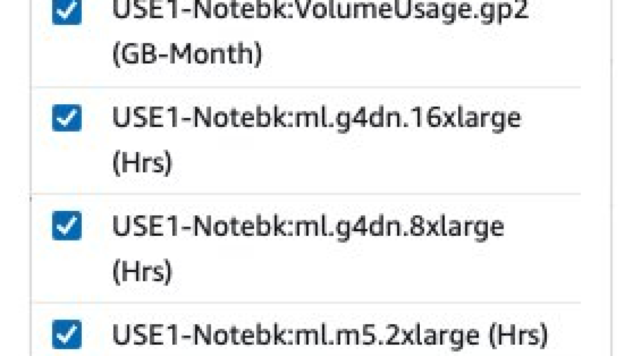
• REGION-Notebk:instanceType (for example, USE1-Notebk:ml.g4dn.8xlarge)
• REGION-Notebk:VolumeUsage.gp2 (for example, USE2-Notebk:VolumeUsage.gp2)

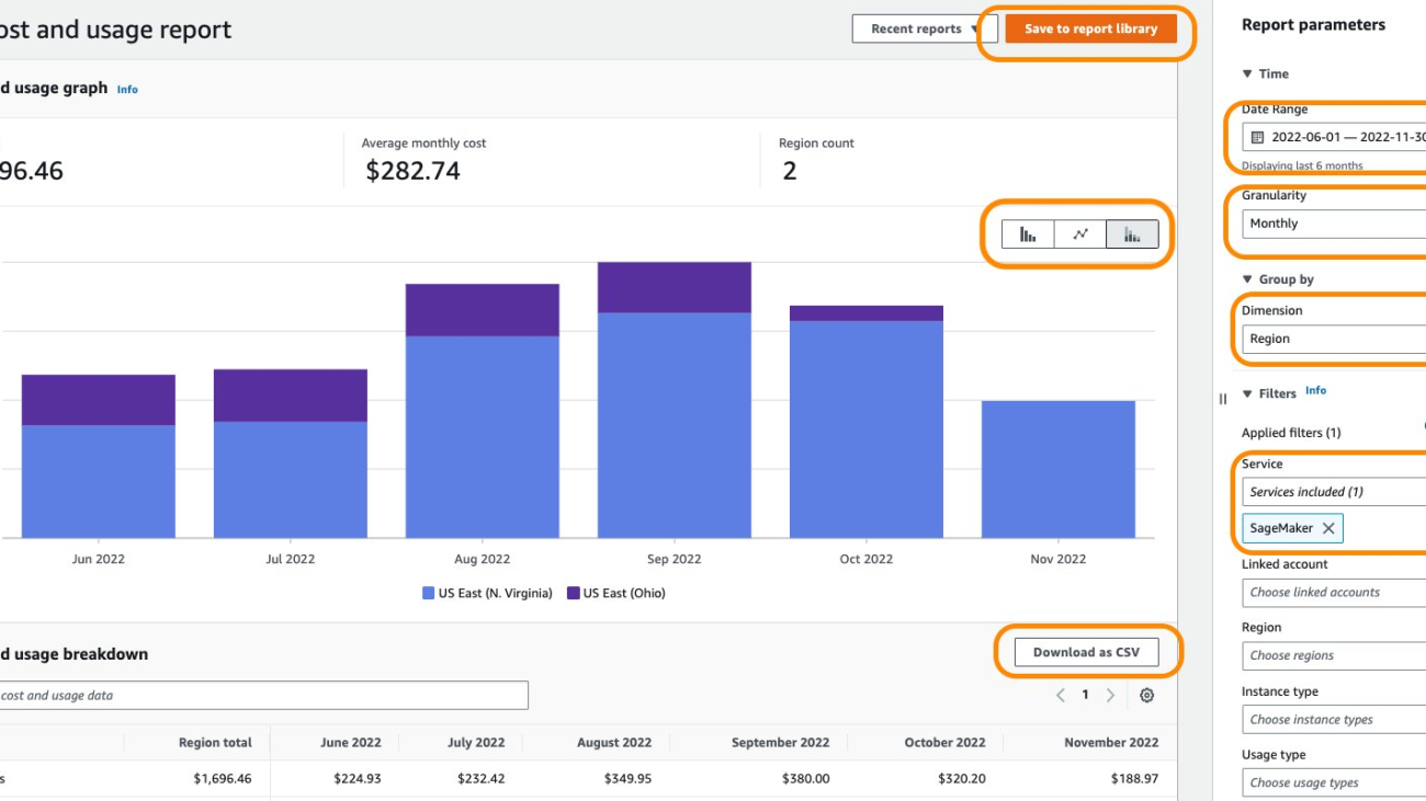
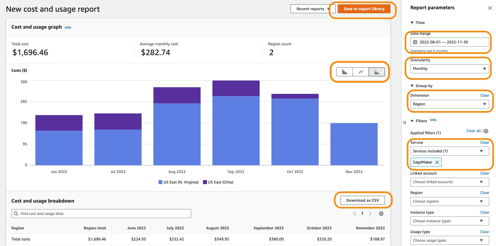
Filtering by the usage type Notebk: will show you a list of notebook usage types in an account. As shown in the following screenshot, you can select Select All and choose Apply to display the cost breakdown of your notebook usage.

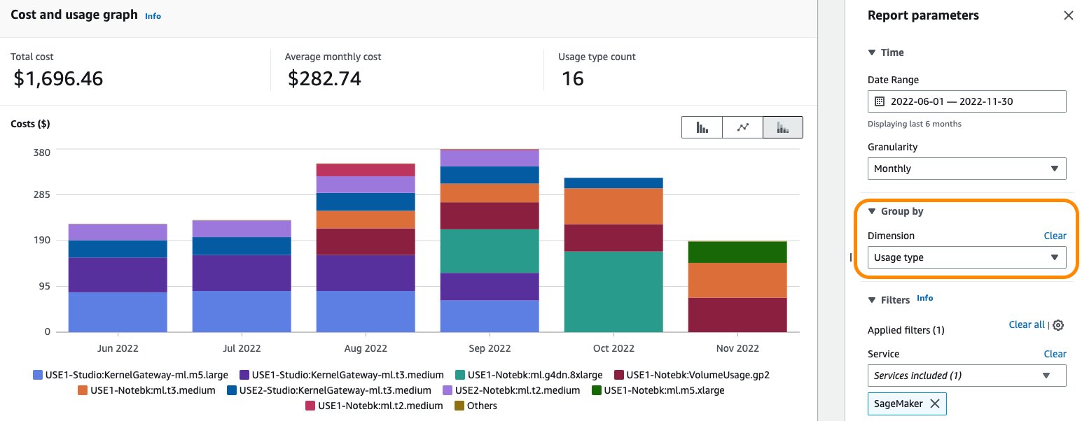
To see the cost breakdown of the selected notebook usage type by the number of usage hours, you need to de-select all the REGION-Notebk:VolumeUsage.gp2 usage types from the preceding list and choose Apply to apply the filter. The following screenshot shows the cost and usage graphs for the selected notebook usage types.

You can also apply additional filters such as account number, Amazon Elastic Compute Cloud (Amazon EC2) instance type, cost allocation tag, Region, and more. Changing the granularity to Daily gives you daily cost and usage charts based on the selected usage types and dimension, as shown in the following screenshot.

In the preceding example, the notebook instance of type ml.t2.medium in the USE2 Region is reporting a daily usage of 24 hours between the period of July 2 and September 26. Similarly, the notebook instance of type ml.t3.medium in the USE1 Region is reporting a daily usage of 24 hours between August 3 and September 26, and a daily usage of 48 hours between September 26 and December 31. Daily usage of 24 hours or more for multiple consecutive days could indicate that a notebook instance has been left running for multiple days but is not in active use. This type of pattern could benefit from applying cost control guardrails such as manual or auto-shutdown of notebook instances to prevent idle runtime.

Although Cost Explorer helps you understand cost and usage data at the granularity of the instance type, you can use AWS Cost and Usage Reports (AWS CUR) to get data at the granularity of a resource such as notebook ARN. You can build custom queries to look up AWS CUR data using standard SQL. You can also include cost-allocation tags in your query for an additional level of granularity. The following query returns notebook resource usage for the last 3 months from your AWS CUR data:

SELECT
      bill_payer_account_id,
      line_item_usage_account_id,
      line_item_resource_id AS notebook_arn,
      line_item_usage_type,
      DATE_FORMAT((line_item_usage_start_date),'%Y-%m-%d') AS day_line_item_usage_start_date,
      SUM(CAST(line_item_usage_amount AS DOUBLE)) AS sum_line_item_usage_amount,
      line_item_unblended_rate,
      SUM(CAST(line_item_unblended_cost AS DECIMAL(16,8))) AS sum_line_item_unblended_cost,
      line_item_blended_rate,
      SUM(CAST(line_item_blended_cost AS DECIMAL(16,8))) AS sum_line_item_blended_cost,
      line_item_line_item_description,
      line_item_line_item_type
    FROM 
      {$table_name}
    WHERE
      line_item_usage_start_date >= date_trunc('month',current_date - interval '3' month)
      AND line_item_product_code = 'AmazonSageMaker'
      AND line_item_line_item_type  IN ('DiscountedUsage', 'Usage', 'SavingsPlanCoveredUsage')
      AND line_item_usage_type like '%Notebk%'
        AND line_item_operation = 'RunInstance'
        AND bill_payer_account_id = 'xxxxxxxxxxxx'
    GROUP BY
      bill_payer_account_id, 
      line_item_usage_account_id,
      line_item_resource_id,
      line_item_usage_type,
      line_item_unblended_rate,
      line_item_blended_rate,
      line_item_line_item_type,
      DATE_FORMAT((line_item_usage_start_date),'%Y-%m-%d'),
      line_item_line_item_description
      ORDER BY 
      line_item_resource_id, day_line_item_usage_start_date

The following screenshot shows the results obtained from running the AWS CUR query using Amazon Athena. For more information about using Athena, refer to Querying Cost and Usage Reports using Amazon Athena.

The result of the query shows that notebook dev-notebook running on an ml.t2.medium instance is reporting 24 hours of usage for multiple consecutive days. The instance rate is $0.0464/hour and the daily cost for running for 24 hours is $1.1136.

AWS CUR query results can help you identify patterns of notebooks running for consecutive days, which can be analyzed for cost optimization. More information and example queries can be found in the AWS CUR Query Library.

You can also feed AWS CUR data into Amazon QuickSight, where you can slice and dice it any way you’d like for reporting or visualization purposes. For instructions on ingesting AWS CUR data into QuickSight, see How do I ingest and visualize the AWS Cost and Usage Report (CUR) into Amazon QuickSight.

Optimize notebook instance cost

SageMaker notebooks are suitable for ML model development, which includes interactive data exploration, script writing, prototyping of feature engineering, and modeling. Each of these tasks may have varying computing resource requirements. Estimating the right type of computing resources to serve various workloads is challenging, and may lead to over-provisioning of resources, resulting in increased cost.

For ML model development, the size of a SageMaker notebook instance depends on the amount of data you need to load in-memory for meaningful exploratory data analyses (EDA) and the amount of computation required. We recommend starting small with general-purpose instances (such as T or M families) and scaling up as needed. For example, ml.t2.medium is sufficient for most basic data processing, feature engineering, and EDA that deals with small datasets that can be held within 4 GB memory. If your model development involves heavy computational work (such as image processing), you can stop your smaller notebook instance and change the instance type to the desired larger instance, such as ml.c5.xlarge. You can switch back to the smaller instance when you no longer need a larger instance. This will help keep the compute costs down.

Consider the following best practices to help reduce the cost of your notebook instances.

CPU vs. GPU

Considering CPU vs. GPU notebook instances is important for instance right-sizing. CPUs are best at handling single, more complex calculations sequentially, whereas GPUs are better at handling multiple but simple calculations in parallel. For many use cases, a standard current generation instance type from an instance family such as M provides enough computing power, memory, and network performance for notebooks to perform well.

GPUs provide a great price/performance ratio if you take advantage of them effectively. For example, if you are training your deep learning model on a SageMaker notebook and your neural network is relatively big, performing a large number of calculations involving hundreds of thousands of parameters, then your model can take advantage of the accelerated compute and hardware parallelism offered by GPU instances such as P instance families. However, it’s recommended to use GPU instances only when you really need them because they’re expensive and GPU communication overhead might even degrade performance if your notebook doesn’t need them. We recommend using notebooks with instances that are smaller in compute for interactive building and leaving the heavy lifting to ephemeral training, tuning, and processing jobs with larger instances, including GPU-enabled instances. This way, you don’t keep a large instance (or a GPU) constantly running with your notebook. If you need accelerated computing in your notebook environment, you can stop your m* family notebook instance, switch to a GPU-enabled P* family instance, and start it again. Don’t forget to switch it back when you no longer need that extra boost in your development environment.

Restrict user access to specific instance types

Administrators can restrict users from creating notebooks that are too large through AWS Identity and Access Management (IAM) policies. For example, the following sample policy only allows users to create smaller t3 SageMaker notebook instances:

{
    "Action": [
        "sagemaker:CreateNotebookInstances"
    ],
    "Resource": [
        "*"
    ],
    "Effect": "Deny",
    "Sid": "BlockLargeNotebookInstances",
    "Condition": {
        "ForAnyValue:StringNotLike": {
            "sagemaker:InstanceTypes": [
                "ml.t3.medium",
                "ml.t3.large"
            ]
        }
    }
}

Administrators can also use AWS Service Catalog to allow for self-service of SageMaker notebooks. This allows you to restrict the instance types that are available to users when creating a notebook. For more information, see Enable self-service, secured data science using Amazon SageMaker notebooks and AWS Service Catalog and Launch Amazon SageMaker Studio using AWS Service Catalog and AWS SSO in AWS Control Tower Environment.

Stop idle notebook instances

To keep your costs down, we recommend stopping your notebook instances when you don’t need them and starting them when you do need them. Consider auto-detecting idle notebook instances and managing their lifecycle using a lifecycle configuration script. For example, auto-stop-idle is a sample shell script that stops a SageMaker notebook when it’s idle for more than 1 hour.

AWS maintains a public repository of notebook lifecycle configuration scripts that address common use cases for customizing notebook instances, including a sample bash script for stopping idle notebooks.

Schedule automatic start and stop of notebook instances

Another approach to save on notebooks cost is to automatically start and stop your notebooks at specific times. You can accomplish this by using Amazon EventBridge rules and AWS Lambda functions. For more information about configuring your Lambda functions, see Configuring Lambda function options. After you have created the functions, you can create rules to trigger these functions on a specific schedule, for example, start the notebooks every weekday at 7:00 AM. See Creating an Amazon EventBridge rule that runs on a schedule for instructions. For the scripts to start and stop notebooks with a Lambda function, refer to Ensure efficient compute resources on Amazon SageMaker.

SageMaker Studio

Studio provides a fully managed solution for data scientists to interactively build, train, and deploy ML models. Studio notebooks are one-click collaborative Jupyter notebooks that can be spun up quickly because you don’t need to set up compute instances and file storage beforehand. You are charged for the compute instance type you choose to run your notebooks on, based on the duration of use. There is no additional charge for using Studio. The costs incurred for running Studio notebooks, interactive shells, consoles, and terminals are based on ML compute instance usage.

When launched, the resource is run on an ML compute instance of the chosen instance type. If an instance of that type was previously launched and is available, the resource is run on that instance. For CPU-based images, the default suggested instance type is ml.t3.medium. For GPU-based images, the default suggested instance type is ml.g4dn.xlarge. Billing occurs per instance and starts when the first instance of a given instance type is launched.

If you want to create or open a notebook without the risk of incurring charges, open the notebook from the File menu and choose No Kernel from the Select Kernel dialog. You can read and edit a notebook without a running kernel, but you can’t run cells. You are billed separately for each instance. Billing ends when all the KernelGateway apps on the instance are shut down, or the instance is shut down. For information about billing along with pricing examples, see Amazon SageMaker Pricing.

In Cost Explorer, you can filter Studio notebook costs by applying a filter on Usage type. The name of this usage types is structured as: REGION-studio:KernelGateway-instanceType (for example, USE1-Studio:KernelGateway-ml.m5.large)

Filtering by the usage type studio: in Cost Explorer will show you the list of Studio usage types in an account. You can select the necessary usage types, or select Select All and choose Apply to display the cost breakdown of Studio app usage. The following screenshot shows the selection all the studio usage types for cost analysis.

You can also apply additional filters such as Region, linked account, or instance type for more granular cost analysis. Changing the granularity to Daily gives you daily cost and usage charts based selected usage types and dimension, as shown in the following screenshot.

In the preceding example, the Studio KernelGateway instance of type ml.t3.medium in the USE1 Region is reporting a daily usage of 48 hours between the period of January 1 and January 24, followed by a daily usage of 24 hours until February 11. Similarly, Studio KernelGateway instance of type ml.m5.large in USE1 Region is reporting 24 hours of daily usage of between January 1 and January 23. A daily usage of 24 hours or more for multiple consecutive days indicates a possibility of Studio notebook instances running continuously for multiple days. This type of pattern could benefit from applying cost control guardrails such as manual or automatic shutdown of Studio apps when not in use.

As mentioned earlier, you can use AWS CUR to get data at the granularity of a resource and build custom queries to look up AWS CUR data using standard SQL. You can also include cost-allocation tags in your query for an additional level of granularity. The following query returns Studio KernelGateway resource usage for the last 3 months from your AWS CUR data:

SELECT
      bill_payer_account_id,
      line_item_usage_account_id,
      line_item_resource_id AS studio_notebook_arn,
      line_item_usage_type,
      DATE_FORMAT((line_item_usage_start_date),'%Y-%m-%d') AS day_line_item_usage_start_date,
      SUM(CAST(line_item_usage_amount AS DOUBLE)) AS sum_line_item_usage_amount,
      line_item_unblended_rate,
      SUM(CAST(line_item_unblended_cost AS DECIMAL(16,8))) AS sum_line_item_unblended_cost,
      line_item_blended_rate,
      SUM(CAST(line_item_blended_cost AS DECIMAL(16,8))) AS sum_line_item_blended_cost,
      line_item_line_item_description,
      line_item_line_item_type
    FROM 
      customer_all
    WHERE
      line_item_usage_start_date >= date_trunc('month',current_date - interval '3' month)
      AND line_item_product_code = 'AmazonSageMaker'
      AND line_item_line_item_type  IN ('DiscountedUsage', 'Usage', 'SavingsPlanCoveredUsage')
      AND line_item_usage_type like '%Studio:KernelGateway%'
        AND line_item_operation = 'RunInstance'
        AND bill_payer_account_id = 'xxxxxxxxxxxx'
    GROUP BY
      bill_payer_account_id, 
      line_item_usage_account_id,
      line_item_resource_id,
      line_item_usage_type,
      line_item_unblended_rate,
      line_item_blended_rate,
      line_item_line_item_type,
      DATE_FORMAT((line_item_usage_start_date),'%Y-%m-%d'),
      line_item_line_item_description
      ORDER BY 
      line_item_resource_id, day_line_item_usage_start_date

The following screenshot shows the results obtained from running the AWS CUR query using Athena.

The result of the query shows that the Studio KernelGateway app named datascience-1-0-ml-t3-medium-1abf3407f667f989be9d86559395 running in account 111111111111, Studio domain d-domain1234, and user profile user1 on an ml.t3.medium instance is reporting 24 hours of usage for multiple consecutive days. The instance rate is $0.05/hour and the daily cost for running for 24 hours is $1.20.

AWS CUR query results can help you identify patterns of resources running for consecutive days at a granular level of hourly or daily usage, which can be analyzed for cost optimization. As with SageMaker notebooks, you can also feed AWS CUR data into QuickSight for reporting or visualization purposes.

SageMaker Data Wrangler

Amazon SageMaker Data Wrangler is a feature of Studio that helps you simplify the process of data preparation and feature engineering from a low-code visual interface. The usage type name for a Studio Data Wrangler app is structured as REGION-Studio_DW:KernelGateway-instanceType (for example, USE1-Studio_DW:KernelGateway-ml.m5.4xlarge).

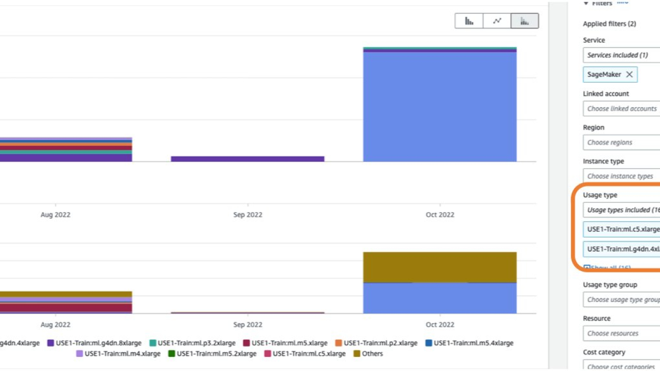
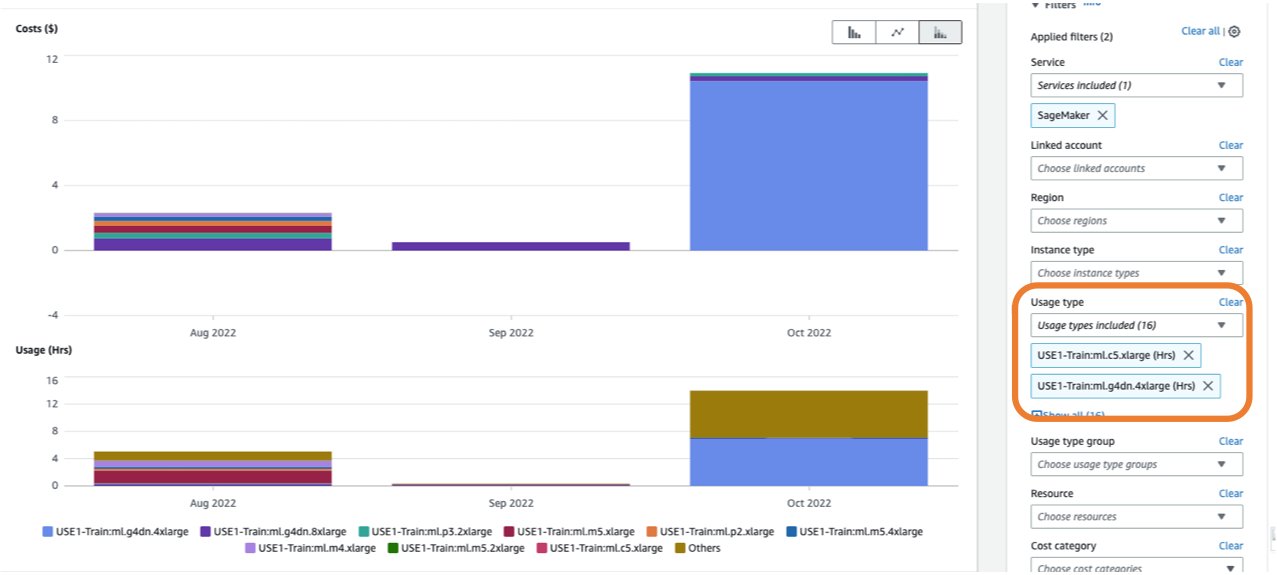
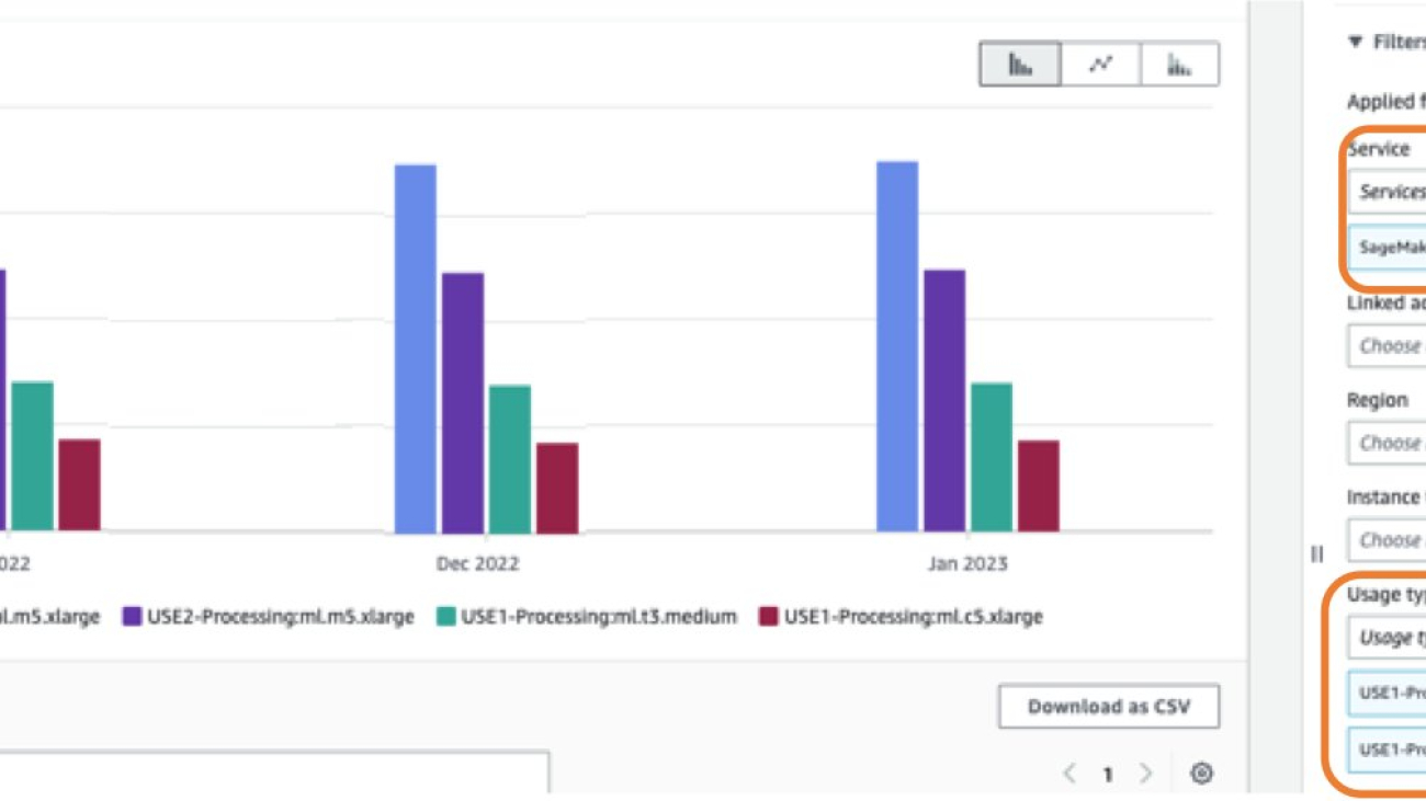
Filtering by the usage type studio_DW: in Cost Explorer will show you the list of Studio Data Wrangler usage types in an account. You can select the necessary usage types, or select Select All and choose Apply to display the cost breakdown of Studio Data Wrangler app usage. The following screenshot shows the selection all the studio_DW usage types for cost analysis.

As noted earlier, you can also apply additional filters for more granular cost analysis. For example, the following screenshot shows 24 hours of daily usage of the Studio Data Wrangler instance type ml.m5.4xlarge in the USE1 Region for multiple days and its associated cost. Insights like this can be used to apply cost control measures such as shutting down Studio apps when not in use.

You can obtain resource-level information from AWS CUR, and build custom queries to look up AWS CUR data using standard SQL. The following query returns Studio Data Wrangler app resource usage and associated cost for the last 3 months from your AWS CUR data:

SELECT
      bill_payer_account_id,
      line_item_usage_account_id,
      line_item_resource_id AS studio_notebook_arn,
      line_item_usage_type,
      DATE_FORMAT((line_item_usage_start_date),'%Y-%m-%d') AS day_line_item_usage_start_date,
      SUM(CAST(line_item_usage_amount AS DOUBLE)) AS sum_line_item_usage_amount,
      line_item_unblended_rate,
      SUM(CAST(line_item_unblended_cost AS DECIMAL(16,8))) AS sum_line_item_unblended_cost,
      line_item_blended_rate,
      SUM(CAST(line_item_blended_cost AS DECIMAL(16,8))) AS sum_line_item_blended_cost,
      line_item_line_item_description,
      line_item_line_item_type
    FROM 
      {$table_name}
    WHERE
      line_item_usage_start_date >= date_trunc('month',current_date - interval '3' month)
      AND line_item_product_code = 'AmazonSageMaker'
      AND line_item_line_item_type  IN ('DiscountedUsage', 'Usage', 'SavingsPlanCoveredUsage')
      AND line_item_usage_type like '%Studio_DW:KernelGateway%'
        AND line_item_operation = 'RunInstance'
        AND bill_payer_account_id = 'xxxxxxxxxxxx'
    GROUP BY
      bill_payer_account_id, 
      line_item_usage_account_id,
      line_item_resource_id,
      line_item_usage_type,
      line_item_unblended_rate,
      line_item_blended_rate,
      line_item_line_item_type,
      DATE_FORMAT((line_item_usage_start_date),'%Y-%m-%d'),
      line_item_line_item_description
      ORDER BY 
      line_item_resource_id, day_line_item_usage_start_date

The following screenshot shows the results obtained from running the AWS CUR query using Athena.

The result of the query shows that the Studio Data Wrangler app named sagemaker-data-wrang-ml-m5-4xlarge-b741c1a025d542c78bb538373f2d running in account 111111111111, Studio domain d-domain1234, and user profile user1 on an ml.m5.4xlarge instance is reporting 24 hours of usage for multiple consecutive days. The instance rate is $0.922/hour and the daily cost for running for 24 hours is $22.128.

Optimize Studio cost

Studio notebooks are charged for the instance type you choose, based on the duration of use. You must shut down the instance to stop incurring charges. If you shut down the notebook running on the instance but don’t shut down the instance, you will still incur charges. When you shut down the Studio notebook instances, any additional resources, such as SageMaker endpoints, Amazon EMR clusters, and Amazon Simple Storage Service (Amazon S3) buckets created from Studio are not deleted. Delete those resources if they are no longer needed to stop accrual of charges. For more details about shutting down Studio resources, refer to Shut Down Resources. If you’re using Data Wrangler, it’s important to shut it down after your work is done to save cost. For details, refer to Shut Down Data Wrangler.

Consider the following best practices to help reduce the cost of your Studio notebooks.

Automatically stop idle Studio notebook instances

You can automatically stop idle Studio notebook resources with lifecycle configurations in Studio. You can also install and use a JupyterLab extension available on GitHub as a Studio lifecycle configuration. For detailed instructions on the Studio architecture and adding the extension, see Save costs by automatically shutting down idle resources within Amazon SageMaker Studio.

Resize on the fly

The benefit of Studio notebooks over notebook instances is that with Studio, the underlying compute resources are fully elastic and you can change the instance on the fly. This allows you to scale the compute up and down as your compute demand changes, for example from ml.t3.medium to ml.m5.4xlarge, without interrupting your work or managing infrastructure. Moving from one instance to another is seamless, and you can continue working while the instance launches. With on-demand notebook instances, you need to stop the instance, update the setting, and restart with the new instance type. For more information, see Learn how to select ML instances on the fly in Amazon SageMaker Studio.

Restrict user access to specific instance types

Administrators can use IAM condition keys as an effective way to restrict certain instance types, such as GPU instances, for specific users, thereby controlling costs. For example, in the following sample policy, access is denied for all instances except ml.t3.medium and ml.g4dn.xlarge. Note that you need to allow the system instance for the default Jupyter Server apps.

{
    "Action": [
        "sagemaker:CreateApp"
    ],
    "Resource": [
        "*"
    ],
    "Effect": "Deny",
    "Sid": "BlockSagemakerLargeInstances",
    "Condition": {
        "ForAnyValue:StringNotLike": {
            "sagemaker:InstanceTypes": [
                "ml.t3.medium",
                "ml.g4dn.xlarge",
                "system"
            ]
        }
    }
}

For comprehensive guidance on best practices to optimize Studio cost, refer to Ensure efficient compute resources on Amazon SageMaker.

Use tags to keep track of Studio cost

In Studio, you can assign custom tags to your Studio domain as well as users who are provisioned access to the domain. Studio will automatically copy and assign these tags to the Studio notebooks created by the users, so you can easily track and categorize the cost of Studio notebooks and create cost chargeback models for your organization.

By default, SageMaker automatically tags new SageMaker resources such as training jobs, processing jobs, experiments, pipelines, and model registry entries with their respective sagemaker:domain-arn. SageMaker also tags the resource with the sagemaker:user-profile-arn or sagemaker:space-arn to designate the resource creation at an even more granular level.

Administrators can use automated tagging to easily monitor costs associated with their line of business, teams, individual users, or individual business problems by using tools such as AWS Budgets and Cost Explorer. For example, you can attach a cost allocation tag for the sagemaker:domain-arn tag.

This allows you to utilize Cost Explorer to visualize the Studio notebook spend for a given domain.

Consider storage costs

When the first member of your team onboards to Studio, SageMaker creates an Amazon Elastic File System (Amazon EFS) volume for the team. When this member, or any member of the team, opens Studio, a home directory is created in the volume for the member. A storage charge is incurred for this directory. Subsequently, additional storage charges are incurred for the notebooks and data files stored in the member’s home directory. For more information, see Amazon EFS Pricing.

Conclusion

In this post, we provided guidance on cost analysis and best practices when building ML models using notebook instances and Studio. As machine learning establishes itself as a powerful tool across industries, training and running ML models needs to remain cost-effective. SageMaker offers a wide and deep feature set for facilitating each step in the ML pipeline and provides cost optimization opportunities without impacting performance or agility.

About the Authors

Deepali Rajale is a Senior AI/ML Specialist at AWS. She works with enterprise customers providing technical guidance with best practices for deploying and maintaining AI/ML solutions in the AWS ecosystem. She has worked with a wide range of organizations on various deep learning use cases involving NLP and computer vision. She is passionate about empowering organizations to leverage generative AI to enhance their use experience. In her spare time, she enjoys movies, music, and literature.

Uri Rosenberg is the AI & ML Specialist Technical Manager for Europe, Middle East, and Africa. Based out of Israel, Uri works to empower enterprise customers on all things ML to design, build, and operate at scale. In his spare time, he enjoys cycling, hiking, breakfast, lunch and dinner.

Read More

Cost optimization is one of the pillars of the AWS Well-Architected Framework, and it’s a continual process of refinement and improvement over the span of a workload’s lifecycle. It enables building and operating cost-aware systems that minimize costs, maximize return on investment, and achieve business outcomes.

Amazon SageMaker is a fully managed machine learning (ML) service that offers a variety of cost optimization options and capabilities like managed spot training, multi-model endpoints, AWS Inferentia, ML Savings Plans, and many others that help reduce the total cost of ownership (TCO) of ML workloads compared to other cloud-based options, such as self-managed Amazon Elastic Compute Cloud (Amazon EC2) and AWS-managed Amazon Elastic Kubernetes Service (Amazon EKS).

AWS is dedicated to helping you achieve the highest savings by offering extensive service and pricing options. We provide tools for flexible cost management and improved visibility of detailed cost and usage of your workloads.

In 2021, we launched AWS Support Proactive Services as part of the AWS Enterprise Support plan. Since its introduction, we’ve helped hundreds of customers optimize their workloads, set guardrails, and improve the visibility of their ML workloads’ cost and usage.

In this post, we share lessons learned and walk you through the various ways to analyze your SageMaker usage and identify opportunities for cost optimization.

Analyze SageMaker cost using AWS Cost Explorer

AWS Cost Explorer provides preconfigured views that display information about your cost trends and give you a head start on understanding your cost history and trends. It allows you to filter and group by values such as AWS service, usage type, cost allocation tags, EC2 instance type, and more. If you use consolidated billing, you can also filter by linked account. In addition, you can set time intervals and granularity, as well as forecast future costs based on your historical cost and usage data.

Let’s start by using Cost Explorer to identify cost optimization opportunities in SageMaker.

1. On the Cost Explorer console, choose SageMaker for Service and choose Apply filters.
2. You can set the desired time interval and granularity, as well as the Group by parameter.
3. You can display the chart data in bar, line, or stack plot format.
4. After you have achieved your desired results with filters and groupings, you can either download your results by choosing Download as CSV or save the report by choosing Save to report library.

The following screenshot shows SageMaker costs per month for the selected date range, grouped by Region.

For general guidance on using Cost Explorer, refer to AWS Cost Explorer’s New Look and Common Use Cases.

Optionally, you can enable AWS Cost and Usage Reports (AWS CUR) to gain insights into the cost and usage data for your accounts. The report contains hourly AWS consumption details. It is stored in Amazon Simple Storage Service (Amazon S3) in the payer account, which consolidates data for all the linked accounts. You can query the report to analyze trends in your usage and take appropriate action to optimize cost. Amazon Athena is a serverless query service you can use to analyze the data from your report in Amazon S3 using standard SQL. For more information and example queries, refer to the AWS CUR Query Library.

The following code is an example of an AWS CUR query to obtain SageMaker costs for the last 3 months of usage:

SELECT *
FROM {$table_name}
WHERE 
    line_item_usage_start_date >= date_trunc('month',current_date - interval '3' month)
    AND line_item_product_code = 'AmazonSageMaker'
    AND line_item_line_item_type  IN ('DiscountedUsage', 'Usage', 'SavingsPlanCoveredUsage')

You can also feed AWS CUR data into Amazon QuickSight, where you can slice and dice it any way you’d like for reporting or visualization purposes. For instructions on ingesting CUR data into QuickSight, see How do I ingest and visualize the AWS Cost and Usage Report (CUR) into Amazon QuickSight.

Analyze cost for SageMaker usage types

Your monthly SageMaker cost comes from different SageMaker usage types such as notebook instances, hosting, training, and processing, among others. Selecting the SageMaker service filter and grouping by the Usage type dimension in Cost Explorer gives you a general idea of cost distribution based on SageMaker usage type. The usage type is displayed in the format

REGION-UsageType:instanceType (for example, USE1-Notebk:ml.g4dn.8xlarge)

The following screenshot shows cost distribution grouped by SageMaker usage types when an account has reported usage on notebooks and Amazon SageMaker Studio KernelGateway apps.

General best practices for optimizing SageMaker cost

In this section, we share general recommendations to save on costs while using SageMaker.

Tagging

A tag is a label that you assign to an AWS resource. You can use tags to organize your resources by users, departments, or cost centers, and track your costs on a detailed level. Cost allocation tags can be used for categorizing costs in Cost Explorer or Cost and Usage Reports. For tips and best practices regarding cost allocation for your SageMaker environment and workloads, refer to Set up enterprise-level cost allocation for ML environments and workloads using resource tagging in Amazon SageMaker

AWS Budgets

AWS Budgets gives you visibility into your ML cost on AWS and helps you track your SageMaker cost, including development, training, and hosting. It lets you set custom budgets to track your cost and usage from the simplest to the most complex use cases. AWS Budgets also supports email or Amazon Simple Notification Service (Amazon SNS) notification when actual or forecasted cost and usage exceeds your budget threshold, or when your actual Savings Plans’ utilization or coverage drops below your desired threshold.

AWS Budgets is also integrated with Cost Explorer, so you can easily view and analyze your cost and usage drivers, AWS Chatbot, so you can receive AWS Budget alerts in your designated Slack channel or Amazon Chime room, and AWS Service Catalog, so you can track cost on your approved AWS portfolios and products. You can also set alerts and get a notification when your cost or usage exceeds (or is forecasted to exceed) your budgeted amount. After you create your budget, you can track the progress on the AWS Budgets console. For more information, see Managing your costs with AWS Budgets.

AWS Billing console

The AWS Billing console allows you to easily understand your AWS spending, view and pay invoices, manage billing preferences and tax settings, and access additional cloud financial management services. You can quickly evaluate whether your monthly spend is in line with prior periods, forecast, or budget, and investigate and take corrective actions in a timely manner. You can use the dashboard page of the AWS Billing console to gain a general view of your AWS spending. You can also use it to identify your highest cost service or Region and view trends in your spending over the past few months as well as to see various breakdowns of your AWS usage.

The AWS summary section of the page gives an overview of your AWS costs across all accounts, Regions, service providers, and services, and other KPIs. It also provides a comparison to your total forecasted costs for the current month. The Highest cost section shows your top service, account, or Region by estimated month-to-date (MTD) spend. The Cost trend by top five services section shows the cost trend for your top five services for the most recent three to six closed billing periods.

Planning and forecasting

Forecasting is an essential part of staying on top of your cloud costs and usage, and becomes even more important as your business scales.

AWS has multiple options to help you forecast your costs. The forecasting feature of Cost Explorer gives you the ability to create custom usage forecasts to gain a line of sight into your expected future costs. The built-in ML-powered forecasting of QuickSight allows you to forecast your key business metrics with point-and-click simplicity. It offers a straightforward way to use ML to make predictions on any time series data with minimal setup time and no ML experience required.

You can also use Amazon Forecast, a fully managed service that uses ML to deliver highly accurate forecasts, to generate forecasts for specific AWS services with data collected from AWS CUR. For more information, see Forecasting AWS spend using the AWS Cost and Usage Reports, AWS Glue DataBrew, and Amazon Forecast.

For additional information about cost forecasting options, see Using the right tools for your cloud cost forecasting.

Instance right-sizing

You can optimize SageMaker cost and only pay for what you really need by selecting the right resources. You should right-size the SageMaker compute instances before purchasing a Savings Plan in order to provide a proper commitment and obtain maximum cost savings. SageMaker currently offers ML compute instances on the various instance families. Machine learning is an iterative process with varying compute requirements for different stages of the ML lifecycle, from data preprocessing to model training and model hosting. Identifying the right type of compute instance is challenging, and may lead to over-provisioning of resources and therefore increased cost. The modular architecture of SageMaker allows you to optimize the scalability, performance, and pricing of your ML workloads based on the stage of the ML lifecycle. For more details, refer to the Right-sizing compute resources for Amazon SageMaker notebooks, processing jobs, training, and deployment section of the post Ensure efficient compute resources on Amazon SageMaker.

Amazon SageMaker Savings Plans

Amazon SageMaker Savings Plans is a flexible pricing model for SageMaker. It offers discounted rates in exchange for a commitment to a consistent amount of usage (measured in $/hour) for a 1-year or 3-year term. Savings Plans provide flexibility due to their usage-based model and help reduce your costs by up to 64%. These rates automatically apply to eligible SageMaker ML instance usages including Studio notebooks, SageMaker notebook instances, SageMaker Processing, SageMaker Data Wrangler, SageMaker training, SageMaker real-time inference, and SageMaker batch transform regardless of instance family, size, or Region. This makes it easy for you to maximize savings regardless of how your use cases and consumption evolve over time, and you can save up to 64% compared to the On-Demand price.

For example, you could start with small instances to experiment with different algorithms on a fraction of your dataset. Then, you could move to larger instances to prepare data and train at scale against your full dataset. Finally, you could deploy your models in several Regions to serve low-latency predictions to your users. All the instance size modifications and deployments across new Regions would be covered by the same Savings Plan, without any management effort required on your part.

Every type of SageMaker usage that is eligible for SageMaker Savings Plans has a Savings Plans rate and an On-Demand rate. When you sign up for the SageMaker Savings Plans, you will be charged the Savings Plan rate for your usage up to your commitment. Any usage beyond the commitment will be charged at On-Demand rates. The AWS Cost Management console provides you with recommendations that make it easy to find the right commitment level for a Savings Plan. These recommendations are based on the following:

• Your SageMaker usage in the last 7, 30, or 60 days. You should select the time period that best represents your future usage.
• The term of your plan: 1-year or 3-year.
• Your payment option: No Upfront, Partial Upfront (50% or more), or All Upfront. Some customers prefer (or must use) this last option, because it gives them a clear and predictable view of their SageMaker bill.

The recommendations are based on your historical usage over the selected lookback period and don’t forecast your usage. Be sure to select a lookback period that reflects your future usage. A 3-year term plan provides the highest discount rate; similarly, an All Upfront payment option offers the highest discount rate compared to No Upfront or Partial Upfront payment options. Workloads and usage typically change over time and a consistent, steady-state usage pattern makes a good candidate for a savings plan. If you have a lot of short-lived or one-off workloads, selecting the right commitment for compute usage (measured per hour) could be difficult. It’s recommended to continually purchase small amounts of Savings Plans commitment over time. This ensures that you maintain high levels of coverage to maximize your discounts, and your plans closely match your workload and organization requirements at all times.

To understand Savings Plan recommendations, refer to Decrease Your Machine Learning Costs with Instance Price Reductions and Savings Plans for Amazon SageMaker.

Utilization report

For active Savings Plans, utilization reports are available on the Savings Plans console to see the percentage of the commitment that you’ve actually used. You can use your Savings Plans utilization report to visually understand how much of your Savings Plans commitment you are using over the configured time period, as well as your savings as compared to On-Demand prices. For example, if you have a $10/hour commitment, and your usage billed with Savings Plans rates totals to $9.80 for the hour, your utilization for that hour is 98%. You can see your Savings Plans utilization at an hourly, daily, or monthly granularity, based on your lookback period. You can apply filters by Savings Plans type, member account, Region, and instance family in the Filters section. If you’re a user in a management account, you can see the aggregated utilization for the entire Consolidated Billing Family.

The following screenshot shows an example of a utilization report. You can see that even though Savings Plans coverage is not 100% on many consecutive days, the total net savings is still positive. Without Savings Plans, you would be charged at On-Demand rates for the usage. To realize maximum savings and avoid over-committing, it’s recommended to select the right commitment based on consistent, optimized usage of your SageMaker workloads.

Coverage report

Likewise, coverage reports show you how much of your eligible spend has been covered by the plan. To understand how the coverage is calculated, refer to Using your coverage report.

The following screenshot shows an example of a coverage report. You can see that the average coverage for the selected time period is 92%, along with the On-Demand spend that was not covered by the plan. Based on the On-Demand spend not covered by the plan, you can optionally buy an additional Savings Plan to obtain maximum savings. Also, it’s recommended to right-size the SageMaker compute instances before purchasing a Savings Plan and understand the workload size to avoid over- or under-committing the Savings Plan usage.

For more details on how Savings Plans apply to your AWS usage, refer to Understanding how Savings Plans apply to your AWS usage.

Conclusion

Machine learning has established itself as a powerful tool across industries, but training new models and running ML models for inference can be costly. One of the advantages of running ML on SageMaker is the wide and deep feature set offering cost optimization strategies without impacting performance or agility. This post highlighted the AWS tools and options to analyze your SageMaker costs, identify trends, and implement proactive alerts and optimization best practices.

About the Authors

Deepali Rajale is a Senior AI/ML Specialist at AWS. She works with enterprise customers providing technical guidance with best practices for deploying and maintaining AI/ML solutions in the AWS ecosystem. She has worked with a wide range of organizations on various deep learning use cases involving NLP and computer vision. She is passionate about empowering organizations to leverage generative AI to enhance their use experience. In her spare time, she enjoys movies, music, and literature.

Uri Rosenberg is the AI & ML Specialist Technical Manager for Europe, Middle East, and Africa. Based out of Israel, Uri works to empower enterprise customers on all things ML to design, build, and operate at scale. In his spare time, he enjoys cycling, hiking, and time traveling.

Read More

Amazon SageMaker Ground Truth Plus helps you prepare high-quality training datasets by removing the undifferentiated heavy lifting associated with building data labeling applications and managing the labeling workforce. All you do is share data along with labeling requirements, and Ground Truth Plus sets up and manages your data labeling workflow based on these requirements. From there, an expert workforce that is trained on a variety of machine learning (ML) tasks labels your data. You don’t even need deep ML expertise or knowledge of workflow design and quality management to use Ground Truth Plus. Now, Ground Truth Plus is serving customers who need data labeling and human feedback for fine-tuning foundation models for generative AI applications.

In this post, you will learn about recent advancements in human feedback for generative AI available through SageMaker Ground Truth Plus. This includes new workflows and user interfaces (UIs) available for preparing demonstration datasets used in supervised fine-tuning, gathering high-quality human feedback to make preference datasets for aligning generative AI foundation models with human preferences, as well as customizing models to application builders’ requirements for style, substance, and voice.

Challenges of getting started with generative AI

Generative AI applications around the world incorporate both single-mode and multi-modal foundation models to solve for many different use cases. Common among them are chatbots, image generators, and video generators. Large language models (LLMs) are being used in chatbots for creative pursuits, academic and personal assistants, business intelligence tools, and productivity tools. You can use text-to-image models to generate abstract or realistic AI art and marketing assets. Text-to-video models are being used to generate videos for art projects, highly engaging advertisements, video game development, and even film development.

Two of the most important problems to solve for both model producers who create foundation models and application builders who use existing generative foundation models to build their own tools and applications are:

• Fine-tuning these foundation models to be able to perform specific tasks
• Aligning them with human preferences to ensure they output helpful, accurate, and harmless information

Foundation models are typically pre-trained on large corpora of unlabeled data, and therefore don’t perform well following natural language instructions. For an LLM, that means that they may be able to parse and generate language in general, but they may not be able to answer questions coherently or summarize text up to a user’s required quality. For example, when a user requests a summary of a text in a prompt, a model that hasn’t been fine-tuned how to summarize text may just recite the prompt text back to the user or respond with something irrelevant. If a user asks a question about a topic, the response from a model could just be a recitation of the question. For multi-modal models, such as text-to-image or text-to-video models, the models may output content unrelated to the prompt. For example, if a corporate graphic designer prompts a text-to-image model to create a new logo or an image for an advertisement, the model may not generate a relevant graphic related to the prompt if it has only a general concept of an image and elements of an image. In some cases, a model may output a harmful image or video, risking user confidence or company reputation.

Even if models are fine-tuned to perform specific tasks, they may not be aligned with human preferences with respect to the meaning, style, or substance of their output content. In an LLM, this could manifest itself as inaccurate or even harmful content being generated by the model. For example, a model that isn’t aligned with human preferences through fine-tuning may output dangerous, unethical, or even illegal instructions when prompted by a user. No care will have been taken to limit the content being generated by the model to ensure it is aligned with human preferences to be accurate, relevant, and useful. This misalignment can be a problem for companies that rely on generative AI models for their applications, such as chatbots and multimedia creation. For multi-modal models, this may take the form of toxic, dangerous, or abusive images or video being generated. This is a risk when prompts are input to the model without the intention of generating sensitive content, and also if the model producer or application builder had not intended to allow the model to generate that kind of content, but it was generated anyway.

To solve the issues of task-specific capability and aligning generative foundation models with human preferences, model producers and application builders must fine-tune the models with data using human-directed demonstrations and human feedback of model outputs.

Data and training types

There are several types of fine-tuning methods with different types of labeled data that are categorized as instruction tuning – or teaching a model how to follow instructions. Among them are supervised fine-tuning (SFT) using demonstration data, and reinforcement learning from human feedback (RLHF) using preference data.

Demonstration data for supervised fine-tuning

To fine-tune foundation models to perform specific tasks such as answering questions or summarizing text with high quality, the models undergo SFT with demonstration data. The purpose of demonstration data is to guide the model by providing it with labeled examples (demonstrations) of completed tasks being done by humans. For example, to teach an LLM how to answer questions, a human annotator will create a labeled dataset of human-generated question and answer pairs to demonstrate how a question and answer interaction works linguistically and what the content means semantically. This kind of SFT trains the model to recognize patterns of behavior demonstrated by the humans in the demonstration training data. Model producers need to do this type of fine-tuning to show that their models are capable of performing such tasks for downstream adopters. Application builders who use existing foundation models for their generative AI applications may need to fine-tune their models with demonstration data on these tasks with industry-specific or company-specific data to improve the relevancy and accuracy of their applications.

Preference data for instruction tuning such as RLHF

To further align foundation models with human preferences, model producers—and especially application builders—need to generate preference datasets to perform instruction tuning. Preference data in the context of instruction tuning is labeled data that captures human feedback with respect to a set of options output by a generative foundation model. It typically includes rating or ranking several inferences or pairwise comparing two inferences from a foundation model according to some specific attribute. For LLMs, these attributes may be helpfulness, accuracy, and harmlessness. For text-to-image models, it may be an aesthetic quality or text-image alignment. This preference data based on human feedback can then be used in various instruction tuning methods—including RLHF—in order to further fine-tune a model to align with human preferences.

Instruction tuning using preference data plays a crucial role in enhancing the personalization and effectiveness of foundation models. This is a key step in building custom applications on top of pre-trained foundation models and is a powerful method to ensure models are generating helpful, accurate, and harmless content. A common example of instruction tuning is to instruct a chatbot to generate three responses to a query, and have a human read and rank all three according to some specified dimension, such as toxicity, factual accuracy, or readability. For example, a company may use a chatbot for its marketing department and wants to make sure that content is aligned to its brand message, doesn’t exhibit biases, and is clearly readable. The company would prompt the chatbot during instruction tuning to produce three examples, and have their internal experts select the ones that most align to their goal. Over time, they build a dataset used to teach the model what style of content humans prefer through reinforcement learning. This enables the chatbot application to output more relevant, readable, and safe content.

SageMaker Ground Truth Plus

Ground Truth Plus helps you address both challenges—generating demonstration datasets with task-specific capabilities, as well as gathering preference datasets from human feedback to align models with human preferences. You can request projects for LLMs and multi-modal models such as text-to-image and text-to-video. For LLMs, key demonstration datasets include generating questions and answers (Q&A), text summarization, text generation, and text reworking for the purposes of content moderation, style change, or length change. Key LLM preference datasets include ranking and classifying text outputs. For multi-modal models, key task types include captioning images or videos as well as logging timestamps of events in videos. Therefore, Ground Truth Plus can help both model producers and application builders on their generative AI journey.

In this post, we dive deeper into the human annotator and feedback journey on four cases covering both demonstration data and preference data for both LLMs and multi-modal models: question and answer pair generation and text ranking for LLMs, as well as image captioning and video captioning for multi-modal models.

Large language models

In this section, we discuss question and answer pairs and text ranking for LLMs, along with customizations you may want for your use case.

Question and answer pairs

The following screenshot shows a labeling UI in which a human annotator will read a text passage and generate both questions and answers in the process of building a Q&A demonstration dataset.

Let’s walk through a tour of the UI in the annotator’s shoes. On the left side of the UI, the job requester’s specific instructions are presented to the annotator. In this case, the annotator is supposed to read the passage of text presented in the center of the UI and create questions and answers based on the text. On the right side, the questions and answers that the annotator has written are shown. The text passage as well as type, length, and number of questions and answers can all be customized by the job requester during the project setup with the Ground Truth Plus team. In this case, the annotator has created a question that requires understanding the whole text passage to answer and is marked with a References entire passage check box. The other two questions and answers are based on specific parts of the text passage, as shown by the annotator highlights with color-coded matching. Optionally, you may want to request that questions and answers are generated without a provided text passage, and provide other guidelines for human annotators—this is also supported by Ground Truth Plus.

After the questions and answers are submitted, they can flow to an optional quality control loop workflow where other human reviewers will confirm that customer-defined distribution and types of questions and answers have been created. If there is a mismatch between the customer requirements and what the human annotator has produced, the work will get funneled back to a human for rework before being exported as part of the dataset to deliver to the customer. When the dataset is delivered back to you, it’s ready to incorporate into the supervised fine-tuning workflow at your discretion.

Text ranking

The following screenshot shows a UI for ranking the outputs from an LLM based on a prompt.

You can simply write the instructions for the human reviewer, and bring prompts and pre-generated responses to the Ground Truth Plus project team to start the job. In this case, we have requested for a human reviewer to rank three responses per prompt from an LLM on the dimension of writing clarity (readability). Again, the left pane shows the instructions given to the reviewer by the job requester. In the center, the prompt is at the top of the page, and the three pre-generated responses are the main body for ease of use. On the right side of the UI, the human reviewer will rank them in order of most to least clear writing.

Customers wanting to generate this type of preference dataset include application builders interested in building human-like chatbots, and therefore want to customize the instructions for their own use. The length of the prompt, number of responses, and ranking dimension can all be customized. For example, you may want to rank five responses in order of most to least factually accurate, biased, or toxic, or even rank and classify multiple dimensions simultaneously. These customizations are supported in Ground Truth Plus.

Multi-modal models

In this section, we discuss image and video captioning for training multi-modal models such as text-to-image and text-to-video models, as well as customizations you may want to make for your particular use case.

Image captioning

The following screenshot shows a labeling UI for image captioning. You can request a project with image captioning to gather data to train a text-to-image model or an image-to-text model.

In this case, we have requested to train a text-to-image model and have set specific requirements on the caption in terms of length and detail. The UI is designed to walk the human annotators through the cognitive process of generating rich captions by providing a mental framework through assistive and descriptive tools. We have found that providing this mental framework for annotators results in more descriptive and accurate captions than simply providing an editable text box alone.

The first step in the framework is for the human annotator to identify key objects in the image. When the annotator chooses an object in the image, a color-coded dot appears on the object. In this case, the annotator has chosen both the dog and the cat, creating two editable fields on the right side of the UI wherein the annotator will enter the names of the objects—cat and dog—along with a detailed description of each object. Next, the annotator is guided to identify all the relationships between all the objects in the image. In this case, the cat is relaxing next to the dog. Next, the annotator is asked to identify specific attributes about the image, such as the setting, background, or environment. Finally, in the caption input text box, the annotator is instructed to combine all of what they wrote in the objects, relationships, and image setting fields into a complete single descriptive caption of the image.

Optionally, you can configure this image caption to be passed through a human-based quality check loop with specific instructions to ensure that the caption meets the requirements. If there is an issue identified, such as a missing key object, that caption can be sent back for a human to correct the issue before exporting as part of the training dataset.

Video captioning

The following screenshot shows a video captioning UI to generate rich video captions with timestamp tags. You can request a video caption project to gather data to build text-to-video or video-to-text models.

In this labeling UI, we have built a similar mental framework to ensure high-quality captions are written. The human annotator can control the video on the left side and create descriptions and timestamps for each activity shown in the video on the right side with the UI elements. Similar to the image captioning UI, there is also a place for the annotator to write a detailed description of the video setting, background, and environment. Finally, the annotator is instructed to combine all the elements into a coherent video caption.

Similar to the image caption case, the video captions may optionally flow through a human-based quality control workflow to determine if your requirements are met. If there is an issue with the video captions, it will be sent for rework by the human annotator workforce.

Conclusion

Ground Truth Plus can help you prepare high-quality datasets to fine-tune foundation models for generative AI tasks, from answering questions to generating images and videos. It also allows skilled human workforces to review model outputs to ensure that they are aligned with human preferences. Additionally, it enables application builders to customize models using their industry or company data to ensure their application represents their preferred voice and style. These are the first of many innovations in Ground Truth Plus, and more are in development. Stay tuned for future posts.

Interested in starting a project to build or improve your generative AI models and applications? Get started with Ground Truth Plus by connecting with our team today.

About the authors

Jesse Manders is a Senior Product Manager in the AWS AI/ML human in the loop services team. He works at the intersection of AI and human interaction with the goal of creating and improving AI/ML products and services to meet our needs. Previously, Jesse held leadership roles in engineering at Apple and Lumileds, and was a senior scientist in a Silicon Valley startup. He has an M.S. and Ph.D. from the University of Florida, and an MBA from the University of California, Berkeley, Haas School of Business.

Romi Datta is a Senior Manager of Product Management in the Amazon SageMaker team responsible for Human in the Loop services. He has been in AWS for over 4 years, holding several product management leadership roles in SageMaker, S3 and IoT. Prior to AWS he worked in various product management, engineering and operational leadership roles at IBM, Texas Instruments and Nvidia. He has an M.S. and Ph.D. in Electrical and Computer Engineering from the University of Texas at Austin, and an MBA from the University of Chicago Booth School of Business.

Jonathan Buck is a Software Engineer at Amazon Web Services working at the intersection of machine learning and distributed systems. His work involves productionizing machine learning models and developing novel software applications powered by machine learning to put the latest capabilities in the hands of customers.

Alex Williams is an applied scientist in the human-in-the-loop science team at AWS AI where he conducts interactive systems research at the intersection of human-computer interaction (HCI) and machine learning. Before joining Amazon, he was a professor in the Department of Electrical Engineering and Computer Science at the University of Tennessee where he co-directed the People, Agents, Interactions, and Systems (PAIRS) research laboratory. He has also held research positions at Microsoft Research, Mozilla Research, and the University of Oxford. He regularly publishes his work at premier publication venues for HCI, such as CHI, CSCW, and UIST. He holds a PhD from the University of Waterloo.

Sarah Gao is a Software Development Manager in Amazon SageMaker Human In the Loop (HIL) responsible for building the ML based labeling platform. Sarah has been in AWS for over 4 years, holding several software management leadership roles in EC2 security and SageMaker. Prior to AWS she worked in various engineering management roles at Oracle and Sun Microsystem.

Erran Li is the applied science manager at human-in-the-loop services, AWS AI, Amazon. His research interests are 3D deep learning, and vision and language representation learning. Previously he was a senior scientist at Alexa AI, the head of machine learning at Scale AI and the chief scientist at Pony.ai. Before that, he was with the perception team at Uber ATG and the machine learning platform team at Uber working on machine learning for autonomous driving, machine learning systems and strategic initiatives of AI. He started his career at Bell Labs and was adjunct professor at Columbia University. He co-taught tutorials at ICML’17 and ICCV’19, and co-organized several workshops at NeurIPS, ICML, CVPR, ICCV on machine learning for autonomous driving, 3D vision and robotics, machine learning systems and adversarial machine learning. He has a PhD in computer science at Cornell University. He is an ACM Fellow and IEEE Fellow.

Read More

Text-to-image generation is a task in which a machine learning (ML) model generates an image from a textual description. The goal is to generate an image that closely matches the description, capturing the details and nuances of the text. This task is challenging because it requires the model to understand the semantics and syntax of the text and to generate photorealistic images. There are many practical applications of text-to-image generation in AI photography, concept art, building architecture, fashion, video games, graphic design, and much more.

Stable Diffusion is a text-to-image model that empowers you to create high-quality images within seconds. When real-time interaction with this type of model is the goal, ensuring a smooth user experience depends on the use of accelerated hardware for inference, such as GPUs or AWS Inferentia2, Amazon’s own ML inference accelerator. The steep costs involved in using GPUs typically requires optimizing the utilization of the underlying compute, even more so when you need to deploy different architectures or personalized (fine-tuned) models. Amazon SageMaker multi-model endpoints (MMEs) help you address this problem by helping you scale thousands of models into one endpoint. By using a shared serving container, you can host multiple models in a cost-effective, scalable manner within the same endpoint, and even the same GPU.

In this post, you will learn about Stable Diffusion model architectures, different types of Stable Diffusion models, and techniques to enhance image quality. We also show you how to deploy Stable Diffusion models cost-effectively using SageMaker MMEs and NVIDIA Triton Inference Server.

Prompt: portrait of a cute bernese dog, art by elke Vogelsang, 8k ultra realistic, trending on artstation, 4 k	Prompt: architecture design of living room, 8 k ultra-realistic, 4 k, hyperrealistic, focused, extreme details	Prompt: New York skyline at night, 8k, long shot photography, unreal engine 5, cinematic, masterpiece

Stable Diffusion architecture

Stable Diffusion is a text-to-image open-source model that you can use to create images of different styles and content simply by providing a text prompt. In the context of text-to-image generation, a diffusion model is a generative model that you can use to generate high-quality images from textual descriptions. Diffusion models are a type of generative model that can capture the complex dependencies between the input and output modalities text and images.

The following diagram shows a high-level architecture of a Stable Diffusion model.

It consists of the following key elements:

• Text encoder – CLIP is a transformers-based text encoder model that takes input prompt text and converts it into token embeddings that represent each word in the text. CLIP is trained on a dataset of images and their captions, a combination of image encoder and text encoder.
• U-Net – A U-Net model takes token embeddings from CLIP along with an array of noisy inputs and produces a denoised output. This happens though a series of iterative steps, where each step processes an input latent tensor and produces a new latent space tensor that better represents the input text.
• Auto encoder-decoder – This model creates the final images. It takes the final denoised latent output from the U-Net model and converts it into images that represents the text input.

Types of Stable Diffusion models

In this post, we explore the following pre-trained Stable Diffusion models by Stability AI from the Hugging Face model hub.

stable-diffusion-2-1-base

Use this model to generate images based on a text prompt. This is a base version of the model that was trained on LAION-5B. The model was trained on a subset of the large-scale dataset LAION-5B, and mainly with English captions. We use StableDiffusionPipeline from the diffusers library to generate images from text prompts. This model can create images of dimension 512 x 512. It uses the following parameters:

• prompt – A prompt can be a text word, phrase, sentences, or paragraphs.
• negative_prompt – You can also pass a negative prompt to exclude specified elements from the image generation process and to enhance the quality of the generated images.
• guidance_scale – A higher guidance scale results in an image more closely related to the prompt, at the expense of image quality. If specified, it must be a float.

stable-diffusion-2-depth

This model is used to generate new images from existing ones while preserving the shape and depth of the objects in the original image. This stable-diffusion-2-depth model is fine-tuned from stable-diffusion-2-base, an extra input channel to process the (relative) depth prediction. We use StableDiffusionDepth2ImgPipeline from the diffusers library to load the pipeline and generate depth images. The following are the additional parameters specific to the depth model:

• image – The initial image to condition the generation of new images.
• num_inference_steps (optional) – The number of denoising steps. More denoising steps usually leads to a higher-quality image at the expense of slower inference. This parameter is modulated by strength.
• strength (optional) – Conceptually, this indicates how much to transform the reference image. The value must be between 0–1. image is used as a starting point, adding more noise to it the larger the strength. The number of denoising steps depends on the amount of noise initially added. When strength is 1, the added noise will be maximum and the denoising process will run for the full number of iterations specified in num_inference_steps. A value of 1, therefore, essentially ignores image. For more details, refer to the following code.

stable-diffusion-2-inpainting

You can use this model for AI image restoration use cases. You can also use it to create novel designs and images from the prompts and additional arguments. This model is also derived from the base model and has a mask generation strategy. It specifies the mask of the original image to represent segments to be changed and segments to leave unchanged. We use StableDiffusionUpscalePipeline from the diffusers library to apply inpaint changes on original image. The following additional parameter is specific to the depth model:

• mask_input – An image where the blacked-out portion remains unchanged during image generation and the white portion is replaced

stable-diffusion-x4-upscaler

This model is also derived from the base model, additionally trained on the 10M subset of LAION containing 2048 x 2048 images. As the name implies, it can be used to upscale lower-resolution images to higher resolutions

Use case overview

For this post, we deploy an AI image service with multiple capabilities, including generating novel images from text, changing the styles of existing images, removing unwanted objects from images, and upscaling low-resolution images to higher resolutions. Using several variations of Stable Diffusion models, you can address all of these use cases within a single SageMaker endpoint. This means that you’ll need to host large number of models in a performant, scalable, and cost-efficient way. In this post, we show how to deploy multiple Stable Diffusion models cost-effectively using SageMaker MMEs and NVIDIA Triton Inference Server. You will learn about the implementation details, optimization techniques, and best practices to work with text-to-image models.

The following table summarizes the Stable Diffusion models that we deploy to a SageMaker MME.

Solution overview

The following steps are involved in deploying Stable Diffusion models to SageMaker MMEs:

1. Use the Hugging Face hub to download the Stable Diffusion models to a local directory. This will download scheduler, text_encoder, tokenizer, unet, and vae for each Stable Diffusion model into its corresponding local directory. We use the revision="fp16" version of the model.
2. Set up the NVIDIA Triton model repository, model configurations, and model serving logic model.py. Triton uses these artifacts to serve predictions.
3. Package the conda environment with additional dependencies and the package model repository to be deployed to the SageMaker MME.
4. Package the model artifacts in an NVIDIA Triton-specific format and upload model.tar.gz to Amazon Simple Storage Service (Amazon S3). The model will be used for generating images.
5. Configure a SageMaker model, endpoint configuration, and deploy the SageMaker MME.
6. Run inference and send prompts to the SageMaker endpoint to generate images using the Stable Diffusion model. We specify the TargetModel variable and invoke different Stable Diffusion models to compare the results visually.

We have published the code to implement this solution architecture in the GitHub repo. Follow the README instructions to get started.

Serve models with an NVIDIA Triton Inference Server Python backend

We use a Triton Python backend to deploy the Stable Diffusion pipeline model to a SageMaker MME. The Python backend lets you serve models written in Python by Triton Inference Server. To use the Python backend, you need to create a Python file model.py that has the following structure: Every Python backend can implement four main functions in the TritonPythonModel class:

import triton_python_backend_utils as pb_utils
class TritonPythonModel:
"""Your Python model must use the same class name. Every Python model
that is created must have "TritonPythonModel" as the class name.
"""
def auto_complete_config(auto_complete_model_config):
def initialize(self, args):
def execute(self, requests):
def finalize(self):

Every Python backend can implement four main functions in the TritonPythonModel class: auto_complete_config, initialize, execute, and finalize.

initialize is called when the model is being loaded. Implementing initialize is optional. initialize allows you to do any necessary initializations before running inference. In the initialize function, we create a pipeline and load the pipelines using from_pretrained checkpoints. We configure schedulers from the pipeline scheduler config pipe.scheduler.config. Finally, we specify xformers optimizations to enable the xformer memory efficient parameter enable_xformers_memory_efficient_attention. We provide more details on xformers later in this post. You can refer to model.py of each model to understand the different pipeline details. This file can be found in the model repository.

The execute function is called whenever an inference request is made. Every Python model must implement the execute function. In the execute function, you are given a list of InferenceRequest objects. We pass the input text prompt to the pipeline to get an image from the model. Images are decoded and the generated image is returned from this function call.

We get the input tensor from the name defined in the model configuration config.pbtxt file. From the inference request, we get prompt, negative_prompt, and gen_args, and decode them. We pass all the arguments to the model pipeline object. Encode the image to return the generated image predictions. You can refer to the config.pbtxt file of each model to understand the different pipeline details. This file can be found in the model repository. Finally, we wrap the generated image in InferenceResponse and return the response.

Implementing finalize is optional. This function allows you to do any cleanups necessary before the model is unloaded from Triton Inference Server.

When working with the Python backend, it’s the user’s responsibility to ensure that the inputs are processed in a batched manner and that responses are sent back accordingly. To achieve this, we recommend following these steps:

1. Loop through all requests in the requests object to form a batched_input.
2. Run inference on the batched_input.
3. Split the results into multiple InferenceResponse objects and concatenate them as the responses.

Refer to the Triton Python backend documentation or Host ML models on Amazon SageMaker using Triton: Python backend for more details.

NVIDIA Triton model repository and configuration

The model repository contains the model serving script, model artifacts and tokenizer artifacts, a packaged conda environment (with dependencies needed for inference), the Triton config file, and the Python script used for inference. The latter is mandatory when you use the Python backend, and you should use the Python file model.py. Let’s explore the configuration file of the inpaint Stable Diffusion model and understand the different options specified:

name: "sd_inpaint"
backend: "python"
max_batch_size: 8
input [
  {
    name: "prompt"
    data_type: TYPE_STRING
    dims: [
      -1
    ]
  },
  {
    name: "negative_prompt"
    data_type: TYPE_STRING
    dims: [
      -1
    ]
    optional: true
  },
  {
    name: "image"
    data_type: TYPE_STRING
    dims: [
      -1
    ]
  },
  {
    name: "mask_image"
    data_type: TYPE_STRING
    dims: [
      -1
    ]
  },
  {
    name: "gen_args"
    data_type: TYPE_STRING
    dims: [
      -1
    ]
    optional: true
  }
]
output [
  {
    name: "generated_image"
    data_type: TYPE_STRING    
    dims: [
      -1
    ]
  }
]
instance_group [
  {
    kind: KIND_GPU
  }
]
parameters: {
  key: "EXECUTION_ENV_PATH",
  value: {string_value: "/tmp/conda/sd_env.tar.gz"
  }
}

The following table explains the various parameters and values:

For details about the model repository and configurations of other Stable Diffusion models, refer to the code in the GitHub repo. Each directory contains artifacts for the specific Stable Diffusion models.

Package a conda environment and extend the SageMaker Triton container

SageMaker NVIDIA Triton container images don’t contain libraries like transformer, accelerate, and diffusers to deploy and serve Stable Diffusion models. However, Triton allows you to bring additional dependencies using conda-pack. Let’s start by creating the conda environment with the necessary dependencies outlined in the environment.yml file and create a tar model artifact sd_env.tar.gz file containing the conda environment with dependencies installed in it. Run the following YML file to create a conda-pack artifact and copy the artifact to the local directory from where it will be uploaded to Amazon S3. Note that we will be uploading the conda artifacts as one of the models in the MME and invoking this model to set up the conda environment in the SageMaker hosting ML instance.

%%writefile environment.yml
name: mme_env
dependencies:
  - python=3.8
  - pip
  - pip:
      - numpy
      - torch --extra-index-url https://download.pytorch.org/whl/cu118
      - accelerate
      - transformers
      - diffusers
      - xformers
      - conda-pack

!conda env create -f environment.yml –force

Upload model artifacts to Amazon S3

SageMaker expects the .tar.gz file containing each Triton model repository to be hosted on the multi-model endpoint. Therefore, we create a tar artifact with content from the Triton model repository. We can use this S3 bucket to host thousands of model artifacts, and the SageMaker MME will use models from this location to dynamically load and serve a large number of models. We store all the Stable Diffusion models in this Amazon S3 location.

Deploy the SageMaker MME

In this section, we walk through the steps to deploy the SageMaker MME by defining container specification, SageMaker model and endpoint configurations.

Define the serving container

In the container definition, define the ModelDataUrl to specify the S3 directory that contains all the models that the SageMaker MME will use to load and serve predictions. Set Mode to MultiModel to indicate that SageMaker will create the endpoint with the MME container specifications. We set the container with an image that supports deploying MMEs with GPU. See Supported algorithms, frameworks, and instances for more details.

We see all three model artifacts in the following Amazon S3 ModelDataUrl location:

container = {"Image": mme_triton_image_uri, 
             "ModelDataUrl": model_data_url, 
             "Mode": "MultiModel"}

Create an MME object

We use the SageMaker Boto3 client to create the model using the create_model API. We pass the container definition to the create model API along with ModelName and ExecutionRoleArn:

create_model_response = sm_client.create_model(
    ModelName=sm_model_name, 
    ExecutionRoleArn=role, 
    PrimaryContainer=container
)

Define configurations for the MME

Create an MME configuration using the create_endpoint_config Boto3 API. Specify an accelerated GPU computing instance in InstanceType (we use the same instance type that we are using to host our SageMaker notebook). We recommend configuring your endpoints with at least two instances with real-life use cases. This allows SageMaker to provide a highly available set of predictions across multiple Availability Zones for the models.

create_endpoint_config_response = sm_client.create_endpoint_config(
    EndpointConfigName=endpoint_config_name,
    ProductionVariants=[
        {
            "InstanceType": instance_type,
            "InitialVariantWeight": 1,
            "InitialInstanceCount": 1,
            "ModelName": sm_model_name,
            "VariantName": "AllTraffic",
        }
    ],
)

Create an MME

Use the preceding endpoint configuration to create a new SageMaker endpoint and wait for the deployment to finish:

create_endpoint_response = sm_client.create_endpoint(
                EndpointName=endpoint_name, 
                EndpointConfigName=endpoint_config_name
)

The status will change to InService when the deployment is successful.

Generate images using different versions of Stable Diffusion models

Let’s start by invoking the base model with a prompt and getting the generated image. We pass the inputs to the base model with prompt, negative_prompt, and gen_args as a dictionary. We set the data type and shape of each input item in the dictionary and pass it as input to the model.

inputs = dict(prompt = "Infinity pool on top of a high rise overlooking Central Park",
             negative_prompt = "blur,low detail, low quality",
             gen_args = json.dumps(dict(num_inference_steps=50, guidance_scale=8))
)
payload = {
    "inputs":
        [{"name": name, "shape": [1,1], "datatype": "BYTES", "data": [data]} for name, data in inputs.items()]
}
response = runtime_sm_client.invoke_endpoint(
        EndpointName=endpoint_name,
        ContentType="application/octet-stream",
        Body=json.dumps(payload),
        TargetModel="sd_base.tar.gz", 
    )
output = json.loads(response["Body"].read().decode("utf8"))["outputs"]
decode_image(output[0]["data"][0])

Prompt: Infinity pool on top of a high rise overlooking Central Park

Working with this image, we can modify it with the versatile Stable Diffusion depth model. For example, we can change the style of the image to an oil painting, or change the setting from Central Park to Yellowstone National Park simply by passing the original image along with a prompt describing the changes we would like to see.

We invoke the depth model by specifying sd_depth.tar.gz in the TargetModel of the invoke_endpoint function call. In the outputs, notice how the orientation of the original image is preserved, but for one example, the NYC buildings have been transformed into rock formations of the same shape.

inputs = dict(prompt = "highly detailed oil painting of an inifinity pool overlooking central park",
              image=image,
              gen_args = json.dumps(dict(num_inference_steps=50, strength=0.9))
              )
payload = {
    "inputs":
        [{"name": name, "shape": [1,1], "datatype": "BYTES", "data": [data]} for name, data in inputs.items()]
}
response = runtime_sm_client.invoke_endpoint(
        EndpointName=endpoint_name,
        ContentType="application/octet-stream",
        Body=json.dumps(payload),
        TargetModel="sd_depth.tar.gz", 
    )
output = json.loads(response["Body"].read().decode("utf8"))["outputs"]
print("original image")
display(original_image)
print("generated image")
display(decode_image(output[0]["data"][0]))

Original image	Oil painting	Yellowstone Park

Another useful model is Stable Diffusion inpainting, which we can use to remove certain parts of the image. Let’s say you want to remove the tree in the following example image. We can do so by invoking the inpaint model sd_inpaint.tar.gz. To remove the tree, we need to pass a mask_image, which indicates which regions of the image should be retained and which should be filled in. The black pixel portion of the mask image indicates the regions that should remain unchanged, and the white pixels indicate what should be replaced.

image = encode_image(original_image).decode("utf8")
mask_image = encode_image(Image.open("sample_images/bertrand-gabioud-mask.png")).decode("utf8")
inputs = dict(prompt = "building, facade, paint, windows",
              image=image,
              mask_image=mask_image,
              negative_prompt = "tree, obstruction, sky, clouds",
              gen_args = json.dumps(dict(num_inference_steps=50, guidance_scale=10))
              )
payload = {
    "inputs":
        [{"name": name, "shape": [1,1], "datatype": "BYTES", "data": [data]} for name, data in inputs.items()]
}
response = runtime_sm_client.invoke_endpoint(
        EndpointName=endpoint_name,
        ContentType="application/octet-stream",
        Body=json.dumps(payload),
        TargetModel="sd_inpaint.tar.gz", 
    )
output = json.loads(response["Body"].read().decode("utf8"))["outputs"]
decode_image(output[0]["data"][0])

Original image	Mask image	Inpaint image

In our final example, we downsize the original image that was generated earlier from its 512 x 512 resolution to 128 x 128. We then invoke the Stable Diffusion upscaler model to upscale the image back to 512 x 512. We use the same prompt to upscale the image as what we used to generate the initial image. While not necessary, providing a prompt that describes the image helps guide the upscaling process and should lead to better results.

low_res_image = output_image.resize((128, 128))
inputs = dict(prompt = "Infinity pool on top of a high rise overlooking Central Park",
             image=encode_image(low_res_image).decode("utf8")
)

payload = {
    "inputs":
        [{"name": name, "shape": [1,1], "datatype": "BYTES", "data": [data]} for name, data in inputs.items()]
}

response = runtime_sm_client.invoke_endpoint(
        EndpointName=endpoint_name,
        ContentType="application/octet-stream",
        Body=json.dumps(payload),
        TargetModel="sd_upscale.tar.gz", 
    )
output = json.loads(response["Body"].read().decode("utf8"))["outputs"]
upscaled_image = decode_image(output[0]["data"][0])

Low-resolution image	Upscaled image

Although the upscaled image is not as detailed as the original, it’s a marked improvement over the low-resolution one.

Optimize for memory and speed

The xformers library is a way to speed up image generation. This optimization is only available for NVIDIA GPUs. It speeds up image generation and lowers VRAM usage. We have used the xformers library for memory-efficient attention and speed. When the enable_xformers_memory_efficient_attention option is enabled, you should observe lower GPU memory usage and a potential speedup at inference time.

Clean Up

Follow the instruction in the clean up section of the notebook to delete the resource provisioned part of this blog to avoid unnecessary charges. Refer Amazon SageMaker Pricing for details the cost of the inference instances.

Conclusion

In this post, we discussed Stable Diffusion models and how you can deploy different versions of Stable Diffusion models cost-effectively using SageMaker multi-model endpoints. You can use this approach to build a creator image generation and editing tool. Check out the code samples in the GitHub repo to get started and let us know about the cool generative AI tool that you build.

About the Authors

Simon Zamarin is an AI/ML Solutions Architect whose main focus is helping customers extract value from their data assets. In his spare time, Simon enjoys spending time with family, reading sci-fi, and working on various DIY house projects.

Vikram Elango is a Sr. AI/ML Specialist Solutions Architect at AWS, based in Virginia, US. He is currently focused on generative AI, LLMs, prompt engineering, large model inference optimization, and scaling ML across enterprises. Vikram helps financial and insurance industry customers with design and architecture to build and deploy ML applications at scale. In his spare time, he enjoys traveling, hiking, cooking, and camping with his family.

João Moura is an AI/ML Specialist Solutions Architect at AWS, based in Spain. He helps customers with deep learning model training and inference optimization, and more broadly building large-scale ML platforms on AWS. He is also an active proponent of ML-specialized hardware and low-code ML solutions.

Saurabh Trikande is a Senior Product Manager for Amazon SageMaker Inference. He is passionate about working with customers and is motivated by the goal of democratizing machine learning. He focuses on core challenges related to deploying complex ML applications, multi-tenant ML models, cost optimizations, and making deployment of deep learning models more accessible. In his spare time, Saurabh enjoys hiking, learning about innovative technologies, following TechCrunch, and spending time with his family.

Read More

One of the most common applications of generative AI and large language models (LLMs) in an enterprise environment is answering questions based on the enterprise’s knowledge corpus. Amazon Lex provides the framework for building AI based chatbots. Pre-trained foundation models (FMs) perform well at natural language understanding (NLU) tasks such summarization, text generation and question answering on a broad variety of topics but either struggle to provide accurate (without hallucinations) answers or completely fail at answering questions about content that they haven’t seen as part of their training data. Furthermore, FMs are trained with a point in time snapshot of data and have no inherent ability to access fresh data at inference time; without this ability they might provide responses that are potentially incorrect or inadequate.

A commonly used approach to address this problem is to use a technique called Retrieval Augmented Generation (RAG). In the RAG-based approach we convert the user question into vector embeddings using an LLM and then do a similarity search for these embeddings in a pre-populated vector database holding the embeddings for the enterprise knowledge corpus. A small number of similar documents (typically three) is added as context along with the user question to the “prompt” provided to another LLM and then that LLM generates an answer to the user question using information provided as context in the prompt. RAG models were introduced by Lewis et al. in 2020 as a model where parametric memory is a pre-trained seq2seq model and the non-parametric memory is a dense vector index of Wikipedia, accessed with a pre-trained neural retriever. To understand the overall structure of a RAG-based approach, refer to Question answering using Retrieval Augmented Generation with foundation models in Amazon SageMaker JumpStart.

In this post we provide a step-by-step guide with all the building blocks for creating an enterprise ready RAG application such as a question answering bot. We use a combination of different AWS services, open-source foundation models (FLAN-T5 XXL for text generation and GPT-j-6B for embeddings) and packages such as LangChain for interfacing with all the components and Streamlit for building the bot frontend.

We provide an AWS Cloud Formation template to stand up all the resources required for building this solution. We then demonstrate how to use LangChain for tying everything together:

• Interfacing with LLMs hosted on Amazon SageMaker.
• Chunking of knowledge base documents.
• Ingesting document embeddings into Amazon OpenSearch Service.
• Implementing the question answering task.

We can use the same architecture to swap the open-source models with the Amazon Titan models. After Amazon Bedrock launches, we will publish a follow-up post showing how to implement similar generative AI applications using Amazon Bedrock, so stay tuned.

Solution overview

We use the SageMaker docs as the knowledge corpus for this post. We convert the HTML pages on this site into smaller overlapping chunks (to retain some context continuity between chunks) of information and then convert these chunks into embeddings using the gpt-j-6b model and store the embeddings in OpenSearch Service. We implement the RAG functionality inside an AWS Lambda function with Amazon API Gateway to handle routing all requests to the Lambda. We implement a chatbot application in Streamlit which invokes the function via the API Gateway and the function does a similarity search in the OpenSearch Service index for the embeddings of user question. The matching documents (chunks) are added to the prompt as context by the Lambda function and then the function uses the flan-t5-xxl model deployed as a SageMaker endpoint to generate an answer to the user question. All the code for this post is available in the GitHub repo.

The following figure represents the high-level architecture of the proposed solution.

Figure 1: Architecture

Step-by-step explanation:

1. The User provides a question via the Streamlit web application.
2. The Streamlit application invokes the API Gateway endpoint REST API.
3. The API Gateway invokes the Lambda function.
4. The function invokes the SageMaker endpoint to convert user question into embeddings.
5. The function invokes invokes an OpenSearch Service API to find similar documents to the user question.
6. The function creates a “prompt” with the user query and the “similar documents” as context and asks the SageMaker endpoint to generate a response.
7. The response is provided from the function to the API Gateway.
8. The API Gateway provides the response to the Streamlit application.
9. The User is able to view the response on the Streamlit application,

As illustrated in the architecture diagram, we use the following AWS services:

• SageMaker and Amazon SageMaker JumpStart for hosting the two LLMs.
• OpenSearch Service for storing the embeddings of the enterprise knowledge corpus and doing similarity search with user questions.
• Lambda for implementing the RAG functionality and exposing it as a REST endpoint via the API Gateway.
• Amazon SageMaker Processing jobs for large scale data ingestion into OpenSearch.
• Amazon SageMaker Studio for hosting the Streamlit application.
• AWS Identity and Access Management roles and policies for access management.
• AWS CloudFormation for creating the entire solution stack through infrastructure as code.

In terms of open-source packages used in this solution, we use LangChain for interfacing with OpenSearch Service and SageMaker, and FastAPI for implementing the REST API interface in the Lambda.

The workflow for instantiating the solution presented in this post in your own AWS account is as follows:

1. Run the CloudFormation template provided with this post in your account. This will create all the necessary infrastructure resources needed for this solution:
   • SageMaker endpoints for the LLMs
   • OpenSearch Service cluster
   • API Gateway
   • Lambda function
   • SageMaker Notebook
   • IAM roles
2. Run the data_ingestion_to_vectordb.ipynb notebook in the SageMaker notebook to ingest data from SageMaker docs into an OpenSearch Service index.
3. Run the Streamlit application on a terminal in Studio and open the URL for the application in a new browser tab.
4. Ask your questions about SageMaker via the chat interface provided by the Streamlit app and view the responses generated by the LLM.

These steps are discussed in detail in the following sections.

Prerequisites

To implement the solution provided in this post, you should have an AWS account and familiarity with LLMs, OpenSearch Service and SageMaker.

We need access to accelerated instances (GPUs) for hosting the LLMs. This solution uses one instance each of ml.g5.12xlarge and ml.g5.24xlarge; you can check the availability of these instances in your AWS account and request these instances as needed via a Sevice Quota increase request as shown in the following screenshot.

Figure 2: Service Quota Increase Request

Use AWS Cloud Formation to create the solution stack

We use AWS CloudFormation to create a SageMaker notebook called aws-llm-apps-blog and an IAM role called LLMAppsBlogIAMRole. Choose Launch Stack for the Region you want to deploy resources to. All parameters needed by the CloudFormation template have default values already filled in, except for the OpenSearch Service password which you’d have to provide. Make a note of the OpenSearch Service username and password, we use those in subsequent steps. This template takes about 15 minutes to complete.

AWS Region	Link
us-east-1
us-west-2
eu-west-1
ap-northeast-1

After the stack is created successfully, navigate to the stack’s Outputs tab on the AWS CloudFormation console and note the values for OpenSearchDomainEndpoint and LLMAppAPIEndpoint. We use those in the subsequent steps.

Figure 3: Cloud Formation Stack Outputs

Ingest the data into OpenSearch Service

To ingest the data, complete the following steps:

1. On the SageMaker console, choose Notebooks in the navigation pane.
2. Select the notebook aws-llm-apps-blog and choose Open JupyterLab.
   

   Figure 4: Open JupyterLab

3. Choose data_ingestion_to_vectordb.ipynb to open it in JupyterLab. This notebook will ingest the SageMaker docs to an OpenSearch Service index called llm_apps_workshop_embeddings.
   

   Figure 5: Open Data Ingestion Notebook

4. When the notebook is open, on the Run menu, choose Run All Cells to run the code in this notebook. This will download the dataset locally into the notebook and then ingest it into the OpenSearch Service index. This notebook takes about 20 minutes to run. The notebook also ingests the data into another vector database called FAISS. The FAISS index files are saved locally and the uploaded to Amazon Simple Storage Service (S3) so that they can optionally be used by the Lambda function as an illustration of using an alternate vector database.
   

   Figure 6: Notebook Run All Cells

Now we’re ready to split the documents into chunks, which can then be converted into embeddings to be ingested into OpenSearch. We use the LangChain RecursiveCharacterTextSplitter class to chunk the documents and then use the LangChain SagemakerEndpointEmbeddingsJumpStart class to convert these chunks into embeddings using the gpt-j-6b LLM. We store the embeddings in OpenSearch Service via the LangChain OpenSearchVectorSearch class. We package this code into Python scripts that are provided to the SageMaker Processing Job via a custom container. See the data_ingestion_to_vectordb.ipynb notebook for the full code.

5. Create a custom container, then install in it the LangChain and opensearch-py Python packages.
6. Upload this container image to Amazon Elastic Container Registry (ECR).
7. We use the SageMaker ScriptProcessor class to create a SageMaker Processing job that will run on multiple nodes.
   • The data files available in Amazon S3 are automatically distributed across in the SageMaker Processing job instances by setting s3_data_distribution_type='ShardedByS3Key' as part of the ProcessingInput provided to the processing job.
   • Each node processes a subset of the files and this brings down the overall time required to ingest the data into OpenSearch Service.
   • Each node also uses Python multiprocessing to internally also parallelize the file processing. Therefore, there are two levels of parallelization happening, one at the cluster level where individual nodes are distributing the work (files) amongst themselves and another at the node level where the files in a node are also split between multiple processes running on the node.

      # setup the ScriptProcessor with the above parameters
     processor = ScriptProcessor(base_job_name=base_job_name,
                                 image_uri=image_uri,
                                 role=aws_role,
                                 instance_type=instance_type,
                                 instance_count=instance_count,
                                 command=["python3"],
                                 tags=tags)
     
     # setup input from S3, note the ShardedByS3Key, this ensures that 
     # each instance gets a random and equal subset of the files in S3.
     inputs = [ProcessingInput(source=f"s3://{bucket}/{app_name}/{DOMAIN}",
                               destination='/opt/ml/processing/input_data',
                               s3_data_distribution_type='ShardedByS3Key',
                               s3_data_type='S3Prefix')]
     
     
     logger.info(f"creating an opensearch index with name={opensearch_index}")
     # ready to run the processing job
     st = time.time()
     processor.run(code="container/load_data_into_opensearch.py",
                   inputs=inputs,
                   outputs=[],
                   arguments=["--opensearch-cluster-domain", opensearch_domain_endpoint,
                             "--opensearch-secretid", os_creds_secretid_in_secrets_manager,
                             "--opensearch-index-name", opensearch_index,
                             "--aws-region", aws_region,
                             "--embeddings-model-endpoint-name", embeddings_model_endpoint_name,
                             "--chunk-size-for-doc-split", str(CHUNK_SIZE_FOR_DOC_SPLIT),
                             "--chunk-overlap-for-doc-split", str(CHUNK_OVERLAP_FOR_DOC_SPLIT),
                             "--input-data-dir", "/opt/ml/processing/input_data",
                             "--create-index-hint-file", CREATE_OS_INDEX_HINT_FILE,
                             "--process-count", "2"])

8. Close the notebook after all cells run without any error. Your data is now available in OpenSearch Service. Enter the following URL in your browser’s address bar to get a count of documents in the llm_apps_workshop_embeddings index. Use the OpenSearch Service domain endpoint from the CloudFormation stack outputs in the URL below. You’d be prompted for the OpenSearch Service username and password, these are available from the CloudFormations stack.

   https://your-opensearch-domain-endpoint/llm_apps_workshop_embeddings/_count

The browser window should show an output similar to the following. This output shows that 5,667 documents were ingested into the llm_apps_workshop_embeddings index. {"count":5667,"_shards":{"total":5,"successful":5,"skipped":0,"failed":0}}

Run the Streamlit application in Studio

Now we’re ready to run the Streamlit web application for our question answering bot. This application allows the user to ask a question and then fetches the answer via the /llm/rag REST API endpoint provided by the Lambda function.

Studio provides a convenient platform to host the Streamlit web application. The following steps describes how to run the Streamlit app on Studio. Alternatively, you could also follow the same procedure to run the app on your laptop.

1. Open Studio and then open a new terminal.
2. Run the following commands on the terminal to clone the code repository for this post and install the Python packages needed by the application:

   git clone https://github.com/aws-samples/llm-apps-workshop
   cd llm-apps-workshop/blogs/rag/app
   pip install -r requirements.txt

3. The API Gateway endpoint URL that is available from the CloudFormation stack output needs to be set in the webapp.py file. This is done by running the following sed command. Replace the replace-with-LLMAppAPIEndpoint-value-from-cloudformation-stack-outputs in the shell commands with the value of the LLMAppAPIEndpoint field from the CloudFormation stack output and then run the following commands to start a Streamlit app on Studio.

   
   EP=replace-with-LLMAppAPIEndpoint-value-from-cloudformation-stack-outputs
   # replace __API_GW_ENDPOINT__ with  output from the cloud formation stack
   sed -i "s|__API_GW_ENDPOINT__|$EP|g" webapp.py
   streamlit run webapp.py

4. When the application runs successfully, you’ll see an output similar to the following (the IP addresses you will see will be different from the ones shown in this example). Note the port number (typically 8501) from the output to use as part of the URL for app in the next step.

   sagemaker-user@studio$ streamlit run webapp.py 
   
   Collecting usage statistics. To deactivate, set browser.gatherUsageStats to False.
   
   You can now view your Streamlit app in your browser.
   
   Network URL: http://169.255.255.2:8501
   External URL: http://52.4.240.77:8501

5. You can access the app in a new browser tab using a URL that is similar to your Studio domain URL. For example, if your Studio URL is https://d-randomidentifier.studio.us-east-1.sagemaker.aws/jupyter/default/lab? then the URL for your Streamlit app will be https://d-randomidentifier.studio.us-east-1.sagemaker.aws/jupyter/default/proxy/8501/webapp (notice that lab is replaced with proxy/8501/webapp). If the port number noted in the previous step is different from 8501 then use that instead of 8501 in the URL for the Streamlit app.

The following screenshot shows the app with a couple of user questions.

A closer look at the RAG implementation in the Lambda function

Now that we have the application working end to end, lets take a closer look at the Lambda function. The Lambda function uses FastAPI to implement the REST API for RAG and the Mangum package to wrap the API with a handler that we package and deploy in the function. We use the API Gateway to route all incoming requests to invoke the function and handle the routing internally within our application.

The following code snippet shows how we find documents in the OpenSearch index that are similar to the user question and then create a prompt by combining the question and the similar documents. This prompt is then provided to the LLM for generating an answer to the user question.

@router.post("/rag")
async def rag_handler(req: Request) -> Dict[str, Any]:
    # dump the received request for debugging purposes
    logger.info(f"req={req}")

    # initialize vector db and SageMaker Endpoint
    _init(req)

    # Use the vector db to find similar documents to the query
    # the vector db call would automatically convert the query text
    # into embeddings
    docs = _vector_db.similarity_search(req.q, k=req.max_matching_docs)
    logger.info(f"here are the {req.max_matching_docs} closest matching docs to the query="{req.q}"")
    for d in docs:
        logger.info(f"---------")
        logger.info(d)
        logger.info(f"---------")

    # now that we have the matching docs, lets pack them as a context
    # into the prompt and ask the LLM to generate a response
    prompt_template = """Answer based on context:nn{context}nn{question}"""

    prompt = PromptTemplate(
        template=prompt_template, input_variables=["context", "question"]
    )
    logger.info(f"prompt sent to llm = "{prompt}"")
    chain = load_qa_chain(llm=_sm_llm, prompt=prompt)
    answer = chain({"input_documents": docs, "question": req.q}, return_only_outputs=True)['output_text']
    logger.info(f"answer received from llm,nquestion: "{req.q}"nanswer: "{answer}"")
    resp = {'question': req.q, 'answer': answer}
    if req.verbose is True:
        resp['docs'] = docs

    return resp

Clean up

To avoid incurring future charges, delete the resources. You can do this by deleting the CloudFormation stack as shown in the following screenshot.

Figure 7: Cleaning Up

Conclusion

In this post, we showed how to create an enterprise ready RAG solution using a combination of AWS service, open-source LLMs and open-source Python packages.

We encourage you to learn more by exploring JumpStart, Amazon Titan models, Amazon Bedrock, and OpenSearch Service and building a solution using the sample implementation provided in this post and a dataset relevant to your business. If you have questions or suggestions, leave a comment.

About the Authors

Amit Arora is an AI and ML Specialist Architect at Amazon Web Services, helping enterprise customers use cloud-based machine learning services to rapidly scale their innovations. He is also an adjunct lecturer in the MS data science and analytics program at Georgetown University in Washington D.C.

Dr. Xin Huang is a Senior Applied Scientist for Amazon SageMaker JumpStart and Amazon SageMaker built-in algorithms. He focuses on developing scalable machine learning algorithms. His research interests are in the area of natural language processing, explainable deep learning on tabular data, and robust analysis of non-parametric space-time clustering. He has published many papers in ACL, ICDM, KDD conferences, and Royal Statistical Society: Series A.

Navneet Tuteja is a Data Specialist at Amazon Web Services. Before joining AWS, Navneet worked as a facilitator for organizations seeking to modernize their data architectures and implement comprehensive AI/ML solutions. She holds an engineering degree from Thapar University, as well as a master’s degree in statistics from Texas A&M University.

Read More

Amazon Kendra is a highly accurate and intelligent search service that enables users to search unstructured and structured data using natural language processing (NLP) and advanced search algorithms. With Amazon Kendra, you can find relevant answers to your questions quickly, without sifting through documents. However, just enabling end-users to get the answers to their queries is not enough in today’s world. We need to constantly understand the end-user’s search behavior, such as what are the top queries for the month, have any new query that queries appeared recently, what percentage of queries received instant answer, and more.

Although the Amazon Kendra console comes equipped with an analytics dashboard, many of our customers prefer to build a custom dashboard. This allows you to create unique views and filters, and grants management teams access to a streamlined, one-click dashboard without needing to log in to the AWS Management Console and search for the appropriate dashboard. In addition, you can enhance your dashboard’s functionality by adding preprocessing logic, such as grouping similar top queries. For example, you may want to group similar queries such as “What is Amazon Kendra” and “What is the purpose of Amazon Kendra” together so that you can effectively analyze the metrics and gain a deeper understanding of the data. Such grouping of similar queries can be done using the concept of semantic similarity.

This post discusses an end-to-end solution to implement this use case, which includes using AWS Lambda to extract the summarized metrics from Amazon Kendra, calculating the semantic similarity score using a Hugging Face model hosted on an Amazon SageMaker Serverless Inference endpoint to group similar queries, and creating an Amazon QuickSight dashboard to display the user insights effectively.

Solution overview

The following diagram illustrates our solution architecture.

The high-level workflow is as follows:

1. An Amazon EventBridge scheduler triggers Lambda functions once a month to extract last month’s search metrics from Amazon Kendra.
2. The Lambda functions upload the search metrics to an Amazon Simple Storage Service (Amazon S3) bucket.
3. The Lambda functions group similar queries in the uploaded file based on the semantic similarity score by Hugging Face model hosted on a SageMaker inference endpoint.
4. An AWS Glue crawler creates or updates the AWS Glue Data Catalog from the uploaded file in the S3 bucket for an Amazon Athena table.
5. QuickSight uses the Athena table dataset to create analyses and dashboards.

For this solution, we deploy the infrastructure resources to create the QuickSight analysis and dashboard using an AWS CloudFormation template.

Prerequisites

Complete the following prerequisite steps:

1. If you’re a first-time user of QuickSight in your AWS account, sign up for QuickSight.
2. Get the Amazon Kendra index ID that you want visualize your search metrics from Amazon Kendra. You will have to use the search engine for a while (for example, a few weeks) to be able to extract a sufficient amount of data to use to extract some insights.
   
3. Clone the GitHub repo to create the container image:
   1. app.py
   2. Dockerfile
   3. requirements.txt
4. Create an Amazon Elastic Container Registry (Amazon ECR) repository in us-east-1 and push the container image created by the downloaded Dockerfile. For instructions, refer to Creating a private repository.
5. Run the following commands in the directory of your local environment to create and push the container image to the ECR repository you created:

aws ecr get-login-password --region us-east-1 | docker login --username AWS --password-stdin <YOUR_AWS_ACCOUNT_ID>.dkr.ecr.us-east-1.amazonaws.com
docker build -t <YOUR_ECR_REPOSITORY_NAME> .
docker tag <YOUR_ECR_REPOSITORY_NAME>:latest <YOUR_AWS_ACCOUNT_ID>.dkr.ecr.us-east-1.amazonaws.com/<YOUR_ECR_REPOSITORY_NAME>:latest 
docker push <YOUR_AWS_ACCOUNT_ID>.dkr.ecr.us-east-1.amazonaws.com/<YOUR_ECR_REPOSITORY_NAME>:latest

Deploy the CloudFormation template

Complete the following steps to deploy the CloudFormation template:

1. Download the CloudFormation template kendrablog-sam-template.yml.
2. On the AWS CloudFormation console, create a new stack.

Use the us-east-1 Region for this deployment.

3. Upload the template directly or through your preferred S3 bucket.
   
4. For KendraIndex, enter the Amazon Kendra index ID from the prerequisites.
5. For LambdaECRRepository, enter the ECR repository from the prerequisites.
6. For QSIdentityRegion, enter the identity Region of QuickSight. The identity Region aligns with your Region selection when you signed up your QuickSight subscription.
7. For QSUserDefaultPassward, enter the default password to use for your QuickSight user.

You’ll be prompted to change this password when you first sign in to the QuickSight console.

8. For QSUserEmail, enter the email address to use for the QuickSight user.
9. Choose Next.
   
10. Leave other settings as default and choose Next.
    
11. Select the acknowledgement check boxes and choose Create stack.
    

When the deployment is complete, you can confirm all the generated resources on the stack’s Resources tab on the AWS CloudFormation console.

We walk through some of the key components of this solution in the following sections.

Get insights from Amazon Kendra search metrics

We can get the metrics data from Amazon Kendra using the GetSnapshots API. There are 10 metrics for analyzing what information the users are searching for: 5 metrics include trends data for us to look for patterns over time, and 5 metrics use just a snapshot or aggregated data. The metrics with the daily trend data are clickthrough rate, zero click rate, zero search results rate, instant answer rate, and total queries. The metrics with aggregated data are top queries, top queries with zero clicks, top queries with zero search results, top clicked on documents, and total documents.

We use Lambda functions to get the search metrics data from Amazon Kendra. The functions extract the metrics from Amazon Kendra and store them in Amazon S3. You can find the functions in the GitHub repo.

Create a SageMaker serverless endpoint and host a Hugging Face model to calculate semantic similarity

After the metrics are extracted, the next step is to complete the preprocessing for the aggregated metrics. The preprocessing step checks the semantic similarity between the query texts and groups them together to show the total counts for the similar queries. For example, if there are three queries of “What is S3” and two queries of “What is the purpose of S3,” it will group them together and show that there are five queries of “What is S3” or “What is the purpose of S3.”

To calculate semantic similarity, we use a model from the Hugging Face model library. Hugging Face is a popular open-source platform that provides a wide range of NLP models, including transformers, which have been trained on a variety of NLP tasks. These models can be easily integrated with SageMaker and take advantage of its rich training and deployment options. The Hugging Face Deep Learning Containers (DLCs), which comes pre-packaged with the necessary libraries, make it easy to deploy the model in SageMaker with just few lines of code. In our use case, we first get the vector embedding using the Hugging Face pre-trained model flax-sentence-embeddings/all_datasets_v4_MiniLM-L6, and then use cosine similarity to calculate the similarity score between the vector embeddings.

To get the vector embedding from the Hugging Face model, we create a serverless endpoint in SageMaker. Serverless endpoints help save cost because you only pay for the amount of time the inference runs. To create a serverless endpoint, you first define the max concurrent invocations for a single endpoint, known as MaxConcurrency, and the memory size. The memory sizes you can choose are 1024 MB, 2048 MB, 3072 MB, 4096 MB, 5120 MB, or 6144 MB. SageMaker Serverless Inference auto-assigns compute resources proportional to the memory you select.

We also need to pad one of the vectors with zeros so that the size of the two vectors matches with each other and we can calculate the cosine similarity as a dot product of the two vectors. We can set a threshold for cosine similarity (for example, 0.6) and if the similarity score is more than the threshold, we can group the queries together. After the queries are grouped, we can understand the top queries better. We put all this logic in a Lambda function and deploy the function using a container image. The container image contains codes to invoke the SageMaker Serverless Inference endpoints, and necessary Python libraries to run the Lambda function such as NumPy, pandas, and scikit-learn. The following file is an example of the output from the Lambda function: HF_QUERIES_BY_COUNT.csv.

Create a dashboard using QuickSight

After you have collected the metrics and preprocessed the aggregated metrics, you can visualize the data to get the business insights. For this solution, we use QuickSight for the business intelligence (BI) dashboard and Athena as the data source for QuickSight.

QuickSight is a fully managed enterprise-grade BI service that you can use to create analyses and dashboards to deliver easy-to-understand insights. You can choose various types of charts and graphs to deliver the business insights effectively through a QuickSight dashboard. QuickSight connects to your data and combines data from many different sources, such as Amazon S3 and Athena. For our solution, we use Athena as the data source.

Athena is an interactive query service that makes it easy to analyze data directly in Amazon S3 using standard SQL. You can use Athena queries to create your custom views from data stored in an S3 bucket before visualizing it with QuickSight. This solution uses an AWS Glue crawler to create the AWS Glue Data Catalog for the Athena table from the files in the S3 bucket.

The CloudFormation template runs the first crawler during resource creation. The following screenshot shows the Data Catalog schema.

The following screenshot shows the Athena table sample you will see after the deployment.

Access permission to the AWS Glue databases and tables are managed by AWS Lake Formation. The CloudFormation template already attached the necessary Lake Formation permissions to the generated AWS Identity and Access Management (IAM) user for QuickSight. If you see permission issues with your IAM principal, grant at least the SELECT permission to the AWS Glue tables to your IAM principal in Lake Formation. You can find the AWS Glue database name on the Outputs tab of the CloudFormation stack. For more information, refer to Granting Data Catalog permissions using the named resource method.

We have completed the data preparation step. The last step is to create an analysis and dashboard using QuickSight.

1. Sign in to the QuickSight console with the QuickSight user that the CloudFormation template generated.
2. In the navigation pane, choose Datasets.
3. Choose Dataset.
4. Choose Athena as the data source.
5. Enter a name for Data Source name and choose kendrablog for Athena workgroup.
6. Choose Create data source.
   
7. Choose AWSDataCatalog for Catalog and kendra-search-analytics-database for Database, and select one of the tables you want to use for analysis.
8. Choose Select.
   
9. Select Import to SPICE for quicker analytics and choose Edit/Preview data.
   
10. Optionally, choose Add data to join additional data.
11. You can also modify the data schema, such as column name or data type, and join multiple datasets, if needed.
12. Choose Publish & Visualize to move on to creating visuals.
    
13. Choose your visual type and set dimensions to create your visual.
14. You can optionally configure additional features for the chart using the navigation pane, such as filters, actions, and themes.
    

The following screenshots show a sample QuickSight dashboard for your reference. “Search Queries group by similar queries” in the screenshot shows how the search queries been consolidated using semantic similarity.

Clean up

Delete the QuickSight resources (dashboard, analysis, and dataset) that you created and infrastructure resources that AWS CloudFormation generated to avoid unwanted charges. You can delete the infrastructure resource and QuickSight user that was created by the stack via the AWS CloudFormation console.

Conclusion

This post showed an end-to-end solution to get business insights from Amazon Kendra. The solution provided the serverless stack to deploy a custom dashboard for Amazon Kendra search analytics metrics using Lambda and QuickSight. We also solved common challenges relating to analyzing similar queries using a SageMaker Hugging Face model. You could further enhance the dashboard by adding more insights such as the key phrases or the named entities in the queries using Amazon Comprehend and displaying those in the dashboard. Please try out the solution and let us know your feedback.

About the Authors

Genta Watanabe is a Senior Technical Account Manager at Amazon Web Services. He spends his time working with strategic automotive customers to help them achieve operational excellence. His areas of interest are machine learning and artificial intelligence. In his spare time, Genta enjoys spending time with his family and traveling.

Abhijit Kalita is a Senior AI/ML Evangelist at Amazon Web Services. He spends his time working with public sector partners in Asia Pacific, enabling them on their AI/ML workloads. He has many years of experience in data analytics, AI, and machine learning across different verticals such as automotive, semiconductor manufacturing, and financial services. His areas of interest are machine learning and artificial intelligence, especially NLP and computer vision. In his spare time, Abhijit enjoys spending time with his family, biking, and playing with his little hamster.

Read More

This post was co-authored by Brian Curry (Founder and Head of Products at OCX Cognition) and Sandhya MN (Data Science Lead at InfoGain)

OCX Cognition is a San Francisco Bay Area-based startup, offering a commercial B2B software as a service (SaaS) product called Spectrum AI. Spectrum AI is a predictive (generative) CX analytics platform for enterprises. OCX’s solutions are developed in collaboration with Infogain, an AWS Advanced Tier Partner. Infogain works with OCX Cognition as an integrated product team, providing human-centered software engineering services and expertise in software development, microservices, automation, Internet of Things (IoT), and artificial intelligence.

The Spectrum AI platform combines customer attitudes with customers’ operational data and uses machine learning (ML) to generate continuous insight on CX. OCX built Spectrum AI on AWS because AWS offered a wide range of tools, elastic computing, and an ML environment that would keep pace with evolving needs.

In this post, we discuss how OCX Cognition with the support of Infogain and OCX’s AWS account team improved their end customer experience and reduced time to value by automating and orchestrating ML functions that supported Spectrum AI’s CX analytics. Using AWS Step Functions, the AWS Step Functions Data Science SDK for Python, and Amazon SageMaker Experiments, OCX Cognition reduced ML model development time from 6 weeks to 2 weeks and reduced ML model update time from 4 days to near-real time.

Background

The Spectrum AI platform has to produce models tuned for hundreds of different generative CX scores for each customer, and these scores need to be uniquely computed for tens of thousands of active accounts. As time passes and new experiences accumulate, the platform has to update these scores based on new data inputs. After new scores are produced, OCX and Infogain compute the relative impact of each underlying operational metric in the prediction. Amazon SageMaker is a web-based integrated development environment (IDE) that allows you to build, train, and deploy ML models for any use case with fully managed infrastructure, tools, and workflows. With SageMaker, the OCX-Infogain team developed their solution using shared code libraries across individually maintained Jupyter notebooks in Amazon SageMaker Studio.

The problem: Scaling the solution for multiple customers

While the initial R&D proved successful, scaling posed a challenge. OCX and Infogain’s ML development involved multiple steps: feature engineering, model training, prediction, and the generation of analytics. The code for modules resided in multiple notebooks, and running these notebooks was manual, with no orchestration tool in place. For every new customer, the OCX-Infogain team spent 6 weeks per customer on model development time because libraries couldn’t be reused. Due to the amount of time spent on model development, the OCX-Infogain team needed an automated and scalable solution that operated as a singular platform using unique configurations for each of their customers.

The following architecture diagram depicts OCX’s initial ML model development and update processes.

Solution overview

To simplify the ML process, the OCX-Infogain team worked with the AWS account team to develop a custom declarative ML framework to replace all repetitive code. This reduced the need to develop new low-level ML code. New libraries could be reused for multiple customers by configuring the data appropriately for each customer through YAML files.

While this high-level code continues to be developed initially in Studio using Jupyter notebooks, it’s then converted to Python (.py files), and the SageMaker platform is used to build a Docker image with BYO (bring your own) containers. The Docker images are then pushed to Amazon Elastic Container Registry (Amazon ECR) as a preparatory step. Finally, the code is run using Step Functions.

The AWS account team recommended the Step Functions Data Science SDK and SageMaker Experiments to automate feature engineering, model training, and model deployment. The Step Functions Data Science SDK was used to generate the step functions programmatically. The OCX-Infogain team learned how to use features like Parallel and MAP within Step Functions to orchestrate a large number of training and processing jobs in parallel, which reduces the runtime. This was combined with Experiments, which functions as an analytics tool, tracking multiple ML candidates and hyperparameter tuning variations. These built-in analytics allowed the OCX-Infogain team to compare multiple metrics at runtime and identify best-performing models on the fly.

The following architecture diagram shows the MLOps pipeline developed for the model creation cycle.

The Step Functions Data Science SDK is used to analyze and compare multiple model training algorithms. The state machine runs multiple models in parallel, and each model output is logged into Experiments. When model training is complete, the results of multiple experiments are retrieved and compared using the SDK. The following screenshots show how the best performing model is selected for each stage.

The following are the high-level steps of the ML lifecycle:

1. ML developers push their code into libraries on the Gitlab repository when development in Studio is complete.
2. AWS CodePipeline is used to check out the appropriate code from the Gitlab repository.
3. A Docker image is prepared using this code and pushed to Amazon ECR for serverless computing.
4. Step Functions is used to run steps using Amazon SageMaker Processing jobs. Here, multiple independent tasks are run in parallel:
   • Feature engineering is performed, and the features are stored in the feature store.
   • Model training is run, with multiple algorithms and several combinations of hyperparameters utilizing the YAML configuration file.
   • The training step function is designed to have heavy parallelism. The models for each journey stage are run in parallel. This is depicted in the following diagram.

5. Model results are then logged in Experiments. The best-performing model is selected and pushed to the model registry.
6. Predictions are made using the best-performing models for each CX analytic we generate.
7. Hundreds of analytics are generated and then handed off for publication in a data warehouse hosted on AWS.

Results

With this approach, OCX Cognition has automated and accelerated their ML processing. By replacing labor-intensive manual processes and highly repetitive development burdens, the cost per customer is reduced by over 60%. This also allows OCX to scale their software business by tripling overall capacity and doubling capacity for simultaneous onboarding of customers. OCX’s automating of their ML processing unlocks new potential to grow through customer acquisition. Using SageMaker Experiments to track model training is critical to identifying the best set of models to use and take to production. For their customers, this new solution provides not only an 8% improvement in ML performance, but a 63% improvement in time to value. New customer onboarding and the initial model generation has improved from 6 weeks to 2 weeks. Once built and in place, OCX begins to continuously regenerate the CX analytics as new input data arrives from the customer. These update cycles have improved from 4 days to near-real time

Conclusion

In this post, we showed how OCX Cognition and Infogain utilized Step Functions, the Step Functions Data Science SDK for Python, and Sagemaker Experiments in conjunction with Sagemaker Studio to reduce time to value for the OCX-InfoGain team in developing and updating CX analytics models for their customers.

To get started with these services, refer to Amazon SageMaker, AWS Step Functions Data Science Python SDK, AWS Step Functions, and Manage Machine Learning with Amazon SageMaker Experiments.

About the Authors

Brian Curry is currently a founder and Head of Products at OCX Cognition, where we are building a machine learning platform for customer analytics. Brian has more than a decade of experience leading cloud solutions and design-centered product organizations.

Sandhya M N is part of Infogain and leads the Data Science team for OCX. She is a seasoned software development leader with extensive experience across multiple technologies and industry domains. She is passionate about staying up to date with technology and using it to deliver business value to customers.

Prashanth Ganapathy is a Senior Solutions Architect in the Small Medium Business (SMB) segment at AWS. He enjoys learning about AWS AI/ML services and helping customers meet their business outcomes by building solutions for them. Outside of work, Prashanth enjoys photography, travel, and trying out different cuisines.

Sabha Parameswaran is a Senior Solutions Architect at AWS with over 20 years of deep experience in enterprise application integration, microservices, containers and distributed systems performance tuning, prototyping, and more. He is based out of the San Francisco Bay Area. At AWS, he is focused on helping customers in their cloud journey and is also actively involved in microservices and serverless-based architecture and frameworks.

Vaishnavi Ganesan is a Solutions Architect at AWS based in the San Francisco Bay Area. She is focused on helping Commercial Segment customers on their cloud journey and is passionate about security in the cloud. Outside of work, Vaishnavi enjoys traveling, hiking, and trying out various coffee roasters.

Ajay Swaminathan is an Account Manager II at AWS. He is an advocate for Commercial Segment customers, providing the right financial, business innovation, and technical resources in accordance with his customers’ goals. Outside of work, Ajay is passionate about skiing, dubstep and drum and bass music, and basketball.

Read More