Posts in category: Amazon AWS

AWS re:Invent season is upon us again! Just a few days to go until re:Invent takes place for the 11th year in Las Vegas, Nevada. The Artificial Intelligence and Machine Learning team at AWS has been working hard to offer amazing content, an outstanding AWS DeepRacer experience, and much more. In this post, we give you a sense of how the AI/ML track is organized and highlight a few sessions we think you’ll like.

The technical sessions in the AI/ML track are divided into four areas. First, there are many common use cases that you can address with a combination of AI/ML and other AWS services, such as Intelligent Document Processing, Contact Center Intelligence, and Personalization among others. Second, ML practitioners of all levels will find compelling content on the entire ML lifecycle, such as data preparation, training, inference, MLOps, AutoML, and no-code ML. This year, we have a renewed emphasis on responsible AI. Customers have been looking for more guidance and new tools in this space. And last but never least, we have exciting workshops and activities with AWS DeepRacer—they have become a signature event!

Visit the AWS Village at the Venetian Expo Hall to meet our AI/ML specialists at the AI/ML booth and learn more about AI/ML services and solutions. You can also chat with our AWS Manufacturing experts at the AWS Industries Networking Lounge, in the Caesars Forum Main Hall.

If you’re new to re:Invent, you can attend sessions of the following types:

• Keynotes – Join in-person or virtual, and learn about all the exciting announcements.
• Leadership sessions – Learn from AWS leaders about key topics in cloud computing.
• Breakout sessions – These 60-minute sessions are expected to have broad appeal, are delivered to larger audiences, and will be recorded. If you miss them, you can watch them on demand after re:Invent.
• Chalk talks – 60 minutes of content delivered to smaller audiences with an interactive whiteboarding session. Chalk talks are where discussions happen, and these offer you the greatest opportunity to ask questions or share your opinion.
• Workshops – Hands-on learning opportunities where, in the course of 2 hours, you’ll be able to build a solution to a problem, understand the inner workings of the resulting infrastructure, and cross-service interaction. Bring your laptop and be ready to learn!
• Builders’ sessions – These highly interactive 60-minute mini-workshops are conducted in small groups of less than 10 attendees. Some of these appeal to beginners, and others are on specialized topics.

If you have reserved your seat at any of the sessions, great! If not, we always set aside some spots for walk-ins, so make a plan and come to the room early.

To help you plan your agenda for this year’s re:Invent, here are some highlights of the AI/ML track. So buckle up, and start registering for your favorite sessions.

Visit the session catalog to learn about all AI/ML sessions.

AWS Data and Machine Learning Keynote

Swami Sivasubramanian, Vice President of AWS Data and Machine Learning – Keynote

Wednesday November 30 | 8:30 AM – 10:30 AM PST | The Venetian

Join Swami Sivasubramanian, Vice President of AWS Data and Machine Learning on Wednesday, as he reveals the latest AWS innovations that can help you transform your company’s data into meaningful insights and actions for your business, in person or via livestream.

AI/ML Leadership session

AIM217-L (LVL 200) Innovate with AI/ML to transform your business

Wednesday November 30 | 1:00 PM – 2:00 PM PST

Join Dr. Bratin Saha, VP of AI/ML at AWS, for the AI/ML thought-leadership session. Bratin will share how to use AI/ML to innovate in your business in order to disrupt the status quo. You learn how customers Baxter, BMW, and Alexa have used AWS AI/ML services to fuel business profitability and growth, the latest AI/ML trends, and the details of newly launched AWS capabilities.

Reserve your seat now!

Breakout sessions

AIM314 (LVL 300) Accelerate your ML journey with Amazon SageMaker low-code tools

Monday November 28 | 10:00 AM – 11:00 AM PST

In this session, learn how low-code tools, including Amazon SageMaker Data Wrangler, Amazon SageMaker Autopilot, and Amazon SageMaker JumpStart, make it easier to experiment faster and bring highly accurate models to production more quickly and efficiently.

Reserve your seat now!

AIM204 (LVL 200) Automate insurance document processing with AI

Monday November 28 | 4:00 PM – 5:00 PM PST

The rapid rate of data generation means that organizations that aren’t investing in document automation risk getting stuck with legacy processes that are slow, error-prone, and difficult to scale. In this session, learn how organizations can take advantage of the latest innovations in AI and ML from AWS to improve the efficiency of their document-intensive claims processing use case.

Reserve your seat now!

AIM207 (LVL 200) Make better decisions with no-code ML using SageMaker Canvas, feat. Samsung

Wednesday November 30 | 2:30 PM – 3:30 PM PSTOrganizations everywhere use ML to accurately predict outcomes and make faster business decisions. In this session, learn how you can use Amazon SageMaker Canvas to access and combine data from a variety of sources, clean data, build ML models to generate predictions with a single click, and share models across your organization to improve productivity.

Reserve your seat now!

AIM307 (LVL 300) JPMorganChase real-time agent assist for contact center productivity

Wednesday November 30 | 11:30 AM – 12:30 PM PST

Resolving complex customer issues is often time-consuming and requires agents to quickly gather relevant information from knowledge bases to resolve queries accurately. Join this session to learn how JPMorgan Chase built an AWS Contact Center Intelligence (CCI) real-time agent assist solution to help 75 million customers and help 8,500 servicing agents generate next best actions in the shortest time—reducing agent frustration and churn.

Reserve your seat now!

AIM321 (LVL 300) Productionize ML workloads using Amazon SageMaker MLOps, feat. NatWest

Wednesday November 30 | 4:45 PM – 5:45 PM PST

Amazon SageMaker provides a breadth of MLOps tools to train, test, troubleshoot, deploy, and govern ML models at scale. In this session, explore SageMaker MLOps features, including SageMaker Pipelines, SageMaker Projects, SageMaker Experiments, SageMaker Model Registry, and SageMaker Model Monitor, and learn how to increase automation and improve the quality of your ML workflows.

Reserve your seat now!

AIM319 (LVL 300) Build, manage, and scale ML development with a web-based visual interface

Wednesday November 30 | 3:15 PM – 4:15 PM PST

Amazon SageMaker Studio is an integrated development environment (IDE) for data science and ML. In this session, explore how to use SageMakerStudio to prepare data and build, train, deploy, and manage ML models from a single, web-based visual interface.

Reserve your seat now!

Chalk talks

AIM341-R (LVL 300) Transforming responsible AI from theory into practice

Thursday December 1 | 4:15 PM – 5:15 PM PST

The practices of responsible AI can help reduce biased outcomes from models and improve their fairness, explainability, robustness, privacy, and transparency. Walk away from this chalk talk with best practices and hands-on support to guide you in applying responsible AI in your project.

Reserve your seat now!

*This chalk talk will be repeated Wednesday November 30 | 7:00 PM – 8:00 PM PST

AIM306-R (LVL 300) Automate content moderation and compliance with AI

Monday November 28 | 12:15 PM – 1:15 PM PST

In this chalk talk, learn how to efficiently moderate high volumes of user-generated content across media types with AI. Discover how to add humans in the moderation loop to verify low-confidence decisions and continuously improve ML models to keep online communities safe and inclusive and lower content moderation costs.

Reserve your seat now!

*This chalk talk will be repeated Wednesday November 30 | 9:15 AM – 10:15 AM PST

AIM407-R (LVL 400) Choosing the right ML instance for training and inference on AWS

Wednesday November 30 | 11:30 AM – 12:30 PM PST

This chalk talk guides you through how to choose the right compute instance type on AWS for your deep learning projects. Explore the available options, such as the most performant instance for training, the best instance for prototyping, and the most cost-effective instance for inference deployments.

Reserve your seat now!

*This chalk talk will be repeated Wednesday November 30 | 8:30 AM – 9:30 AM PST

AIM328-R (LVL 300) Explain your ML models with Amazon SageMaker Clarify

Tuesday November 29 | 2:00 PM – 3:00 PM PST

Amazon SageMaker Clarify helps organizations understand their model predictions by providing real-time explanations for models deployed on SageMaker endpoints. In this chalk talk, learn how to identify the importance of various features in overall model predictions and for individual inferences using Shapley values and detect any shifts in feature importance over time after a model is deployed to production.

Reserve your seat now!

*This chalk talk will be repeated Monday November 28 | 2:30 PM – 3:30 PM PST

Workshops

AIM342 (LVL 300) Advancing responsible AI: Bias assessment and transparency

Wednesday November 30 | 2:30 PM – 4:30 PM PST

Building and operating ML applications responsibly requires an active, consistent approach to prevent, assess, and mitigate bias. This workshop takes you through a computer vision case study in assessing unwanted bias—follow along during the workshop with a Jupyter notebook.

Reserve your seat now!

AIM402-R (LVL 400) Extract AI-driven customer insights using Post-Call Analytics

Monday November 28 | 4:00 PM – 6:00 PM PST

Companies are transforming existing contact centers by adding AI/ML to deliver actionable insights and improve automation with existing telephony systems. Join this workshop to learn how to use the AWS Contact Center Intelligence (CCI) Post-Call Analytics solution to derive AI-driven insights from virtually all customer conversations.

Reserve your seat now!

*This workshop will be repeated Wednesday November 30 | 9:15 AM – 11:15 AM PST

AIM212-R (LVL 200) Deep learning with Amazon SageMaker, AWS Trainium, and AWS Inferentia

Monday November 28 | 1:00 PM – 3:00 PM PST

Amazon EC2 Trn1 instances, powered by AWS Trainium, and Amazon EC2 Inf1 instances, powered by AWS Inferentia, deliver the best price performance for deep learning training and inference. In this workshop, walk through training a BERT model for natural language processing on Trn1 instances to save up to 50% in training costs over equivalent GPU-based EC2 instances.

Reserve your seat now!

*This workshop will be repeated Monday November 28 | 8:30 AM – 10:30 AM PST

AIM312-R (LVL 300) Build a custom recommendation engine in 2 hours with Amazon Personalize

Monday November 28 | 1:00 PM – 3:00 PM PST

In this workshop, learn how to build a customer-specific solution using your own data to deliver personalized experiences that can be integrated into your existing websites, applications, SMS, and email marketing systems using simple APIs.

Reserve your seat now!

*This workshop will be repeated Wednesday November 30 | 11:30 AM – 1:30 PM PST

Builders’ sessions

AIM325-R (LVL 300) Build applications faster with an ML-powered coding companion

Tuesday November 29 | 3:30 PM – 4:30 PM PST

Join this builders’ session to get hands-on experience with ML-powered developer tools from AWS. Learn how to accelerate application development with automatic code recommendations from Amazon CodeWhisperer and automate code reviews with Amazon CodeGuru.

Reserve your seat now!

*This session will be repeated Thursday December 1 | 12:30 PM – 1:30 PM PST

Make sure to check out the re:Invent content catalog or the AI/ML attendee guide for more AI/ML content at re:Invent.

AWS DeepRacer: Get hands-on with machine learning

Developers of all skill levels can get hands-on with ML at re:Invent by participating in AWS DeepRacer. Learn to build your own ML model from AWS ML experts in one of 11 workshop sessions, featuring guest speakers from JPMorgan Chase and Intel. Compete by racing your own ML model on real championship tracks in both the MGM and the Sands Expo, or hop in the driver’s seat to experience ML fundamentals through the fun of gamified learning with AWS DeepRacer Arcades. Whether in the classroom, on the track, or behind the wheel, AWS DeepRacer is the fastest way to get rolling with ML.

Developers: start your engines! Starting Monday November 28, the top 50 racers from around the world compete in the AWS DeepRacer League Championships presented by Intel, hosted at the AWS DeepRacer Championship Stadium in the Sands Expo. Watch trackside or tune in live on twitch.tv/aws at 3:00 PM PST on Tuesday, November 29, to see the top eight racers battle it out in the semifinals. Cheer on the finalists as they go for their shot at $20,000 in cash prizes and the right to hoist the Championship Cup.

Race on any AWS DeepRacer track on Thursday, December 1, to compete in the 2023 re:Invent Open, where the fastest competitor of the day will claim an all-expenses paid trip back to Vegas to compete in the 2023 AWS DeepRacer Championship Cup.

Attendees who participate in AWS DeepRacer Arcades or open track (non-competitive) racing will also have the chance to win one of six spots in the AWS DeepRacer Winner’s Circle Driving Experience Sweepstakes, where they will race real, full-size exotic cars on a closed track alongside the AWS DeepRacer 2022 Champions in Las Vegas.

Don’t forget to check out the AWS DeepRacer workshops before they fill up to reserve your spot. We can’t wait to see you in Las Vegas!

About the authors

Denis V. Batalov is a 17-year Amazon veteran and a PhD in Machine Learning, Denis worked on such exciting projects as Search Inside the Book, Amazon Mobile apps and Kindle Direct Publishing. Since 2013 he has helped AWS customers adopt AI/ML technology as a Solutions Architect. Currently, Denis is a Worldwide Tech Leader for AI/ML responsible for the functioning of AWS ML Specialist Solutions Architects globally. Denis is a frequent public speaker, you can follow him on Twitter @dbatalov.

Amelie Perkuhn is a Product Marketing Manager on the AI Services team at AWS. She has held various roles within AWS over the past 6 years, and in her current role, she is focused on driving adoption of AI Services including Amazon Kendra. In her spare time, Amelie enjoys the Pacific Northwest with her dog Moxie.

Read More

Today, we announce the public availability of Amazon’s state-of-the-art Alexa Teacher Model with 20 billion parameters  (AlexaTM 20B) through Amazon SageMaker JumpStart, SageMaker’s machine learning hub. AlexaTM 20B is a multilingual large-scale sequence-to-sequence (seq2seq) language model developed by Amazon. You can use AlexaTM 20B for a wide range of industry use-cases, from summarizing financial reports to question answering for customer service chatbots. It can be applied even when there are only a few available training examples, or even none at all. AlexaTM 20B outperforms a 175 billion GPT-3 model on zero-shot learning tasks such as SuperGLUE and shows state-of-the-art performance for multilingual zero-shot tasks such as XNLI.

In this post, we provide an overview of how to deploy and run inference with the AlexaTM 20B model programmatically through JumpStart APIs, available in the SageMaker Python SDK. We exemplify how you can use this model to translate between multiple languages, summarize long-form text, answer questions based on a given context and generate text that appears indistinguishable from human-written text.

AlexaTM 20B and in-context learning

The Alexa Teacher Model (AlexaTM) program by Amazon Alexa AI is designed to build large-scale, multilingual deep learning models (primarily Transformer-based), aiming to improve generalization and handling data scarcity for downstream tasks. With large-scale pre-training, teacher models can generalize well to learn new tasks from sparse data and help developers improve performance on downstream tasks. AlexaTM 20B has shown competitive performance on common natural language processing (NLP) benchmarks and tasks, such as machine translation, data generation and summarization.

Using foundation models such as AlexaTM 20B reduces the need for expensive model pre-training and provides a state-of-the-art starting point to develop task models with less effort and less task-specific training data. One of the key abilities of foundation models is that we can teach a model to perform new tasks such as question and answering in different languages, with very small amounts of input examples and no fine-tuning or gradient updates required. This is known as in-context learning. With only a few examples of a new task provided as context for inference, the AlexaTM 20B model can transfer knowledge from what has been learned during large-scale pre-training, even across languages. This is called few-shot learning. In some cases, the model can perform well without any training data at all, with only an explanation of what should be predicted. This is called zero-shot learning. For example, let’s say we are using AlexaTM 20B for one-shot natural language generation. The input passed to the model is the training example in the form of attribute-value pairs, along with its corresponding output text narrative. The test example is then appended to form the full input prompt, as shown in the following figure.

To learn more about the model, check out 20B-parameter Alexa model sets new marks in few-shot learning or the original paper.

Use of AlexaTM 20B is made available for non-commercial use and is covered under the Alexa Teacher Model License agreement.

Solution overview

The following sections provide a step-by-step demo on how to deploy the model, run inference, and do in-context-learning to solve few-shot learning tasks.

Note that the following section contains code snippets; the full code with all the steps in this demo is available in the accompanying notebook: In-context-learning with AlexaTM 20B in SageMaker JumpStart.

Deploy the model

To use a large language model in SageMaker, you need an inferencing script specific for the model, which includes steps like model loading, parallelization and more.  You also need to create end-to-end tests for scripts, model and the desired instance types to validate that all three can work together. JumpStart removes this effort by providing ready-to-use scripts that have been robustly tested.

SageMaker gives you the ability to run Docker containers extensively for training and inferencing. JumpStart uses these available framework-specific SageMaker Deep Learning Containers (DLCs). We start by fetching the optimized DLC (deploy_image_uri) using the model_id. Then we fetch the model_uri containing the model parameters, along with inference handling scripts and any associated dependencies. Next, we create a model instance in SageMaker and deploy it to a real-time endpoint. See the following code:

# model_version="*" fetches the latest version of the model
model_id, model_version = "pytorch-textgeneration1-alexa20b", "*"

instance_type = "ml.g4dn.12xlarge"

# Retrieve the inference docker container uri
deploy_image_uri = image_uris.retrieve(
    region=None,
    framework=None,  # automatically inferred from model_id
    image_scope="inference",
    model_id=model_id,
    model_version=model_version,
    instance_type=inference_instance_type,
)

# Retrieve the model uri. This includes the model parameters, all dependencies and scripts for model loading, inference handling etc.
 model_uri = model_uris.retrieve(
 model_id=model_id, 
 model_version=model_version, 
 model_scope="inference")

Deploying AlexaTM 20B requires a GPU-backed instance with at least 50 GB of CPU memory and at least 42 GB of GPU memory. SageMaker provides many such instances that support real-time inference. We tested this solution on three instances: ml.g4dn.12xlarge, ml.p3.8xlarge, ml.p3.16xlarge. See the following code:

env = {
        "SAGEMAKER_MODEL_SERVER_TIMEOUT": str(3600),
        "MODEL_CACHE_ROOT": "/opt/ml/model",
        "SAGEMAKER_ENV": "1",
        "SAGEMAKER_SUBMIT_DIRECTORY":"/opt/ml/model/code/",
        "SAGEMAKER_PROGRAM": "inference.py",
        "SAGEMAKER_MODEL_SERVER_WORKERS": "1", # One worker for the endpoint rather than one worker per GPU by default
        "TS_DEFAULT_WORKERS_PER_MODEL":"1" # 1 TS worker which allocates all memory to the single master worker.
    }
    
#Create the SageMaker model instance. Note that we need to pass Predictor class when we deploy model through Model class,
#for being able to run inference through the sagemaker API.
model = Model(
    image_uri=deploy_image_uri,
    model_data=model_uri,
    role=aws_role,
    predictor_cls=Predictor,
    name=endpoint_name,
    env=env
)

Next, we deploy the model to a SageMaker real-time endpoint:

# deploy the Model.
model_predictor = model.deploy(
    initial_instance_count=1,
    instance_type=instance_type,
    endpoint_name=endpoint_name,
    volume_size= volume_size, # Specify the size of the Amazon EBS volume in GBs.
    model_data_download_timeout = 3600, # Specify the model download timeout in seconds.
    container_startup_health_check_timeout = 3600, # Specify the health checkup timeout in seconds
)

AlexaTM 20B requires 40 GB of disk space in the inference container. An ml.g4dn.12xlarge instance fulfills this requirement. For instance types ml.p3.8xlarge and ml.p3.16xlarge, we attach an Amazon Elastic Block Store (Amazon EBS) volume to handle the large model size. Therefore, we set volume_size = None when deploying on ml.g4dn.12xlarge and volume_size=256 when deploying on ml.p3.8xlarge or ml.p3.16xlarge.

Deploying the model may take up to 10 minutes. After the model is deployed, we can get predictions from it in real time!

Run inference

AlexaTM 20B is a text generation model which, given a partial sequence (a sentence or piece of text), generates the next set of words. The following code snippet gives you a glimpse of how to query the endpoint we deployed and parse the outputs for auto-completion task. To send requests to a deployed model, we use a JSON dictionary encoded in UTF-8 format. The endpoint response is a JSON object containing a list of generated texts.

def query(model_predictor, text, kwargs = None):
    """Query the model predictor."""

    payload = {"text_inputs": text}
    if kwargs is not None:
        payload.update(kwargs)
        
    encoded_inp = json.dumps(payload).encode("utf-8")

    query_response = model_predictor.predict(
        encoded_inp,
        {
            "ContentType": "application/json",
            "Accept": "application/json",
        },
    )
    return query_response
 
def parse_response(query_response):
    """Parse response and return the generated texts."""

    model_predictions = json.loads(query_response)
    generated_texts = model_predictions["generated_texts"]
    return generated_texts

Next, we query the endpoint and parse the response on a sample input text:

# text can be a single string or a list of strings
text = “[CLM]My name is Lewis and I like to"
kwargs = {"num_beams": 5, "no_repeat_ngram_size": 2, “max_length”: 50}
query_response = query_endpoint(model_predictor, text, kwargs)
generated_texts = parse_response(query_response)

Generated_texts: “travel and meet new people. I have been to many countries and I like to meet people from all over the world. If you are interested in meeting me, please feel free to send me a message and we can arrange a meeting.”

AlexaTM 20B currently supports 10 text generation parameters during inference: max_length, num_return_sequences, num_beams, no_repeat_ngram_size, temperature, early_stopping, do_sample, top_k, top_p, and seed. For detailed information on valid values for each parameter and their impact on the output, see the accompanying notebook: In-context-learning with AlexaTM 20B in SageMaker JumpStart.

In-context learning

In-context learning refers to the following: we provide the language model with a prompt, which consists of training input-output pairs that demonstrate the task. We append a test input to the prompt and allow the language model to make predictions by conditioning on the prompt and predicting the next tokens or words. This is a highly effective technique to solve few shot-learning problems, in which we learn a task from a few training samples.

Next, we show how you can use AlexaTM 20B for several 1-shot and zero-shot tasks via in-context learning. Unlike prior sequence-to-sequence models, AlexaTM 20B was trained on causal language modeling in addition to denoising, which makes it a good model for in-context learning.

1-shot text summarization

Text summarization is the task of shortening the data and creating a summary that represents the most important information present in the original text. 1-shot text summarization refers to the setting where we learn to summarize the text based on a single training sample. The following code is a text summarization sample from the XSUM dataset:

train_article = "The announcement ends months of uncertainty for Cornish Language Partnership staff whose contracts had been due to end. Local government minister Andrew Stunnell said the three-year funding package for the service would help make sure the language survived. But he warned that long term funding should come from Cornwall. He said it was "important to make sure the Cornish were given the opportunity to put down sound foundations." "In the longer term support for the Cornish language is going to be something which is going to have to be based in Cornwall and will not come from London," he added. The Cornish Language Partnership's, Jennifer Lowe, said: "We can now plan for the future thanks to the funding." The United Nations recently upgraded the status of the Cornish language from "extinct" to "critically endangered". It is thought fewer than 500 people worldwide are fluent in the language.""
                
train_summary = "The government is spending nearly £400,000 to help save the Cornish language."

test_article = "Torrents of water brought down a suspended ceiling and damaged stock "
                "in the Victoria Centre store at about 22:40 BST on Tuesday. Managers "
                "had hoped for a weekend reopening but it is now closed "until "
                "further notice". Staff have been helping with the clean-up "
                "operation. Water poured through from a rooftop room, leaving the "
                "top floor under three inches of water and stock "significantly" "
                "damaged. A spokeswoman said: "Our teams are working around the "
                "clock to get the shop open as quickly as possible and we're sorry "
                "for the inconvenience this has caused to our customers.""

We use the following prompt for summarization when only one training sample is provided. The generated text from the model is interpreted as the predicted summary of the test article.

The output is as follows:

AlexaTM 20B output: 'The top floor of a London department store has been flooded.'

1-shot natural language generation

Natural language generation is the task of producing text narratives given the input text. The following sample shows a training sample from the E2E dataset:

train_inp = "name[The Punter], food[Indian], priceRange[cheap]"
train_out = "The Punter provides Indian food in the cheap price range."

test_inp = "name[Blue Spice], eatType[coffee shop], area[city centre]"

We use the following prompt for natural language generation when only one training sample (1-shot) is provided. The generated text from the model is interpreted as the predicted text narrative for the test input (test_inp).

The output is as follows:

AlexaTM 20B output: 'Blue Spice is a coffee shop in the city centre. '

1-shot machine translation

Machine translation is the task of translating text from one language to another. The following example shows a training sample from the WMT19 dataset in which we need to translate from German to English:

train_inp = "Das Parlament erhebt sich zu einer Schweigeminute."
train_out = "The House rose and observed a minute' s silence"

test_inp = "Kleingärtner bewirtschaften den einstigen Grund von Bauern."

We use the following prompt for machine translation when only one training sample (1-shot) is provided. Generated text from the model is interpreted as the translation of the test input (test_inp).

The output is as follows:

AlexaTM 20B translation: 'Gardeners cultivate the former land of farmers.'

Zero-shot extractive question answering

Extractive question answering is the task of finding the answer to a question from the context paragraph. The following is an example of a context and a question from the SQuAD v2 dataset:

test_context = "The Normans (Norman: Nourmands; French: Normands; Latin: Normanni) were the people who in the 10th and 11th centuries gave their name to Normandy, a region in France. They were descended from Norse ("Norman" comes from "Norseman") raiders and pirates from Denmark, Iceland and Norway who, under their leader Rollo, agreed to swear fealty to King Charles III of West Francia. Through generations of assimilation and mixing with the native Frankish and Roman-Gaulish populations, their descendants would gradually merge with the Carolingian-based cultures of West Francia. The distinct cultural and ethnic identity of the Normans emerged initially in the first half of the 10th century, and it continued to evolve over the succeeding centuries."
test_question = "In what country is Normandy located?"

Note that we don’t have any training samples for our task. Instead, we create a dummy question about the last word in the prompt , based on the test_context (dummy-shot). Therefore, we’re actually doing zero-shot extractive question answering.

We use the following prompt for extractive question answering when no training sample is provided. Generated text from the model is interpreted as the answer to the test question.

The output is as follows:

AlexaTM 20B output: 'France'

Prompt Engineering

Prompt engineering can sometimes be an art. Even small changes to the prompt template can result in significant changes to the model’s performance on a specific task. The following are a few pieces of advice for writing good prompt templates. First, it’s important to remember that the model was trained to learn the structure of real sentences (causal language modeling). As such, it’s best to ensure that your prompt template is grammatically and structurally correct in natural language. Second, this particular model benefits from dummy shots to help teach it the structure expected in the answer, as demonstrated above. Third, it’s always advised to examine task performance over a variety of candidate prompt templates. Promptsource and Natural Instructions are two open-source frameworks for standardizing prompt templates, and they provide a variety of example  prompts used for existing modeling tasks. Additionally, Appendix B of the AlexaTM 20B paper provides the prompt templates used to generate the results presented in the paper. There is a growing sub-field dedicated to the automatic creation and learning of the best prompts for a task, including both natural language and continuous prompts. This is beyond the scope of this tutorial.

Conclusion

In this post, we showed how to deploy the AlexaTM 20B model on a SageMaker endpoint and run inference. You can use the AlexaTM 20B model for in-context-learning for a variety of few-shot learning tasks. To learn more about AlexaTM 20B, refer to 20B-parameter Alexa model sets new marks in few-shot learning or the original paper.

The authors would like to acknowledge the technical contributions of Maciej Rudnicki, Jakub Debski, Ashish Khetan, Anastasiia Dubinina, Vitaliy Korolev, Karl Albertsen, Saleh Soltan, and Mariusz Momotko toward making this launch possible.

About JumpStart

JumpStart is the machine learning (ML) hub of Amazon SageMaker that offers over 350 pre-trained models, built-in algorithms, and pre-built solution templates to help you get started with ML fast. JumpStart hosts state-of-the-art models from popular model hubs such as TensorFlow, PyTorch, Hugging Face, and MXNet, which support popular ML tasks such as object detection, text classification, and text generation. The ML research community has put a large amount of effort into making a majority of recently developed models publicly available for use. JumpStart aims to help you find right the ML models and algorithms, and immediately start building models. Specifically, JumpStart provides the following benefits:

• Easy access with the UI and SDK – You can access models and algorithms in JumpStart programmatically using the SageMaker Python SDK or through the JumpStart UI in Amazon SageMaker Studio. Currently, AlexaTM 20B is only accessible through the SageMaker Python SDK.
• SageMaker built-in algorithms – JumpStart provides over 350 built-in algorithms and pre-trained models, along with corresponding training scripts (if supported), inferencing scripts, and example notebooks. Scripts are optimized for each framework and task, and provide features such as GPU support, automatic model tuning and incremental training. Scripts are also tested against SageMaker instances and features so that you don’t run into compatibility issues.
• Pre-built solutions – JumpStart provides a set of 23 solutions for common ML use cases, such as demand forecasting and industrial and financial applications, which you can deploy with just a few clicks. Solutions are end-to-end ML applications that string together various AWS services to solve a particular business use case. They use AWS CloudFormation templates and reference architectures for quick deployment, which means they’re fully customizable.
• Support – SageMaker provides a range of support, such as maintaining up-to-date versions when new SageMaker features or Deep Learning Container versions are released, and creating documentation on how to use JumpStart contents in a SageMaker environment.

To learn more about JumpStart and how you can use open-source pre-trained models for a variety of other ML tasks, check out the following AWS re:Invent 2020 video.

About the Authors

Dr. Vivek Madan is an Applied Scientist with the Amazon SageMaker JumpStart team. He got his PhD from University of Illinois at Urbana-Champaign and was a Post Doctoral Researcher at Georgia Tech. He is an active researcher in machine learning and algorithm design and has published papers in EMNLP, ICLR, COLT, FOCS, and SODA conferences.

Jack FitzGerald is a senior applied scientist with Alexa AI, where he currently focuses on large language modeling, multilingual text modeling, and machine learning operations.

João Moura is an AI/ML Specialist Solutions Architect at Amazon Web Services. He is mostly focused on NLP use cases and helping customers optimize deep learning model training and deployment. He is also an active proponent of low-code ML solutions and ML-specialized hardware.

June Won is a product manager with SageMaker JumpStart and Built-in Algorithms. He focuses on making ML contents easily discoverable and usable for SageMaker customers.

Pulkit Kapur is the product lead for the Alexa Teacher Model program with Alexa AI, focusing on generalized intelligence and applications of Alexa’s multitask multimodal foundation models.

Read More

Yara is the world’s leading crop nutrition company and a provider of environmental and agricultural solutions. Yara’s ambition is focused on growing a nature-positive food future that creates value for customers, shareholders, and society at large, and delivers a more sustainable food value chain. Supporting our vision of a world without hunger and a planet respected, Yara pursues a strategy of sustainable value growth, promoting climate-friendly crop nutrition and zero-emission energy solutions. Yara is also the world’s largest producer of ammonia, nitrates, and NPK fertilizers. Their production segment is therefore an integral building block for delivering on their mission—with a clearly stated ambition to become world-leading on metrics such as safety, environmental footprint, quality, and production costs. Yara’s long-term target is the “Plant of the Future” with zero emissions and low costs.

Building on a lean transformation, Yara ramps up their focus on digital solutions to help them achieve their ambitions. To lead this effort, Yara established a global unit called Digital Production. The success of Digital Production and its solutions is a key priority for Yara, and Yara significantly grew their efforts within this field. A critical focus area is to take advantage of the vast quantity of data generated as part of their operations. Therefore, Yara is building data-driven products that help them optimize production, increase the quality of products, increase reliability of production sites, reduce emissions, increase the safety and productivity of workers, automate manual processes, and more.

Energy is a major cost component for many production plants; hence, energy efficiency has a substantial impact on profitability. However, there is often a lack of solid references for what good performance looks like and how to get there. Yara’s Energy Load Curve (ELC) is a solution that uses the best historical performance on energy consumption held up against current performance. If the current consumption deviates too much from the historical best, the tool gives recommendations to the operators in order to steer the energy consumption.

To deploy ELC to production plants and scale it to multiple sites across the globe, Yara needed to build an MLOps platform. This would ensure Yara would train, deploy, and maintain models reliably and efficiently. Additionally, to scale this to multiple sites, Yara needed to automate the deployment and maintenance processes. In this post, we discuss how Yara is using Amazon SageMaker features, including the model registry, Amazon SageMaker Model Monitor, and Amazon SageMaker Pipelines to streamline the machine learning (ML) lifecycle by automating and standardizing MLOps practices. We provide an overview of the setup, showcasing the process of building, training, deploying, and monitoring ML models for plants around the globe.

Overview of solution

ELC uses Internet of Things (IoT) sensors data from a plant. These sensors measure metrics like production throughput, ambient conditions, and raw material conditions, etc. This data is used to train an energy prediction model which is then used to generate hourly predictions. Plant operators monitor the actual energy consumption and compare it with the optimal consumption as predicted by ELC. If the current energy consumption deviates too much from the optimal point, ELC provides an action to adjust internal process variables to optimize energy efficiency based on analytical models.

ELC is hosted in the cloud. In order to stream sensor data from a plant in real time, Yara uses AWS IoT Greengrass to communicate securely with AWS IoT Core and export IoT data to the AWS cloud. AWS IoT SiteWise is a managed service that can collect, organize, search, and consume equipment data from industrial equipment at scale. Yara has built APIs using Amazon API Gateway to expose the sensor data to applications such as ELC.

The ELC application backend is deployed via Amazon ECS and powers ELC dashboards on the front end that are used by plant operators. The ELC application is responsible for providing hourly predictive energy consumption metrics to plant operators. Each plant is fitted with its own model, because their energy consumption characteristics differ. Furthermore, plants are clustered into different AWS Regions based on their location.

The following diagram illustrates this architecture.

For building ELC and scaling to multiple plants, we needed an MLOps solution that supports the following:

• Scalability – It can scale in response to data volumes. Some plants produce more data than others; each plant can produce several gigabytes of data per day.
• Extendibility – It can deploy to new Regions and accounts.
• Repeatability – It has common templates that we can use to onboard a new plant.
• Flexibility – It can change the deployment configuration based on each plant’s needs.
• Reliability and monitoring – It can run tests and have a clear visibility into the status of all active plants. In case of failure, it can roll back to the previous stable state.
• Maintenance – The solution should have a low maintenance overhead. It should use serverless services where possible to reduce the infrastructure footprint.

For ML, Yara decided to use SageMaker. SageMaker is a fully-managed service that covers the entire ML workflow. The following features were critical in selecting SageMaker:

• SageMaker framework containers – Yara had trained ELC predictive models on TensorFlow, and with SageMaker framework containers, Yara was able to lift and shift these models with minimal code changes into SageMaker.
• SageMaker Pipelines – SageMaker Pipelines offer a Python interface for data scientists to write ML pipelines. A big portion of ELC code consists of a training and an inference pipeline, which are defined in Python.
• SageMaker model registry – The SageMaker model registry makes it possible to catalog and version control models. Additionally, it makes it easy to manage model metadata, such as training metrics.
• SageMaker Model Monitor – Yara wanted to monitor the quality and distribution of the incoming data as well as the ELC model performance. SageMaker Model Monitor APIs offer data and model quality monitoring.

To manage the continuous integration and continuous delivery (CI/CD) for the ML pipelines, Yara uses Amazon Deployment Framework (ADF). ADF is an open-source framework developed by AWS to manage and deploy resources across multiple AWS accounts and Regions within an AWS Organization. ADF allows for staged, parallel, multi-account, and cross-Region deployments of applications or resources via the structure defined in AWS Organizations, while taking advantage of services such as AWS CodePipeline, AWS CodeBuild, AWS CodeCommit, and AWS CloudFormation to alleviate the heavy lifting and management compared to a traditional CI/CD setup.

Solution overview

The entire solution for the MLOps platform was built within two months in a collaborative effort with AWS Professional Services. The team working on the project consisted of data scientists, data engineers, and DevOps specialists. To facilitate faster development in a multi-team environment, Yara chose to use AWS Landing Zone and Organizations to centrally create, manage, and govern different AWS accounts. For example, Yara has a central deployment account, and uses workload accounts to host business applications. ELC is a process optimization use case and is deployed to optimize workload accounts. The Yara Digital Production team also works on ML use cases in areas other than optimization. The MLOps framework supports deploying to any workload accounts as long as the accounts are created via Organizations.

The following diagram illustrates this architecture.

Using a central deployment account makes it easy to manage common artifacts and CI/CD pipelines. In terms of access management and security of these common artifacts, it’s a simpler design because permission boundaries and encryption keys are managed centrally in one place. In the following sections, we walk you through the steps required to onboard a new use case to Yara’s MLOps platform.

In terms of account strategy, Yara has a sandbox, DEV, TEST, and PROD setup. The sandbox account is used for experimentation and trying out new ideas. The DEV account is the starting point of the CI/CD pipelines, and all development starts here. The deployment account contains the CI/CD pipeline definition and is capable of deploying to the DEV, TEST, and PROD accounts. This account setup is depicted in the following figure.

Onboarding a new use case

For this post, we assume we have a working prototype of a use case, and now we want to operationalize it. In case this use case belongs to a new product area, we first need to provision the accounts using Organizations, which automatically triggers ADF to bootstrap these accounts for deployment. Yara follows a DEV>TEST>PROD account strategy; however, this configuration isn’t mandatory. Data accounts expose APIs for data access, and for a new use case, roles need to be granted the necessary AWS Identity and Access Management (IAM) permissions so they can access the Data APIs.

Next, we need to define which accounts this use case is deployed to. This is done using a deployment map in ADF. The deployment map is a configuration file that contains the mapping of stages and targets for the pipeline. To run the deployment map, ADF uses CodePipeline. ADF provides the flexibility to manage parameters per target environment the stack is deployed to. This makes it easy to manage deployments and test with smaller instances.

For encrypting all artifacts, such as code, data, and model files, we generate an AWS Key Management Service (AWS KMS) key. You can also use server-side encryption. However, because some of the generated artifacts are accessed across accounts, we need to generate our own key and manage its permission policies to grant cross-account access.

Finally, we need to create a model package group to group different versions of a model using the SageMaker model registry, which is the SageMaker capability to track and manage models as they move through the ML lifecycle.

Model training pipeline

For each new plant onboarded for ELC, we create a new SageMaker training pipeline. This pipeline consists of data preprocessing and model training steps. SageMaker pipelines are a good fit for Yara because they offer a Python interface for defining an ML workflow. Furthermore, different steps of the workflow can be configured to scale differently. For example, you can define a much bigger instance for training than for the model evaluation step. Input and output parameters for each step of the pipeline are stored, which makes it easy to track each run and its outputs. The high-level outline of the training workflow is as follows.

As part of the model evaluation stage, an evaluation dataset is used to generate metrics, such as accuracy and root-mean-squared error (RMSE) deviation on the trained model. These metrics are added to the model metadata before registering the model to the model registry. Currently, models are manually promoted to higher environments, and the model approver can view the model metrics to ensure the new version performs better than the current model.

Models are version controlled with the model registry, with each plant having its own model package group. Additionally, you can use the model registry to track which model versions are deployed to which environments. A model can be in a Rejected, Pending Manual Approval, or Approved state, and only models that are in the Approved state can be deployed. This also offers protection from accidentally deploying a non-approved version of the model.

Model inference and monitoring pipeline

To deploy the model and set up model monitoring, we set up a second SageMaker pipeline. The ELC application provides plant operators predictions on demand, therefore the models are accessed via API calls made from the ELC backend. SageMaker inference endpoints provide a fully managed model hosting solution with an API layer; endpoints take model input as payload and return predictions. Because latency is also a crucial factor for the end-users that don’t want to wait long before getting updated predictions, Yara opted for SageMaker real-time inference endpoints, which are particularly suitable for workloads with very low latency requirements. Finally, because the ELC application can’t have downtime while updated models are being deployed, it relies on the blue/green deployment capability of SageMaker real-time endpoints to ensure that the old model version continues to serve prediction until the new version is deployed.

The following diagram illustrates the deployment and monitoring setup.

For model monitoring, Yara runs SageMaker data quality, model quality, and model explainability monitoring. The data quality monitoring checks for consistency and generates data distribution statistics. Model quality monitoring checks the model performance and compares model accuracy against the training metrics. Model monitoring reports are generated on an hourly basis. These reports are used to monitor model performance in production. Model explainability monitoring is used to understand what features contribute most towards a prediction.

This results of model explainability are shared on the ELC dashboard to provide plant operators with more context on what drives the energy consumption. This also supports determining the action to adjust the internal process in case the energy consumption deviates from the optimal point.

CI/CD flow

The CI/CD flow for the training pipelines starts in the DEV account. Yara follows a feature-based development model and when a new feature is developed, the feature branch is merged into the trunk, which starts the deployment. ELC models are trained in the DEV account and after the model is trained and evaluated, it’s registered in the model registry. A model approver performs sanity checks before updating the model status to Approved. This action generates an event that triggers the deployment of the model inference pipeline. The model inference pipeline deploys the new model version to a SageMaker endpoint in DEV.

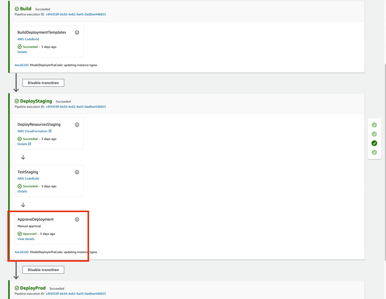
After the deployment of the endpoint, tests to check the behavior of the setup are started. For testing, Yara uses CodeBuild test reports. This feature allows developers to run unit tests, configuration tests, and functional tests pre- and post-deployment. In this case, Yara runs functional tests by passing test payloads to SageMaker endpoints and evaluating the response. After these tests are passed, the pipeline proceeds to deploy the SageMaker endpoints to TEST. The ELC backend is also deployed to TEST, which makes end-to-end testing for the app possible in this environment. Additionally, Yara runs user-acceptance testing in TEST. The trigger from TEST to PROD deployment is a manual approval action. After the new model version has passed both functional and user acceptance testing in TEST, the engineering team approves the model deployment to PROD.

The following figure illustrates this workflow.

Common components

For ELC, we use several components that are common for all deployment stages (DEV, TEST, PROD) and models. These components reside in our deployment account, and include model version control, a container image repository, an encryption key, and a bucket to store common artifacts.

There are several advantages of using common artifacts. For example, the resources don’t have to be created for every account, which enforces compatibility between the accounts. That means we build container images once and reuse them in all target accounts, reducing build time.

This pipeline stores the different model versions in a common model registry in the deployment account. From this central location, models can be deployed in all accounts without transferring them. Similarly, the use of a centrally stored encryption key makes it easier to manage the key and cross-account permissions.

One disadvantage of using common artifacts is that the onboarding step of a new use case can become more elaborate. To onboard a new use case, a new model registry must be created and if required a new container image repository. We also recommend creating a new encryption key to strictly separate resources and stored data.

Conclusion

In this post, we demonstrated how Yara used SageMaker and ADF to build a highly scalable MLOps platform. ML is a cross-functional capability, and teams deploy models to different business unit accounts. Therefore, ADF, which offers native integration with Organizations, makes it an ideal candidate to bootstrap accounts to set up CI/CD pipelines. Operationally, ADF pipelines run in the central deployment account, which makes it easy to get an overall health view of deployments. Finally, ADF uses AWS managed services like CodeBuild, CodeDeploy, CodePipeline, and CloudFormation, making it easy to configure and maintain.

SageMaker provides a broad spectrum of ML capabilities, which enables teams to focus more on solving business problems and less on building and maintaining infrastructure. Additionally, SageMaker Pipelines provides a rich set of APIs to create, update, and deploy ML workflows, making it a great fit for MLOps.

Lastly, MLOps provides the best practices to deploy and maintain ML models in production reliably and efficiently. It’s critical for teams who create and deploy ML solutions at scale to implement MLOps. In Yara’s case, MLOps significantly reduces the effort required to onboard a new plant, roll out updates to ELC, and ensure the models are monitored for quality.

For more information on how to deploy applications using ADF, see the examples.

About the authors

Shaheer Mansoor is a Data Scientist at AWS. His focus is on building machine learning platforms that can host AI solutions at scale. His interest areas are MLOps, feature stores, model hosting, and model monitoring.

Tim Becker is a Senior Data Scientist at Yara International. Within Digital Production, his focus is on process optimization of ammonia and nitric acid production. He holds a PhD in Thermodynamics and is passionate about bringing together process engineering and machine learning.

Yongyos Kaewpitakkun is a senior data scientist in the Digital Production team at Yara International. He has a PhD in AI/machine learning and many years of hands-on experience leveraging machine learning, computer vision, and natural language processing models to solve challenging business problems.

Read More

Image classification is a computer vision-based machine learning (ML) technique that allows you to classify images. Some well-known examples of image classification include classifying handwritten digits, medical image classification, and facial recognition. Image classification is a useful technique with several business applications, but building a good image classification model isn’t trivial.

Several considerations can play a role when evaluating an ML model. Beyond model accuracy, other potential metrics of importance are model training time and inference time. Given the iterative nature of ML model development, faster training times allow data scientists to quickly test various hypotheses. Faster inferencing can be critical in real-time applications.

Amazon SageMaker JumpStart provides one-click fine-tuning and deployment of a wide variety of pre-trained models across popular ML tasks, as well as a selection of end-to-end solutions that solve common business problems. These features remove the heavy lifting from each step of the ML process, making it easier to develop high-quality models and reducing time to deployment. JumpStart APIs allow you to programmatically deploy and fine-tune a vast selection of JumpStart-supported pre-trained models on your own datasets.

You can incrementally train and tune the ML models offered in JumpStart before deployment. At the time of writing, 87 deep-learning based image classification models are available in JumpStart.

But which model will give you the best results? In this post, we present a methodology to easily run multiple models and compare their outputs on three dimensions of interest: model accuracy, training time, and inference time.

Solution overview

JumpStart allows you to train, tune, and deploy models either from the JumpStart console using its UI or with its API. In this post, we use the API route, and present a notebook with various helper scripts. You can run this notebook and get results for easy comparison of these models against each other, and then pick a model that best suits your business need in terms of model accuracy, training time, and inference time.

The public dataset used in this post consists of nearly 55,000 images of diseased and healthy plant leaves collected under controlled conditions, with class labels ranging from 0–38. This dataset is divided into train and validation datasets, with approximately 44,000 under training and 11,000 images under validation. The following are a few sample images.

For this exercise, we selected models from two frameworks—PyTorch and TensorFlow—as offered by JumpStart. The following 15 model algorithms cover a wide range of popular neural network architectures from these frameworks:

• pytorch-ic-alexnet-FT
• pytorch-ic-densenet121-FT
• pytorch-ic-densenet201-FT
• pytorch-ic-googlenet-FT
• pytorch-ic-mobilenet-v2-FT
• pytorch-ic-resnet152-FT
• pytorch-ic-resnet34-FT
• tensorflow-ic-bit-s-r101x1-ilsvrc2012-classification-1-FT
• tensorflow-ic-imagenet-inception-resnet-v2-classification 4-FT
• tensorflow-ic-imagenet-inception-v3-classification-4-FT
• tensorflow-ic-imagenet-mobilenet-v2-050-224-classification-4-FT
• tensorflow-ic-imagenet-mobilenet-v2-075-224-classification-4-FT
• tensorflow-ic-imagenet-mobilenet-v2-140-224-classification-4-FT
• tensorflow-ic-imagenet-resnet-v2-152-classification-4-FT
• tensorflow-ic-tf2-preview-mobilenet-v2-classification-4-FT

We use the model tensorflow-ic-imagenet-inception-v3-classification-4-FT as a base against which results from other models are compared. This base model was picked arbitrarily.

The code used to run this comparison is available on the AWS Samples GitHub repo.

Results

In this section, we present the results from these 15 runs. For all these runs, the hyperparameters used were epochs = 5, learning rate = 0.001, batch size = 16.

Model accuracy, training time, and inference time from model tensorflow-ic-imagenet-inception-v3-classification-4-FT were taken as the base, and results from all other models are presented relative to this base model. Our intention here is not to show which model is the best but to rather show how, through the JumpStart API, you can compare results from various models and then choose a model that best fits your use case.

The following screenshot highlights the base model against which all other models were compared.

The following plot shows a detailed view of relative accuracy vs. relative training time. PyTorch models are color coded in red and TensorFlow models in blue.

The models highlighted with a green ellipse in the preceding plot seem to have a good combination of relative accuracy and low relative training time. The following table provides more details on these three models.

The following plot compares relative accuracy vs. relative inference time. PyTorch models are color coded in red and TensorFlow models in blue.

The following table provides details on the three models in the green ellipse.

The two plots clearly demonstrate that certain model algorithms performed better than others on the three dimensions that were selected. The flexibility offered through this exercise can help you pick the right algorithm, and by using the provided notebook, you can easily run this type of experiment on any of the 87 available models.

Conclusion

In this post, we showed how to use JumpStart to build high performing image classification models on multiple dimensions of interest, such as model accuracy, training time, and inference latency. We also provided the code to run this exercise on your own dataset; you can pick any models of interest from the 87 models that are presently available for image classification in the JumpStart model hub. We encourage you to give it a try today.

For more details on JumpStart, refer to SageMaker JumpStart.

About the Authors

Dr. Raju Penmatcha is an AI/ML Specialist Solutions Architect in AI Platforms at AWS. He received his PhD from Stanford University. He works closely on the low/no-code suite of services in SageMaker, which help customers easily build and deploy machine learning models and solutions. When not helping customers, he likes traveling to new places.

Dr. Ashish Khetan is a Senior Applied Scientist with Amazon SageMaker built-in algorithms and helps develop machine learning algorithms. He got his PhD from University of Illinois Urbana-Champaign. He is an active researcher in machine learning and statistical inference, and has published many papers in NeurIPS, ICML, ICLR, JMLR, ACL, and EMNLP conferences.

Read More

Organizations are using machine learning (ML) and AI services to enhance customer experience, reduce operational cost, and unlock new possibilities to improve business outcomes. Data underpins ML and AI use cases and is a strategic asset to an organization. As data is growing at an exponential rate, organizations are looking to set up an integrated, cost-effective, and performant data platform in order to preprocess data, perform feature engineering, and build, train, and operationalize ML models at scale. To achieve that, AWS offers a unified modern data platform that is powered by Amazon Simple Storage Service (Amazon S3) as the data lake with purpose-built tools and processing engines to support analytics and ML workloads. For a unified ML experience, you can use Amazon SageMaker Studio, which offers native integration with AWS Glue interactive sessions to perform feature engineering at scale with sensitive data protection. In this post, we demonstrate how to implement this solution.

Amazon SageMaker is a fully managed ML service that enables you to build, train, and deploy models at scale for a wide range of use cases. For model training, you can use any of the built-in algorithms within SageMaker to get started on training and deploying ML models quickly.

A key component of the model building and development process is feature engineering. AWS Glue is one of the recommended options to achieve feature engineering at scale. AWS Glue enables you to run data integration and transformation in a distributed fashion on a serverless Apache Spark infrastructure, and makes it easy to use the popular Spark ML library for feature engineering and model development. In addition, you can use AWS Glue for incremental data processing through job bookmarks, ingest data from over 100 sources using connectors, and run spiky or unpredictable workloads using auto scaling.

Another important requirement for ML-based applications is data security and access control. It’s common demand to have tighter control on who can access the most sensitive data as part of the feature engineering and model building process by following the principal of least privilege access. To achieve this, you can utilize the AWS Glue integration with AWS Lake Formation for increased governance and management of data lake assets. With Lake Formation, you can configure fine-grained data access control and security policies on top of your Amazon S3 data lake. The policies are defined in a central location, allowing multiple analytics and ML services, such as AWS Glue, Amazon Athena, and SageMaker, to interact with data stored in Amazon S3.

AWS Glue includes a personally identifiable information (PII) detection transform that provides the ability to detect, mask, or remove entities as required, for increased compliance and governance. With the PII transform, you can detect PII data in datasets and automatically apply fine-grained access control using Lake Formation to restrict sensitive data for different user groups.

Use case

We focus on a propensity model use case that includes a customer marketing dataset and involves two user personas: a data engineer and data scientist. The dataset contains per-customer information, including lead source, contact notes, job role, some flags, page views per visit, and more. The dataset also includes sensitive information like personal phone numbers.

The data engineer is responsible for building the end-to-end data processing pipeline, including data preparation, preprocessing, and access control. The data scientist is responsible for feature engineering, and training and deploying the ML model. Note that the data scientist is not allowed to access any PII sensitive data for feature engineering or training the ML model.

As part of this use case, the data engineer builds a data pipeline to preprocess the dataset, scans the dataset for any PII information, and restricts the access of the PII column to the data scientist user. As a result, when a data scientist uses the dataset to perform feature engineering and build ML models, they don’t have access to the PII sensitive column (phone numbers, in this case). The feature engineering process involves converting columns of type string to a format that is optimal for ML models. As an advanced use case, you can extend this access pattern to implement row-level and cell-level security using Lake Formation.

Solution overview

The solution contains the following high-level steps:

1. Set up resources with AWS CloudFormation.
2. Preprocess the dataset, including PII detection and fine-grained access control, on an AWS Glue interactive session.
3. Perform feature engineering on an AWS Glue interactive session.
4. Train and deploy an ML model using the SageMaker built-in XGBoost algorithm.
5. Evaluate the ML model.

The following diagram illustrates the solution architecture.

Prerequisites

To complete this tutorial, you must have the following prerequisites:

• Have an AWS account. If you don’t have an account, you can create one.
• Complete the initial setup of Lake Formation by creating a data lake administrator and changing the default Data Catalog settings to enable fine-grained access control with Lake Formation permissions. For more information, see Setting up AWS Lake Formation. See the following example AWS Command Line Interface (AWS CLI) command:

  $ aws lakeformation put-data-lake-settings —data-lake-settings DataLakeAdmins=[{DataLakePrincipalIdentifier=<your_IAM_ARN>}],CreateDatabaseDefaultPermissions=[],CreateTableDefaultPermissions=[]

• Create a SageMaker domain. You can use the Quick setup.

Set up resources with AWS CloudFormation

This post includes a CloudFormation template for a quick setup. You can review and customize it to suit your needs. If you prefer setting up resources on the AWS Management Console and the AWS CLI rather than AWS CloudFormation, see the instructions in the appendix at the end of this post.

The CloudFormation template generates the following resources:

• S3 buckets with a sample dataset
• An AWS Lambda function to load the dataset
• AWS Identity and Access Management (IAM) group, users, roles, and policies
• Lake Formation data lake settings and permissions
• SageMaker user profiles

To create your resources, complete the following steps:

1. Sign in to the console.
2. Choose Launch Stack:
   
3. Choose Next.
4. For DataEngineerPwd and DataScientistPwd, enter your own password for the data engineer and data scientist users.
5. For GlueDatabaseName, enter demo.
6. For GlueTableName, enter web_marketing.
7. For S3BucketNameForInput, enter blog-studio-pii-dataset-<your-aws-account-id>.
8. For S3BucketNameForOutput, enter blog-studio-output-<your-aws-account-id>.
9. For SageMakerDomainId, enter your SageMaker domain ID that you prepared in the prerequisite steps.
10. Choose Next.
11. On the next page, choose Next.
12. Review the details on the final page and select I acknowledge that AWS CloudFormation might create IAM resources.
13. Choose Create.

Stack creation can take up to 10 minutes. The stack creates IAM roles and SageMaker user profiles for two personas: data engineer and data scientist. It also creates a database demo and table web_marketing with a sample dataset.

At the time of stack creation, the data engineer persona has complete access to the table, but the data scientist persona doesn’t have any access to the table yet.

Preprocess the dataset

Let’s start preprocessing data on an AWS Glue interactive session. The data engineer persona wants to verify the data to see if there is sensitive data or not, and grant minimal access permission to the data scientist persona. You can download notebook from this location.

1. Sign in to the console using the data-engineer user.
2. On the SageMaker console, choose Users.
3. Select the data-engineer user and choose Open Studio.
4. Create a new notebook and choose SparkAnalytics 1.0 for Image and Glue PySpark for Kernel.
5. Start an interactive session with the following magic to install the newer version of Boto3 (this is required for using the create_data_cells_filter method):

   %additional_python_modules boto3==1.24.82

6. Initialize the session:

   import boto3
   import sys
   from awsglue.transforms import *
   from awsglue.utils import getResolvedOptions
   from pyspark.context import SparkContext
   from awsglue.context import GlueContext
   from awsglue.job import Job
   
   sc = SparkContext.getOrCreate()
   glueContext = GlueContext(sc)
   spark = glueContext.spark_session
   job = Job(glueContext)

7. Create an AWS Glue DynamicFrame from the newly created table, and resolve choice types based on catalog schema, because we want to use the schema defined in the catalog instead of the automatically inferred schema based on data:

   dyf_marketing = glueContext.create_dynamic_frame.from_catalog(
   database="demo",
   table_name="web_marketing"
   )
   
   dyf_marketing_resolved = dyf_marketing.resolveChoice(
   choice="match_catalog",
   database="demo",
   table_name="web_marketing"
   )
   
   dyf_marketing_resolved.printSchema()

8. Validate in the table whether there is any PII data using AWS Glue PII detection:

   from awsglueml.transforms import EntityDetector
   
   entities_filter = [
   "EMAIL",
   "CREDIT_CARD",
   "IP_ADDRESS",
   "MAC_ADDRESS",
   "PHONE_NUMBER"
   ]
   entity_detector = EntityDetector()
   classified_map = entity_detector.classify_columns(dyf_marketing_resolved, entities_filter, 1.0, 0.1)
   print(classified_map)

9. Verify whether the columns classified as PII contain sensitive data or not (if not, update classified_map to drop the non-sensitive columns):

   from pyspark.sql.functions import col
   dyf_marketing_resolved.toDF().select(*[col(c) for c in classified_map.keys()]).show()

10. Set up Lake Formation permissions using a data cell filter for automatically detected columns, and restrict the columns to the data scientist persona:

    lakeformation = boto3.client('lakeformation')
    sts = boto3.client('sts')
    
    account_id = sts.get_caller_identity().get('Account')
    
    # Create a data cell filter for excluding phone_number column
    lakeformation.create_data_cells_filter(
    TableData={
    'TableCatalogId': account_id,
    'DatabaseName': 'demo',
    'TableName': 'web_marketing',
    'Name': 'pii',
    'RowFilter': {
    'AllRowsWildcard': {}
    
    },
    'ColumnWildcard': {
    'ExcludedColumnNames': list(classified_map.keys())
    }
    }
    )
    
    # Grant permission on the data cell filter
    lakeformation.grant_permissions(
    Principal={
    'DataLakePrincipalIdentifier': f'arn:aws:iam::{account_id}:role/SageMakerStudioExecutionRole_data-scientist'
    },
    Resource={
    'DataCellsFilter': {
    'TableCatalogId': account_id,
    'DatabaseName': 'demo',
    'TableName': 'web_marketing',
    'Name': 'pii'
    }
    },
    Permissions=[
    'SELECT'
    ]
    )

11. Log in to Studio as data-scientist to see that the PII columns are not visible. You can download notebook from this location.
12. Create a new notebook and choose SparkAnalytics 1.0 for Image and Glue PySpark for Kernel:

    import boto3
    import sys
    from awsglue.transforms import *
    from awsglue.utils import getResolvedOptions
    from pyspark.context import SparkContext
    from awsglue.context import GlueContext
    from awsglue.job import Job
    
    sc = SparkContext.getOrCreate()
    glueContext = GlueContext(sc)
    spark = glueContext.spark_session
    job = Job(glueContext)
    
    dyf_marketing = glueContext.create_dynamic_frame.from_catalog(
    database="demo",
    table_name="web_marketing"
    )
    
    dyf_marketing.printSchema()

Perform feature engineering

We use the Apache Spark ML library to perform feature engineering as the data-scientist user and then write back the output to Amazon S3.

1. In the following cell, we apply features from the Apache Spark ML library:
   • StringIndexer maps a string column of labels to a column of label indexes.
   • OneHotEncoder maps a categorical feature, represented as a label index, to a binary vector with at most a single one-value that indicates the presence of a specific categorical feature. This transform is used for ML algorithms that expect continuous features.
   • VectorAssembler is a transformer that combines a given list of columns into a single vector column, which is then used in training ML models for algorithms such as logistic regression and decision trees.

   #feature engineering by using string indexer and one hot encoding from spark ML library
   from pyspark.ml.feature import StringIndexer, VectorIndexer, OneHotEncoder, VectorAssembler
   from pyspark.ml import Pipeline
   
   cols = ['lastcampaignactivity','region','viewedadvertisement','usedpromo','jobrole']
   
   int_cols = ['pageviewspervisit','totaltimeonwebsite','totalwebvisits',]
   
   indexers = [
   StringIndexer(inputCol=c, outputCol="{0}_indexed".format(c))
   for c in cols
   ]
   
   encoders = [
   OneHotEncoder(
   inputCol=indexer.getOutputCol(),
   outputCol="{0}_encoded".format(indexer.getOutputCol()))
   for indexer in indexers
   ]
   
   assembler = VectorAssembler(
   inputCols=[encoder.getOutputCol() for encoder in encoders]+int_cols,
   outputCol="features"
   )

2. The final transformed DataFrame can be created using the Pipeline library. A pipeline is specified as a sequence of stages. These stages are run in order and the input DataFrame is transformed as it passes through each stage.

   df_marketing = dyf_marketing.toDF()
   pipeline = Pipeline(stages=indexers + encoders + [assembler])
   df_tfm=pipeline.fit(df_marketing).transform(df_marketing)
   

3. Next, we split the dataset into train, validate, and test DataFrame and save it in the S3 bucket to train the ML model (provide your AWS account ID in the following code):

   from pyspark.ml.functions import vector_to_array
   
   #set s3 output location for feature engineering output
   bucket='blog-studio-output-<your-aws-account-id>'
   
   #convert sparse to dense vector
   df_tfm=df_tfm.select('converted',vector_to_array("features").alias("features_array"))
   
   #split features array into individual columns
   df_tfm=df_tfm.select([df_tfm.converted] + [df_tfm.features_array[i] for i in range(17)])
   
   #split the overall dataset into 70-20-10 training , validation and test
   (train_df, validation_df, test_df) = df_tfm.randomSplit([0.7,0.2,0.1])
   
   #write back train, validation and test datasets to S3
   train_df.write
   .option("header","false")
   .csv('s3://{}/web-marketing/processed/training/'.format(bucket))
   
   validation_df.write
   .option("header","false")
   .csv('s3://{}/web-marketing/processed/validation/'.format(bucket))
   
   test_df.write
   .option("header","false")
   .csv('s3://{}/web-marketing/processed/test/'.format(bucket))

Train and deploy an ML model

In the previous section, we completed feature engineering, which included converting string columns such as region, jobrole, and usedpromo into a format that is optimal for ML models. We also included columns such as pageviewspervisit and totalwebvisits, which will help us predict a customer’s propensity to buy a product.

We now train an ML model by reading the train and validation dataset using the SageMaker built-in XGBoost algorithm. Then we deploy the model and run an accuracy check. You can download notebook from this location.

In the following cell, we’re reading data from the second S3 bucket, which includes the output from our feature engineering operations. Then we use the built-in algorithm XGBoost to train the model.

1. Open a new notebook. Choose Data Science for Image and Python 3 for Kernel (provide your AWS account ID in the following code):

   #set s3 bucket location for training data
   import sagemaker
   import boto3
   from sagemaker import get_execution_role
   
   container = sagemaker.image_uris.retrieve(region=boto3.Session().region_name,
   framework='xgboost', version='latest')
   bucket='blog-studio-output-<your-aws-account-id>'
   prefix='web-marketing/processed'
   
   #read train and validation input datasets
   s3_input_train = sagemaker.inputs.TrainingInput(s3_data='s3://{}/{}/training/'
   .format(bucket, prefix), content_type='csv')
   s3_input_validation = sagemaker.inputs.TrainingInput(s3_data='s3://{}/{}/validation/'
   .format(bucket, prefix), content_type='csv')
   
   #train xgb model
   sess = sagemaker.Session()
   from sagemaker import get_execution_role
   
   xgb = sagemaker.estimator.Estimator(
   container,
   role=get_execution_role(),
   instance_count=1,
   instance_type='ml.m4.xlarge',
   output_path='s3://{}/{}/output'
   .format(bucket, prefix),
   sagemaker_session=sess
   )
   
   xgb.set_hyperparameters(
   max_depth=5,
   eta=0.2,
   gamma=4,
   min_child_weight=6,
   subsample=0.8,
   silent=0,
   objective='binary:logistic',
   num_round=100
   )
   
   xgb.fit({'train': s3_input_train, 'validation': s3_input_validation})

2. When training is complete, we can deploy the model using SageMaker hosting services:

   #deploy ml model
   xgb_predictor = xgb.deploy(initial_instance_count=1,
   instance_type='ml.m4.xlarge')

Evaluate the ML model

We use the test dataset to evaluate the model and delete the inference endpoint when we’re done to avoid any ongoing charges.

1. Evaluate the model with the following code:

   #create csv serialiser to run accuracy on test dataset
   xgb_predictor.serializer = sagemaker.serializers.CSVSerializer()
   
   #read test dataset
   import io
   import pandas as pd
   
   s3 = boto3.resource('s3')
   bucket_obj = s3.Bucket(bucket)
   
   test_line = []
   test_objs = bucket_obj.objects.filter(Prefix="web-marketing/processed/test")
   for obj in test_objs:
   try:
   key = obj.key
   body = obj.get()['Body'].read()
   temp = pd.read_csv(io.BytesIO(body),header=None, encoding='utf8',sep=',')
   test_line.append(temp)
   except:
   continue
   
   test_df = pd.concat(test_line)
   
   #predict results using deployed model
   import numpy as np
   def predict(data, predictor, rows=500 ):
   split_array = np.array_split(data, int(data.shape[0] / float(rows) + 1))
   predictions = ''
   for array in split_array:
   predictions = ','.join([predictions, predictor.predict(array).decode('utf-8')])
   return np.fromstring(predictions[1:], sep=',')
   
   #drop the target variable in test_df and make prediction
   predictions = predict(test_df.drop(test_df.columns[0], axis=1).to_numpy(), xgb_predictor)
   
   #calculate accuracy using sklearn library
   from sklearn.metrics import accuracy_score, confusion_matrix
   y_pred=np.round(predictions)
   y_true=test_df.iloc[:,0].values.tolist()
   print('Accuracy score: ',accuracy_score(y_true, y_pred))
   print('Confusion matrix: n',confusion_matrix(y_true, y_pred))

   The accuracy result for the sample run was 84.6 %. This could be slightly different for your run due to the random split of the dataset.

2. We can delete the inference endpoint with the following code:

   xgb_predictor.delete_endpoint(delete_endpoint_config=True)

Clean up

Now to the final step, cleaning up the resources.

1. Empty the two buckets created through the CloudFormation stack.
2. Delete the apps associated with user profiles data-scientist and data-engineer within Studio.
3. Delete the CloudFormation stack.

Conclusion

In this post, we demonstrated a solution that enables personas such as data engineers and data scientists to perform feature engineering at scale. With AWS Glue interactive sessions, you can easily achieve feature engineering at scale with automatic PII detection and fine-grained access control without needing to manage any underlying infrastructure. By using Studio as the single entry point, you can get a simplified and integrated experience to build an end-to-end ML workflow: from preparing and securing data to building, training, tuning, and deploying ML models. To learn more, visit Getting started with AWS Glue interactive sessions and Amazon SageMaker Studio.

We are very excited about this new capability and keen to see what you’re going to build with it!

Appendix: Set up resources via the console and the AWS CLI

Complete the instructions in this section to set up resources using the console and AWS CLI instead of the CloudFormation template.

Prerequisites

To complete this tutorial, you must have access to the AWS CLI (see Getting started with the AWS CLI) or use command line access from AWS CloudShell.

Configure IAM group, users, roles, and policies

In this section, we create two IAM users: data-engineer and data-scientist, which belong to the IAM group data-platform-group. Then we add a single IAM policy to the IAM group.

1. On the IAM console, create a policy on the JSON tab to create a new IAM managed policy named DataPlatformGroupPolicy. The policy allows users in the group to access Studio, but only using a SageMaker user profile with a tag that matches their IAM user name. Use the following JSON policy document to provide permissions:

   {
      "Version":"2012-10-17",
      "Statement":[
         {
            "Action":[
               "sagemaker:DescribeDomain",
               "sagemaker:ListDomains",
               "sagemaker:ListUserProfiles",
               "sagemaker:ListApps"
            ],
            "Resource":"*",
            "Effect":"Allow",
            "Sid":"AmazonSageMakerStudioReadOnly"
         },
         {
            "Action":"sagemaker:AddTags",
            "Resource":"*",
            "Effect":"Allow",
            "Sid":"AmazonSageMakerAddTags"
         },
         {
            "Condition":{
               "StringEquals":{
                  "sagemaker:ResourceTag/studiouserid":"${aws:username}"
               }
            },
            "Action":[
               "sagemaker:CreatePresignedDomainUrl",
               "sagemaker:DescribeUserProfile"
            ],
            "Resource":"*",
            "Effect":"Allow",
            "Sid":"AmazonSageMakerAllowedUserProfile"
         },
         {
            "Condition":{
               "StringNotEquals":{
                  "sagemaker:ResourceTag/studiouserid":"${aws:username}"
               }
            },
            "Action":[
               "sagemaker:CreatePresignedDomainUrl",
               "sagemaker:DescribeUserProfile"
            ],
            "Resource":"*",
            "Effect":"Deny",
            "Sid":"AmazonSageMakerDeniedUserProfiles"
         }
      ]
   }

2. Create an IAM group called data-platform-group.
3. Search and attach the AWS managed policy named DataPlatformGroupPolicy to the group.
4. Create IAM users called data-engineer and data-scientist under the IAM group data-platform-group.
5. Create a new managed policy named SageMakerExecutionPolicy (provide your Region and account ID in the following code):

   {
      "Version":"2012-10-17",
      "Statement":[
         {
            "Action":[
               "sagemaker:DescribeDomain",
               "sagemaker:ListDomains",
               "sagemaker:ListUserProfiles",
               "sagemaker:ListApps"
            ],
            "Resource":"*",
            "Effect":"Allow",
            "Sid":"AmazonSageMakerStudioReadOnly"
         },
         {
            "Action":"sagemaker:AddTags",
            "Resource":"*",
            "Effect":"Allow",
            "Sid":"AmazonSageMakerAddTags"
         },
         {
            "Action":[
               "sagemaker:CreateTrainingJob",
               "sagemaker:DescribeTrainingJob",
               "logs:DescribeLogStreams",
               "sagemaker:CreateModel",
               "sagemaker:CreateEndpointConfig",
               "sagemaker:CreateEndpoint",
               "sagemaker:DescribeEndpoint",
               "sagemaker:InvokeEndpoint",
               "sagemaker:DeleteEndpointConfig",
               "sagemaker:DeleteEndpoint"
            ],
            "Resource":"*",
            "Effect":"Allow",
            "Sid":"AmazonSageMakerTrainingAndDeploy"
         },
         {
            "Action":"sagemaker:*App",
            "Resource":"arn:aws:sagemaker:<aws region>:<account id>:app/*/${aws:PrincipalTag/userprofilename}/*",
            "Effect":"Allow",
            "Sid":"AmazonSageMakerAllowedApp"
         },
         {
            "Action":"sagemaker:*App",
            "Effect":"Deny",
            "NotResource":"arn:aws:sagemaker:<aws region>:<account id>:app/*/${aws:PrincipalTag/userprofilename}/*",
            "Sid":"AmazonSageMakerDeniedApps"
         },
         {
            "Action":[
               "glue:GetTable",
               "glue:GetTables",
               "glue:SearchTables",
               "glue:GetDatabase",
               "glue:GetDatabases",
               "glue:GetPartition",
               "glue:GetPartitions"
            ],
            "Resource":[
               "arn:aws:glue:<aws region>:<account id>:table/demo/*",
               "arn:aws:glue:<aws region>:<account id>:database/demo",
               "arn:aws:glue:<aws region>:<account id>:catalog"
            ],
            "Effect":"Allow",
            "Sid":"GlueCatalogPermissions"
         },
         {
            "Action":[
               "lakeformation:GetDataAccess",
               "lakeformation:StartQueryPlanning",
               "lakeformation:GetQueryState",
               "lakeformation:GetWorkUnits",
               "lakeformation:GetWorkUnitResults"
            ],
            "Resource":"*",
            "Effect":"Allow",
            "Sid":"LakeFormationPermissions"
         },
         {
            "Effect":"Allow",
            "Action":[
               "s3:CreateBucket",
               "s3:GetObject",
               "s3:PutObject",
               "s3:ListBucket",
               "s3:DeleteObject"
            ],
            "Resource":[
               "arn:aws:s3:::blog-studio-output-<account id>",
               "arn:aws:s3:::blog-studio-output-<account id>/*"
            ]
         },
         {
            "Action":[
               "iam:PassRole",
               "iam:GetRole",
               "sts:GetCallerIdentity"
            ],
            "Resource":"*",
            "Effect":"Allow",
            "Sid":"AmazonSageMakerStudioIAMPassRole"
         },
         {
            "Action":"sts:AssumeRole",
            "Resource":"*",
            "Effect":"Deny",
            "Sid":"DenyAssummingOtherIAMRoles"
         }
      ]
   }

6. Create a new managed policy named SageMakerAdminPolicy:

   {
      "Version":"2012-10-17",
      "Statement":[
         {
            "Action":[
               "lakeformation:GrantPermissions",
               "lakeformation:RevokePermissions",
               "lakeformation:ListPermissions",
               "lakeformation:BatchGrantPermissions",
               "lakeformation:BatchRevokePermissions",
               "lakeformation:CreateDataCellsFilter",
               "lakeformation:DeleteDataCellsFilter",
               "lakeformation:ListDataCellsFilter",
               "glue:GetUserDefinedFunctions",
               "glue:BatchGetCustomEntityTypes"
            ],
            "Resource":"*",
            "Effect":"Allow",
            "Sid":"GlueLakeFormationPermissions"
         }
      ]
   }

7. Create an IAM role for SageMaker for the data engineer (data-engineer), which is used as the corresponding user profile’s execution role. On the Attach permissions policy page, AmazonSageMakerFullAccess (AWS managed policy) is attached by default. You remove this policy later to maintain minimum privilege.
   1. For Role name, use the naming convention introduced at the beginning of this section to name the role SageMakerStudioExecutionRole_data-engineer.
   2. For Tags, add the key userprofilename and the value data-engineer.
   3. Choose Create role.
   4. To add the remaining policies, on the Roles page, choose the role name you just created.
   5. Under Permissions, remove the policy AmazonSageMakerFullAccess.
   6. On the Attach permissions policy page, select the AWS managed policy AwsGlueSessionUserRestrictedServiceRole, and the customer managed policies SageMakerExecutionPolicy and SageMakerAdminPolicy that you created.
   7. Choose Attach policies.
   8. Modify your role’s trust relationship:

   {
      "Version":"2012-10-17",
      "Statement":[
         {
            "Effect":"Allow",
            "Principal":{
               "Service":[
                  "glue.amazonaws.com",
                  "sagemaker.amazonaws.com"
               ]
            },
            "Action":"sts:AssumeRole"
         }
      ]
   }

8. Create an IAM role for SageMaker for the data scientist (data-scientist), which is used as the corresponding user profile’s execution role.
   1. For Role name, name the role SageMakerStudioExecutionRole_data-scientist.
   2. For Tags, add the key userprofilename and the value data-scientist.
   3. Choose Create role.
   4. To add the remaining policies, on the Roles page, choose the role name you just created.
   5. Under Permissions, remove the policy AmazonSageMakerFullAccess.
   6. On the Attach permissions policy page, select the AWS managed policy AwsGlueSessionUserRestrictedServiceRole, and the customer managed policy SageMakerExecutionPolicy that you created.
   7. Choose Attach policies.
   8. Modify your role’s trust relationship:

   {
      "Version":"2012-10-17",
      "Statement":[
         {
            "Effect":"Allow",
            "Principal":{
               "Service":[
                  "glue.amazonaws.com",
                  "sagemaker.amazonaws.com"
               ]
            },
            "Action":"sts:AssumeRole"
         }
      ]
   }

Configure SageMaker user profiles

To create your SageMaker user profiles with the studiouserid tag, complete the following steps:

1. Use the AWS CLI or CloudShell to create the Studio user profile for the data engineer (provide your account ID and Studio domain ID in the following code):

   aws sagemaker create-user-profile --domain-id <domain id> --user-profile-name data-engineer --tags Key=studiouserid,Value=data-engineer --user-settings ExecutionRole=arn:aws:iam::<account id>:role/SageMakerStudioExecutionRole_data-engineer

2. Repeat the step to create a user profile for the data scientist, replacing the account ID and Studio domain ID:

   aws sagemaker create-user-profile --domain-id <domain id> --user-profile-name data-scientist --tags Key=studiouserid,Value=data-scientist --user-settings ExecutionRole=arn:aws:iam::<account id>:role/SageMakerStudioExecutionRole_data-scientist

Create S3 buckets and upload the sample dataset

In this section, you create two S3 buckets. The first bucket has a sample dataset related to web marketing. The second bucket is used by the data scientist to store output from feature engineering tasks, and this output dataset is used to train the ML model.

First, create the S3 bucket for the input data:

1. Download the dataset.
2. On the Amazon S3 console, choose Buckets in the navigation pane.
3. Choose Create bucket.
4. For Region, choose the Region with the SageMaker domain that includes the user profiles you created.
5. For Bucket name, enter blog-studio-pii-dataset-<your-aws-account-id>.
6. Choose Create bucket.
7. Select the bucket you created and choose Upload.
8. In the Select files section, choose Add files and upload the dataset you downloaded.
   Now you create the bucket for the output data:
9. On the Buckets page, choose Create bucket.
10. For Region, choose the Region with the SageMaker domain that includes the user profiles you created.
11. For Bucket name, enter blog-studio-output-<your-aws-account-id>.
12. Choose Create bucket.

Create an AWS Glue database and table

In this section, you create an AWS Glue database and table for the dataset.

1. On the Lake Formation console, under Data catalog in the navigation pane, choose Databases.
2. Choose Add database.
3. For Name, enter demo.
4. Choose Create database.
5. Under Data catalog, choose Tables.
6. For Name, enter web_marketing.
7. For Database, select demo.
8. For Include path, enter the path of your S3 bucket for input data.
9. For Classification, choose CSV.
10. Under Schema, choose Upload Schema.
11. Enter the following JSON array into the text box:

    [
       {
          "Name":"lastcampaignactivity",
          "Type":"string"
       },
       {
          "Name":"pageviewspervisit",
          "Type":"double"
       },
       {
          "Name":"totaltimeonwebsite",
          "Type":"bigint"
       },
       {
          "Name":"totalwebvisits",
          "Type":"bigint"
       },
       {
          "Name":"attendedmarketingevent",
          "Type":"string"
       },
       {
          "Name":"organicsearch",
          "Type":"string"
       },
       {
          "Name":"viewedadvertisement",
          "Type":"string"
       },
       {
          "Name":"leadsource",
          "Type":"string"
       },
       {
          "Name":"jobrole",
          "Type":"string"
       },
       {
          "Name":"contactnotes",
          "Type":"string"
       },
       {
          "Name":"leadprofile",
          "Type":"string"
       },
       {
          "Name":"usedpromo",
          "Type":"string"
       },
       {
          "Name":"donotreachout",
          "Type":"boolean"
       },
       {
          "Name":"city",
          "Type":"string"
       },
       {
          "Name":"converted",
          "Type":"bigint"
       },
       {
          "Name":"region",
          "Type":"string"
       },
       {
          "Name":"phone_number",
          "Type":"string"
       }
    ]

12. Choose Upload.
13. Choose Submit.
14. Under Table details, choose Edit table.
15. Under Table properties, choose Add.
16. For Key, enter skip.header.line.count, and for Value, enter 1.
17. Choose Save.

Configure Lake Formation permissions

In this section, you set up Lake Formation permissions to allow IAM role SageMakerStudioExecutionRole_data-engineer to create a database and register the S3 location within Lake Formation.

First, register the data lake location to manage tables under the location in Lake Formation permissions:

1. Choose Data lake locations.
2. Choose Register location.
3. For Amazon S3 path, enter s3://blog-studio-pii-dataset-<your-aws-account-id>/ (the bucket that contains the dataset).
4. Choose Register location.
   Now you grant Lake Formation database and table permissions to the IAM roles SageMakerStudioExecutionRole_data-engineer and SageMakerStudioExecutionRole_data-scientist.First, grant database permission for SageMakerStudioExecutionRole_data-engineer:
5. Under Permissions, choose Data lake permissions.
6. Under Data permission, choose Grant.
7. For Principals, choose IAM users and roles, and select the role SageMakerStudioExecutionRole_data-engineer.
8. For Policy tags or catalog resources, choose Named data catalog resources.
9. For Databases, choose demo.
10. For Database permissions, select Super.
11. Choose Grant.
    Next, grant table permission for SageMakerStudioExecutionRole_data-engineer:
12. Under Data permission, choose Grant.
13. For Principals, choose IAM users and roles, and select the role SageMakerStudioExecutionRole_data-engineer.
14. For Policy tags or catalog resources, choose Named data catalog resources.
15. For Databases, choose demo.
16. For Tables, choose web_marketing.
17. For Table permissions, select Super.
18. For Grantable permissions, select Super.
19. Choose Grant.
    Finally, grant database permission for SageMakerStudioExecutionRole_data-scientist:
20. Under Data permission, choose Grant.
21. For Principals, choose IAM users and roles, and select the role SageMakerStudioExecutionRole_data-scientist.
22. For Policy tags or catalog resources, choose Named data catalog resources.
23. For Databases, choose demo.
24. For Database permissions, select Describe.
25. Choose Grant.

About the Authors

Praveen Kumar is an Analytics Solution Architect at AWS with expertise in designing, building, and implementing modern data and analytics platforms using cloud-native services. His areas of interests are serverless technology, modern cloud data warehouses, streaming, and ML applications.

Noritaka Sekiyama is a Principal Big Data Architect on the AWS Glue team. He enjoys collaborating with different teams to deliver results like this post. In his spare time, he enjoys playing video games with his family.

Read More

A well-designed CI/CD pipeline is essential to scale any software development workflow effectively. When designing production CI/CD pipelines, AWS recommends leveraging multiple accounts to isolate resources, contain security threats and simplify billing-and data science pipelines are no different. At AWS, we’re continuing to innovate to simplify the MLOps workflow.

In this post, we discuss some of the newer cross-account features to Amazon SageMaker that allow you to better share and manage model groups as well as manage model versions. For an example account structure to follow organizational unit best practices to host models using SageMaker endpoints across accounts, refer to MLOps Workload Orchestrator.

Solution overview

The following diagram illustrates our shared model registry architecture.

Some things to note in the preceding architecture:

• Accounts follow a principle of least privilege to follow security best practices
• The model and container registry are centralized in a shared services account
• Amazon Elastic Container Registry (Amazon ECR) is optional; it’s only required if your model requires its own environment

The following steps correspond to the diagram:

1. A data scientist registers a model from the data science account into the shared services SageMaker model registry in a PendingManualApproval state. The model artifact is created in the shared services account Amazon Simple Storage Service (Amazon S3) bucket.
2. Upon a new model version registration, someone with the authority to approve the model based on the metrics should approve or reject the model.
3. After the model is approved, the CI/CD pipeline in deployment account is triggered to deploy the updated model details in the QA account and update the stage as QA.
4. Upon passing the testing process, you can either choose to have a manual approval step within your CI/CD process or have your CI/CD pipeline directly deploy the model to production and update the stage as Prod.
5. The production environment references the approved model and code, perhaps doing an A/B test in production. In case of an audit or any issue with the model, you can use Amazon SageMaker ML Lineage Tracking. It creates and stores information about the steps of a machine learning (ML) workflow from data preparation to model deployment. With the tracking information, you can reproduce the workflow steps, track the model and dataset lineage, and establish model governance and audit standards.

Throughout the whole process, the shared model registry retains the older model versions. This allows the team to roll back changes, or even host production variants.

Prerequisites

Make sure you have the following prerequisites:

• A provisioned multi-account structure – For instructions, see Best Practices for Organizational Units with AWS Organizations. For the purposes of this blog we are leveraging the following accounts:
  • Data science account – An account where data scientists have access to the training data and create the models.
  • Shared services account – A central account for storing the model artifacts (as shown in the architecture diagram) to be accessed across the different workload accounts.
  • Deployment account – An account responsible for deploying changes to the various accounts.
  • Workload accounts – These are commonly QA and prod environments where software engineers are able to build applications to consume the ML model.
• A deployment account with appropriate permissions – For more information about best practices with a multi-account OU structure, refer to Deployments OU. This account is responsible for pointing the workload accounts to the desired model in the shared services account’s model registry.

Define cross-account policies

In following the principle of least privilege, first we need to add cross-account resource policies to the shared services resources to grant access from the other accounts.

Because the model artifacts are stored in the shared services account’s S3 bucket, the data science account needs Amazon S3 read/write access to push trained models to Amazon S3. The following code illustrates this policy, but don’t add it to the shared services account yet:

#Data Science account's policy to access Shared Services' S3 bucket
 {
    'Version': '2012-10-17',
    'Statement': [{
        'Sid': 'AddPerm',
        'Effect': 'Allow',
        'Principal': {
            'AWS': 'arn:aws:iam::<data_science_account_id>:root'
        }, 
        "Action": [ 
            's3:PutObject', 
            's3:PutObjectAcl',
            's3:GetObject', 
            's3:GetObjectVersion'
        ], #read/write
        'Resource': 'arn:aws:s3:::<shared_bucket>/*'
    }]
}

The deployment account only needs to be granted read access to the S3 bucket, so that it can use the model artifacts to deploy to SageMaker endpoints. We also need to attach the following policy to the shared services S3 bucket:

#Deployment account's policy to access Shared Services' S3 bucket
 {
    'Version': '2012-10-17',
    'Statement': [{
        'Sid': 'AddPerm',
        'Effect': 'Allow',
        'Principal': {
            'AWS': 'arn:aws:iam::<deployment_account_id>:root'
        },
        'Action': [ 
            's3:GetObject', 
            's3:GetObjectVersion'
        ], #read
        'Resource': 'arn:aws:s3:::<shared_bucket>/*'
    }]
}

We combine both policies to get the following final policy. Create this policy in the shared services account after replacing the appropriate account IDs:

{
  "Version": "2012-10-17",
  "Statement": [{
    "Sid": "AddPerm",
    "Effect": "Allow",
    "Principal": {
      "AWS": "arn:aws:iam::<data_science_account_id>:root"    
    },
    "Action": [
      "s3:PutObject",
      "s3:PutObjectAcl",
      "s3:GetObject",
      "s3:GetObjectVersion"    ],
    "Resource": "arn:aws:s3:::<shared_bucket>/*"  
    },
    {
      "Sid": "AddPermDeployment",
      "Effect": "Allow",
      "Principal": {
        "AWS": "arn:aws:iam::<deployment_account_id>:root"      
      },
      "Action": [
        "s3:GetObject",
        "s3:GetObjectVersion"      ], 
      "Resource": "arn:aws:s3:::<shared_bucket>/*"    
    }
  ]
}

To be able to deploy a model created in a different account, the user must have a role that has access to SageMaker actions, such as a role with the AmazonSageMakerFullAccess managed policy. Refer to Deploy a Model Version from a Different Account for additional details.

We need to define the model group that contains the model versions we want to deploy. Also, we want to grant permissions to the data science account. This can be accomplished in the following steps. We refer to the accounts as follows:

• shared_services_account_id – The account where the model registry is and where we want the model to be
• data_science_account_id – The account where we will be training and therefore creating the actual model artifact
• deployment_account_id – The account where we want to host the endpoint for this model

First we need to ensure the model package groups exists. You can use Boto3 APIs as shown the following example, or you can use the AWS Management Console to create the model package. Refer to Create Model Package Group for more details. This assumes you have the Boto3 installed.

model_package_group_name = "cross-account-example-model"
sm_client = boto3.Session().client("sagemaker")

create_model_package_group_response = sm_client.create_model_package_group(
    ModelPackageGroupName=model_package_group_name,
    ModelPackageGroupDescription="Cross account model package group",
    Tags=[
          {
              'Key': 'Name',
              'Value': 'cross_account_test'
          },
      ]

)

print('ModelPackageGroup Arn : {}'.format(create_model_package_group_response['ModelPackageGroupArn']))

For the permissions for this model package group, you can create a JSON document resembling the following code. Replace the actual account IDs and model package group name with your own values.

{
  "Version": "2012-10-17",
  "Statement": [
    {
      "Sid": "AddPermModelPackageGroupCrossAccount",
      "Effect": "Allow",
      "Principal": {
        "AWS": "arn:aws:iam::<data_science_account_id>:root"      
      },
      "Action": [
        "sagemaker:DescribeModelPackageGroup"      
        ],
      "Resource": "arn:aws:sagemaker:<region>:<shared_services_account_id>:model-package-group/<model_package_group_name>"    
    },
    {
      "Sid": "AddPermModelPackageVersionCrossAccount",
      "Effect": "Allow",
      "Principal": {
        "AWS": "arn:aws:iam::<data_science_account_id>:root"      
      },
      "Action": [
        "sagemaker:DescribeModelPackage",
        "sagemaker:ListModelPackages",
        "sagemaker:UpdateModelPackage",
        "sagemaker:CreateModelPackage",
        "sagemaker:CreateModel"      
      ],
      "Resource": "arn:aws:sagemaker:<region>:<shared_services_account_id>:model-package/<model_package_group_name>/*"    
    }
  ]
}

Finally, apply the policy to the model package group. You can’t associate this policy with the package group via the console. You need the SDK or AWS Command Line Interface (AWS CLI) access. For example, the following code uses Boto3:

# Convert the policy from JSON dict to string
model_package_group_policy = dict(<put-above-json-policy-after-subsitute> )
model_package_group_policy = json.dumps(model_package_group_policy)

# Set the new policy
sm_client = boto3.Session().client("sagemaker")
response = sm_client.put_model_package_group_policy(
    ModelPackageGroupName = model_package_group_name,
    ResourcePolicy = model_package_group_policy)

We also need a custom AWS Key Management Service (AWS KMS) key to encrypt the model while storing it in Amazon S3. This needs to be done using the data science account. On the AWS KMS console, navigate to the Define key usage permissions page. In the Other AWS accounts section, choose Add another AWS account. Enter the AWS account number for the deployment account. You use this KMS key for the SageMaker training job. If you don’t specify a KMS key for the training job, SageMaker defaults to an Amazon S3 server-side encryption key. A default Amazon S3 server-side encryption key can’t be shared with or used by another AWS account.

The policy and permissions follow this pattern:

• The Amazon S3 policy specified in shared_services_account gives permissions to the data science account and deployments account
• The KMS key policy specified in shared_services_account gives permissions to the data science account and deployments account

We need to ensure that the shared services account and deployment account have access to the Docker images that were used for training the model. These images are generally hosted in AWS accounts, and your account admin can help you get access, if you don’t have access already. For this post, we don’t create any custom Docker images after training the model and therefore we don’t need any specific Amazon ECR policies for the images.

In the workload accounts (QA or prod), we need to create two AWS Identity and Access Management (IAM) policies similar to the following. These are inline policies, which means that they’re embedded in an IAM identity. This gives these accounts access to model registry.

The first inline policy allows a role to access the Amazon S3 resource in the shared services account that contains the model artifact. Provide the name of the S3 bucket and your model:

{
    "Version": "2012-10-17",
    "Statement": [
        {
            "Effect": "Allow",
            "Action": "s3:GetObject",
            "Resource": "arn:aws:s3:::<bucket-name>/sagemaker/<cross-account-example-model>/output/model.tar.gz"
        }
    ]
}

The second inline policy allows a role, which we create later, to use the KMS key in the shared services account. Specify the account ID for the shared services account and KMS key ID:

{
    "Version": "2012-10-17",
    "Statement": [
        {
            "Sid": "AllowUseOfTheKey",
            "Effect": "Allow",
            "Action": [
                "kms:Decrypt"
            ],
            "Resource": [
                "arn:aws:kms:us-east-1:<data_science_account_id>:key/{xxxxxxxx-xxxx-xxxx-xxxx-xxxxxxxxxxxx}"
            ]
        }
    ]
}

Finally, we need to create an IAM role for SageMaker. This role has the AmazonSageMakerFullAccess policy attached. We then attach these two inline policies to the role we created. If you’re using an existing SageMaker execution role, attach these two policies to that role. For instructions, refer to Creating roles and attaching policies (console).

Now that we have defined the policies of each account, let’s use an example to see it in action.

Build and train a model using a SageMaker pipeline

We first create a SageMaker pipeline in the data science account for carrying out data processing, model training, and evaluation. We use the California housing dataset obtained from the StatLib library. In the following code snippet, we use a custom preprocessing script preprocess.py to perform some simple feature transformation such as feature scaling, which can be generated using the following notebook. This script also splits the dataset into training and test datasets.

We create a SKLearnProcessor object to run this preprocessing script. In the SageMaker pipeline, we create a processing step (ProcessingStep) to run the processing code using SKLearnProcessor. This processing code is called when the SageMaker pipeline is initialized. The code creating the SKLearnProcessor and ProcessingStep are shown in the following code. Note that all the code in this section is run in the data science account.

# Useful SageMaker variables - Create a Pipeline session which will lazy init resources
session = PipelineSession()

framework_version = "0.23-1"

# Create SKlearn processor object,
# The object contains information about what instance type to use, the IAM role to use etc.
# A managed processor comes with a preconfigured container, so only specifying version is required.
sklearn_processor = SKLearnProcessor(
    framework_version=framework_version,
    role=role,
    instance_type=processing_instance_type,
    instance_count=1,
    base_job_name="tf2-california-housing-processing-job",
    sagemaker_session=session
)

# Use the sklearn_processor in a SageMaker pipelines ProcessingStep
step_preprocess_data = ProcessingStep(
    name="Preprocess-California-Housing-Data",
    processor=sklearn_processor,
    inputs=[
        ProcessingInput(source=input_data, destination="/opt/ml/processing/input"),
    ],
    outputs=[
        ProcessingOutput(output_name="train", source="/opt/ml/processing/train"),
        ProcessingOutput(output_name="test", source="/opt/ml/processing/test"),
    ],
    code="preprocess.py",
)

We need a custom KMS key to encrypt the model while storing it to Amazon S3. See the following code:

kms_client = boto3.client('kms')
response = kms_client.describe_key(
    KeyId='alias/sagemaker/outkey',
)
key_id = response['KeyMetadata']['KeyId']

To train the model, we create a TensorFlow estimator object. We pass it the KMS key ID along with our training script train.py, training instance type, and count. We also create a TrainingStep to be added to our pipeline, and add the TensorFlow estimator to it. See the following code:

model_path = f"s3://{bucket}/{prefix}/model/"

hyperparameters = {"epochs": training_epochs}
tensorflow_version = "2.4.1"
python_version = "py37"

tf2_estimator = TensorFlow(
    source_dir="code",
    entry_point="train.py",
    instance_type=training_instance_type,
    instance_count=1,
    framework_version=tensorflow_version,
    role=role,
    base_job_name="tf2-california-housing-train",
    output_path=model_path,
    output_kms_key=key_id,
    hyperparameters=hyperparameters,
    py_version=python_version,
    sagemaker_session=session
)

# Use the tf2_estimator in a SageMaker pipelines ProcessingStep.
# NOTE how the input to the training job directly references the output of the previous step.
step_train_model = TrainingStep(
    name="Train-California-Housing-Model",
    estimator=tf2_estimator,
    inputs={
        "train": TrainingInput(
            s3_data=step_preprocess_data.properties.ProcessingOutputConfig.Outputs[
                "train"
            ].S3Output.S3Uri,
            content_type="text/csv",
        ),
        "test": TrainingInput(
            s3_data=step_preprocess_data.properties.ProcessingOutputConfig.Outputs[
                "test"
            ].S3Output.S3Uri,
            content_type="text/csv",
        ),
    },
)

In addition to training, we need to carry out model evaluation, for which we use mean squared error (MSE) as the metric in this example. The earlier notebook also generates evaluate.py, which we use to evaluate our a model using MSE. We also create a ProcessingStep to initialize the model evaluation script using a SKLearnProcessor object. The following code creates this step:

from sagemaker.workflow.properties import PropertyFile

# Create SKLearnProcessor object.
# The object contains information about what container to use, what instance type etc.
evaluate_model_processor = SKLearnProcessor(
    framework_version=framework_version,
    instance_type=processing_instance_type,
    instance_count=1,
    base_job_name="tf2-california-housing-evaluate",
    role=role,
    sagemaker_session=session
)

# Create a PropertyFile
# A PropertyFile is used to be able to reference outputs from a processing step, for instance to use in a condition step.
# For more information, visit https://docs.aws.amazon.com/sagemaker/latest/dg/build-and-manage-propertyfile.html
evaluation_report = PropertyFile(
    name="EvaluationReport", output_name="evaluation", path="evaluation.json"
)

# Use the evaluate_model_processor in a SageMaker pipelines ProcessingStep.
step_evaluate_model = ProcessingStep(
    name="Evaluate-California-Housing-Model",
    processor=evaluate_model_processor,
    inputs=[
        ProcessingInput(
            source=step_train_model.properties.ModelArtifacts.S3ModelArtifacts,
            destination="/opt/ml/processing/model",
        ),
        ProcessingInput(
            source=step_preprocess_data.properties.ProcessingOutputConfig.Outputs[
                "test"
            ].S3Output.S3Uri,
            destination="/opt/ml/processing/test",
        ),
    ],
    outputs=[
        ProcessingOutput(output_name="evaluation", source="/opt/ml/processing/evaluation"),
    ],
    code="evaluate.py",
    property_files=[evaluation_report],
)

After model evaluation, we also need a step to register our model with the model registry, if the model performance meets the requirements. This is shown in the following code using the RegisterModel step. Here we need to specify the model package that we had declared in the shared services account. Replace the Region, account, and model package with your values. The model name used here is modeltest, but you can use any name of your choice.

# Create ModelMetrics object using the evaluation report from the evaluation step
# A ModelMetrics object contains metrics captured from a model.
model_metrics = ModelMetrics(
    model_statistics=MetricsSource(
        s3_uri=evaluation_s3_uri,
        content_type="application/json",
    )
)

# Create a RegisterModel step, which registers the model with SageMaker Model Registry.
model = Model(
    image_uri=tf2_estimator.training_image_uri(),
    model_data=training_step.properties.ModelArtifacts.S3ModelArtifacts,
    source_dir=tf2_estimator.source_dir,
    entry_point=tf2_estimator.entry_point,
    role=role_arn,
    sagemaker_session=session
)

model_registry_args = model.register(
    content_types=['text/csv'],
    response_types=['application/json'],
    inference_instances=['ml.t2.medium', 'ml.m5.xlarge'],
    transform_instances=['ml.m5.xlarge'],
    model_package_group_name=model_package_group_name,
    approval_status='PendingManualApproval',
    model_metrics=model_metrics
)

 step_register_model= ModelStep(
    name='RegisterModel',
    step_args=model_registry_args
)

We also need to create the model artifacts so that it can be deployed (using the other account). For creating the model, we create a CreateModelStep, as shown in the following code:

from sagemaker.inputs import CreateModelInput 
from sagemaker.workflow.model_step import ModelStep 
step_create_model = ModelStep( 
    name="Create-California-Housing-Model", 
    step_args=model.create(instance_type="ml.m5.large",accelerator_type="ml.eia1.medium"),
 )

Adding conditions to the pipeline is done with a ConditionStep. In this case, we only want to register the new model version with the model registry if the new model meets an accuracy condition. See the following code:

from sagemaker.workflow.conditions import ConditionLessThanOrEqualTo
from sagemaker.workflow.condition_step import (
    ConditionStep,
    JsonGet,
)

# Create accuracy condition to ensure the model meets performance requirements.
# Models with a test accuracy lower than the condition will not be registered with the model registry.
cond_lte = ConditionLessThanOrEqualTo(
    left=JsonGet(
        step=step_evaluate_model,
        property_file=evaluation_report,
        json_path="regression_metrics.mse.value",
    ),
    right=accuracy_mse_threshold,
)

# Create a SageMaker Pipelines ConditionStep, using the preceding condition.
# Enter the steps to perform if the condition returns True / False.
step_cond = ConditionStep(
    name="MSE-Lower-Than-Threshold-Condition",
    conditions=[cond_lte],
    if_steps=[step_register_model, step_create_model],
    else_steps=[step_higher_mse_send_email_lambda],
)

Finally, we want to orchestrate all the pipeline steps so that the pipeline can be initialized:

from sagemaker.workflow.pipeline import Pipeline

# Create a SageMaker Pipeline.
# Each parameter for the pipeline must be set as a parameter explicitly when the pipeline is created.
# Also pass in each of the preceding steps.
# Note that the order of execution is determined from each step's dependencies on other steps,
# not on the order they are passed in.
pipeline = Pipeline(
    name=pipeline_name,
    parameters=[
        processing_instance_type,
        training_instance_type,
        input_data,
        training_epochs,
        accuracy_mse_threshold,
        endpoint_instance_type,
    ],
    steps=[step_preprocess_data, step_train_model, step_evaluate_model, step_cond],
)

Deploy a model version from a different account

Now that the model has been registered in the shared services account, we need to deploy into our workload accounts using the CI/CD pipeline in the deployment account. We have already configured the role and the policy in an earlier step. We use the model package ARN to deploy the model from the model registry. The following code runs in the deployment account and is used to deploy approved models to QA and prod:

from sagemaker import ModelPackage
from time import gmtime, strftime

sagemaker_session = sagemaker.Session(boto_session=sess)

model_package_arn = 'arn:aws:sagemaker:<region>:<shared_services_account>:<model_group_package>/modeltest/version_number'
model = ModelPackage(role=role, 
                     model_package_arn=model_package_arn, 
                     sagemaker_session=sagemaker_session)
model.deploy(initial_instance_count=1, instance_type='ml.m5.xlarge')

Conclusion

In this post, we demonstrated how to set up the policies needed for a multi-account setup for ML based on the principle of least privilege. Then we showed the process of building and training the models in the data science account. Finally, we used the CI/CD pipeline in the deployment account to deploy the latest version of approved models to QA and production accounts. Additionally, you can view the deployment history of models and build triggers in AWS CodeBuild.

You can scale the concepts in this post to host models in Amazon Elastic Compute Cloud (Amazon EC2) or Amazon Elastic Kubernetes Service (Amazon EKS), as well as build out a batch inference pipeline.

To learn more about having separate accounts that build ML models in AWS, see Best Practices for Organizational Units with AWS Organizations and Safely update models in production.

About the Authors

Sandeep Verma is a Sr. Prototyping Architect with AWS. He enjoys diving deep into customer challenges and building prototypes for customers to accelerate innovation. He has a background in AI/ML, founder of New Knowledge, and generally passionate about tech. In his free time, he loves traveling and skiing with his family.

 Mani Khanuja is an Artificial Intelligence and Machine Learning Specialist SA at Amazon Web Services (AWS). She helps customers using machine learning to solve their business challenges using the AWS. She spends most of her time diving deep and teaching customers on AI/ML projects related to computer vision, natural language processing, forecasting, ML at the edge, and more. She is passionate about ML at edge, therefore, she has created her own lab with self-driving kit and prototype manufacturing production line, where she spend lot of her free time.

Saumitra Vikram is a Software Developer on the Amazon SageMaker team and is based in Chennai, India. Outside of work, he loves spending time running, trekking and motor bike riding through the Himalayas.

Sreedevi Srinivasan is an engineering leader in AWS SageMaker. She is passionate and excited about enabling ML as a platform that is set to transform every day lives. She currently focusses on SageMaker Feature Store. In her free time, she likes to spend time with her family.

Rupinder Grewal is a Sr Ai/ML Specialist Solutions Architect with AWS. He currently focuses on serving of models and MLOps on SageMaker. Prior to this role he has worked as Machine Learning Engineer building and hosting models. Outside of work he enjoys playing tennis and biking on mountain trails.

Farooq Sabir is a Senior Artificial Intelligence and Machine Learning Specialist Solutions Architect at AWS. He holds PhD and MS degrees in Electrical Engineering from The University of Texas at Austin and a MS in Computer Science from Georgia Institute of Technology. At AWS, he helps customers formulate and solve their business problems in data science, machine learning, computer vision, artificial intelligence, numerical optimization and related domains. He has over 16 years of work experience and is also an adjunct faculty member at The University of Texas at Dallas, where he teaches a graduate course on Applied Machine Learning. Based in Dallas, Texas, he and his family love to travel and make long road trips.

Read More

Today, many AWS customers are building enterprise-ready machine learning (ML) platforms on Amazon Elastic Kubernetes Service (Amazon EKS) using Kubeflow on AWS (an AWS-specific distribution of Kubeflow) across many use cases, including computer vision, natural language understanding, speech translation, and financial modeling.

With the latest release of open-source Kubeflow v1.6.1, the Kubeflow community continues to support this large-scale adoption of Kubeflow for enterprise use cases. The latest release includes many new exciting features like support for Kubernetes v1.22, combined Python SDK for PyTorch, MXNet, MPI, XGBoost in Kubeflow’s distributed Training Operator, new ClusterServingRuntime and ServingRuntime CRDs for model service, and many more.

AWS contributions to Kubeflow with the recent launch of Kubeflow on AWS 1.6.1 support all upstream open-source Kubeflow features and include many new integrations with the highly optimized, cloud-native, enterprise-ready AWS services that will help you build highly reliable, secure, portable, and scalable ML systems.

In this post, we discuss new Kubeflow on AWS v1.6.1 features and highlight three important integrations that have been bundled on one platform to offer you::

• Infrastructure as Code (IaaC) one-click solution that automates the end-to-end installation of Kubeflow, including EKS cluster creation
• Support for distributed training on Amazon SageMaker using Amazon SageMaker Operators for Kubernetes (ACK) and SageMaker components for Kubeflow pipelines and locally on Kubernetes using Kubeflow Training Operators. Many customers are using this capability to build hybrid machine learning architectures where they are leveraging both Kubernetes compute for experimentation phase and SageMaker to run production scale workloads.
• Enhanced monitoring and observability for ML workloads including Amazon EKS, Kubeflow metrics, and application logs using Prometheus, Grafana, and Amazon CloudWatch integrations

The use case in this blog will specifically focus on SageMaker integration with Kubeflow on AWS that could be added to your existing Kubernetes workflows enabling you to build hybrid machine learning architectures.

Kubeflow on AWS

Kubeflow on AWS 1.6.1 provides a clear path to use Kubeflow, with the addition of the following AWS services on top of existing capabilities:

• SageMaker Integration with Kubeflow to run hybrid ML workflows using SageMaker Operators for Kubernetes (ACK) and SageMaker Components for Kubeflow Pipelines.
• Automated deployment options have been improved and simplified using Kustomize scripts and Helm charts.
• Added support for Infrastructure as Code (IaC) one-click deployment for Kubeflow on AWS using Terraform for all the available deployment options. This script automates creation of the following AWS resources:
  • VPCs and EKS clusters
  • Amazon Simple Storage Service (Amazon S3) buckets
  • Amazon Relational Database Service (Amazon RDS) instances
  • Amazon Cognito resources
  • Configures and deploys Kubeflow
  • Configured using EKS Blueprints for improved customizability and extensibility
• Support for AWS PrivateLink for Amazon S3 enabling non-commercial Region users to connect to their respective S3 endpoints.
• Added integration with Amazon Managed Service for Prometheus (AMP) and Amazon Managed Grafana to monitor metrics with Kubeflow on AWS.
• Updated Kubeflow notebook server containers with the latest deep learning container images based on TensorFlow 2.10.0 and PyTorch 1.12.1.
• Integration with AWS DLCs to run distributed training and inference workloads.

The following architecture diagram is a quick snapshot of all the service integrations (including the ones already mentioned) that are available for Kubeflow control and data plane components in Kubeflow on AWS. The Kubeflow control plane is installed on top of Amazon EKS, which is a managed container service used to run and scale Kubernetes applications in the cloud. These AWS service integrations allow you to decouple critical parts of the Kubeflow control plane from Kubernetes, providing a secure, scalable, resilient, and cost-optimized design. For more details on the value that these service integrations add over open-source Kubeflow, refer to Build and deploy a scalable machine learning system on Kubernetes with Kubeflow on AWS.

Let’s discuss in more detail on how the Kubeflow on AWS 1.6.1 key features could be helpful to your organization.

Kubeflow on AWS feature details

With the Kubeflow 1.6.1 release, we tried to provide better tools for different kinds of customers that make it easy to get started with Kubeflow no matter which options you choose. These tools provide a good starting point and can be modified to fit your exact needs.

Deployment options

We provide different deployment options for different customer use cases. Here you get to choose which AWS services you want to integrate your Kubeflow deployment with. If you decide to change deployment options later, we recommend that you do a fresh installation for the new deployment. The following deployment options are available:

• Vanilla installation
• Amazon RDS and Amazon S3
• Amazon Cognito
• Amazon Cognito, Amazon RDS, and Amazon S3

If you want to deploy Kubeflow with minimal changes, consider the vanilla deployment option. All available deployment options can be installed using Kustomize, Helm, or Terraform.

We also have different add-on deployments that can be installed on top of any of these deployment options:

• Application Load Balancer
• Amazon EFS
• Amazon FSx for Lustre
• CloudWatch
• Prometheus

Installation options

After you have decided which deployment option best suits your needs, you can choose how you want to install these deployments. In an effort to serve experts and newcomers alike, we have different levels of automation and configuration.

Option 1: Terraform (IaC)

This creates an EKS cluster and all the related AWS infrastructure resources, and then deploys Kubeflow all in one command using Terraform. Internally, this uses EKS blueprints and Helm charts.

This option has the following advantages:

• It provides flexibility to enterprises to deploy Amazon EKS and Kubeflow with one command without having to worry about specific Kubeflow component configurations. This will immensely help speed up technology evaluation, prototyping, and the product development lifecycle providing flexibility to use terraform modules and modify it to meet any project-specific needs.
• Many organizations today who have Terraform as the centre of their cloud strategy can now use Kubeflow on AWS Terraform solution to meet their cloud goals.

Option 2: Kustomize or Helm Charts:

This option allows you to deploy Kubeflow in a two-step process:

1. Create AWS resources like Amazon EKS, Amazon RDS, Amazon S3, and Amazon Cognito, either through the automated scripts included in the AWS distribution or manually following a step-by-step guide.
2. Install Kubeflow deployments either using Helm charts or Kustomize.

This option has the following advantages:

• The main goal of this installation option is to provide Kubeflow-related Kubernetes configurations. Therefore, you can choose to create or bring in existing EKS clusters or any of the related AWS resources like Amazon RDS, Amazon S3, and Amazon Cognito, and configure and manage it to work with Kubeflow on AWS.
• It’s easier to move from an open-source Kustomize Kubeflow manifest to AWS Kubeflow distribution.

The following diagram illustrates the architectures of both options.

Integration with SageMaker

SageMaker is a fully managed service designed and optimized specifically for managing ML workflows. It removes the undifferentiated heavy lifting of infrastructure management and eliminates the need to invest in IT and DevOps to manage clusters for ML model building, training, and inference.

Many AWS customers who have portability requirements or on-premises standard restrictions use Amazon EKS to set up repeatable ML pipelines running training and inference workloads. However, this requires developers to write custom code to optimize the underlying ML infrastructure, provide high availability and reliability, and comply with appropriate security and regulatory requirements. These customers therefore want to use SageMaker for cost-optimized and managed infrastructure for model training and deployments and continue using Kubernetes for orchestration and ML pipelines to retain standardization and portability.

To address this need, AWS allows you to train, tune, and deploy models in SageMaker from Amazon EKS by using the following two options:

• Amazon SageMaker ACK Operators for Kubernetes, which are based on the AWS Controllers for Kubernetes (ACK) framework. ACK is the AWS strategy that brings in standardization for building Kubernetes custom controllers that allow Kubernetes users to provision AWS resources like databases or message queues simply by using the Kubernetes API. SageMaker ACK Operators make it easier for ML developers and data scientists who use Kubernetes as their control plane to train, tune, and deploy ML models in SageMaker without signing in to the SageMaker console.
• The SageMaker Components for Kubeflow Pipelines, which allow you to integrate SageMaker with the portability and orchestration of Kubeflow Pipelines. With the SageMaker components, each job in the pipeline workflow runs on SageMaker instead of the local Kubernetes cluster. This allows you to create and monitor native SageMaker training, tuning, endpoint deployment, and batch transform jobs from your Kubeflow Pipelines hence allowing you to move complete compute including data processing and training jobs from the Kubernetes cluster to SageMaker’s machine learning-optimized managed service.

Starting with Kubeflow on AWS v1.6.1, all of the available Kubeflow deployment options bring together both Amazon SageMaker integration options by default on one platform. That means, you can now submit SageMaker jobs using SageMaker ACK operators from a Kubeflow Notebook server itself by submitting the custom SageMaker resource or from the Kubeflow pipeline step using SageMaker components.

There are two versions of SageMaker Components – Boto3 (AWS SDK for AWS SDK for Python) based version 1 components and SageMaker Operator for K8s (ACK) based version 2 components. The new SageMaker components version 2 support latest SageMaker training apis and we will continue to add more SageMaker features to this version of the component. You however have the flexibility to combine Sagemaker components version 2 for training and version 1 for other SageMaker features like hyperparameter tuning, processing jobs, hosting and many more.

Integration with Prometheus and Grafana

Prometheus is an open-source metrics aggregation tool that you can configure to run on Kubernetes clusters. When running on Kubernetes clusters, a main Prometheus server periodically scrapes pod endpoints.

Kubeflow components, such as Kubeflow Pipelines (KFP) and Notebook, emit Prometheus metrics to allow monitoring component resources such as the number of running experiments or notebook count.

These metrics can be aggregated by a Prometheus server running in the Kubernetes cluster and queried using Prometheus Query Language (PromQL). For more details on the features that Prometheus supports, check out the Prometheus documentation.

The Kubeflow on AWS distribution provides support for the integration with following AWS managed services:

1. Amazon Managed Prometheus (AMP) that is a Prometheus-compatible monitoring service for container infrastructure and application metrics for containers that makes it easy for customers to securely monitor container environments at scale. Using AMP, you can visualize, analyze, and alarm on your metrics, logs, and traces collected from multiple data sources in your observability system, including AWS, third-party ISVs, and other resources across your IT portfolio.
2. Amazon Managed Grafana, a fully managed and secure data visualization service based on the open source Grafana project, that enables customers to instantly query, correlate, and visualize operational metrics, logs, and traces for their applications from multiple data sources. Amazon Managed Grafana offloads the operational management of Grafana by automatically scaling compute and database infrastructure as usage demands increase, with automated version updates and security patching.

The Kubeflow on AWS distribution provides support for the integration of Amazon Managed Service for Prometheus and Amazon Managed Grafana to facilitate the ingestion and visualization of Prometheus metrics securely at scale.

The following metrics are ingested and can be visualized:

• Metrics emitted from Kubeflow components such as Kubeflow Pipelines and the Notebook server
• Kubeflow control plane metrics

To configure Amazon Managed Service for Prometheus and Amazon Managed Grafana for your Kubeflow cluster, refer to Use Prometheus, Amazon Managed Service for Prometheus, and Amazon Managed Grafana to monitor metrics with Kubeflow on AWS.

Solution overview

In this use case, we use the Kubeflow vanilla deployment using Terraform installation option. When installation is complete, we log in to the Kubeflow dashboard. From the dashboard, we spin up a Kubeflow Jupyter notebook server to build a Kubeflow pipeline that uses SageMaker to run distributed training for an image classification model and a SageMaker endpoint for model deployment.

Prerequisites

Make sure you meet the following prerequisites:

• You have an AWS account.
• Make sure you’re in the us-west-2 Region to run this example.
• Use Google Chrome for interacting with the AWS Management Console and Kubeflow.
• Make sure your account has SageMaker Training resource type limit for ml.p3.2xlarge increased to 2 using the Service Quotas console.
• Optionally, you can use AWS Cloud9, a cloud-based integrated development environment (IDE) that enables completing all the work from your web browser. For setup instructions, refer to Setup Cloud9 IDE. Select Ubuntu Server 18.04 as a platform in the AWS Cloud9 settings.Then from your AWS Cloud9 environment, choose the plus sign and open new terminal.

You also configure an AWS Command Line Interface (AWS CLI) profile. To do so, you need an access key ID and secret access key of an AWS Identity and Access Management (IAM) user account with administrative privileges (attach the existing managed policy) and programmatic access. See the following code:

aws configure --profile=kubeflow

AWS Access Key ID [None]: <enter access key id>
AWS Secret Access Key [None]: <enter secret access key>
Default region name [None]: us-west-2
Default output format [None]: json

# (In Cloud9, select “Cancel” and “Permanently disable” when the AWS managed temporary credentials dialog pops up)

export AWS_PROFILE=kubeflow

Verify the permissions that cloud9 will use to call AWS resources.

aws sts get-caller-identity

Verify from the below output that you see arn of the admin user that you have configured in AWS CLI profile. In this example it is “kubeflow-user”

{
    "UserId": "*******",
    "Account": "********",
    "Arn": "arn:aws:iam::*******:user/kubeflow-user"
}

Install Amazon EKS and Kubeflow on AWS

To install Amazon EKS and Kubeflow on AWS, complete the following steps:

1. Set up your environment for deploying Kubeflow on AWS:

   #Clone the awslabs/kubeflow-manifests and the kubeflow/manifests repositories and check out the release branches of your choosing
   export KUBEFLOW_RELEASE_VERSION=v1.6.1
   export AWS_RELEASE_VERSION=v1.6.1-aws-b1.0.0
   git clone https://github.com/awslabs/kubeflow-manifests.git && cd kubeflow-manifests
   git checkout ${AWS_RELEASE_VERSION}
   git clone --branch ${KUBEFLOW_RELEASE_VERSION} https://github.com/kubeflow/manifests.git upstream
   
   export MANIFEST_DIR=$PWD

   #Install the necessary tools with the following command:
   make install-tools
   source ~/.bash_profile

2. Deploy the vanilla version of Kubeflow on AWS and related AWS resources like EKS using Terraform. Please note that EBS volumes used in EKS nodegroup are not encrypted by default:

   #Define the following environment variables
   
   #Region to create the cluster in
   export CLUSTER_REGION=us-west-2
   #Name of the cluster to create
   export CLUSTER_NAME=<enter-cluster-name>

   cd deployments/vanilla/terraform
   
   #Save the variables to a .tfvars file
   cat <<EOF > sample.auto.tfvars
   cluster_name="${CLUSTER_NAME}"
   cluster_region="${CLUSTER_REGION}"
   EOF
   
   #Run the following one-click command to deploy terraform to install EKS infrastructure and Kubeflow
   make deploy

Set up the Kubeflow Permissions

1. Add permissions to Notebook pod and Pipeline component pod to make SageMaker, S3 and IAM api calls using kubeflow_iam_permissions.sh script.

   export NAMESPACE=kubeflow-user-example-com
   
   wget https://raw.githubusercontent.com/aws-samples/eks-kubeflow-cloudformation-quick-start/9e46662d97e1be7edb0be7fc31166e545655636a/utils/kubeflow_iam_permissions.sh
   chmod +x kubeflow_iam_permissions.sh
   ./kubeflow_iam_permissions.sh $NAMESPACE $CLUSTER_NAME $CLUSTER_REGION

2. Create SageMaker execution role to enable SageMaker training job to access training dataset from S3 service using sagemaker_role.sh script.

   wget https://raw.githubusercontent.com/aws-samples/eks-kubeflow-cloudformation-quick-start/9e46662d97e1be7edb0be7fc31166e545655636a/utils/sagemaker_role.sh
   chmod +x sagemaker_role.sh
   ./sagemaker_role.sh

Access the Kubeflow dashboard

To access the Kubeflow dashboard, complete the following steps:

1. You can run Kubeflow dashboard locally in Cloud9 environment without exposing your URLs to public internet by running below commands.

   # Configure Kubecontext
   $(terraform output -raw configure_kubectl)
   
   cd ${MANIFEST_DIR}
   make port-forward

2. Choose Preview Running Application.
3. Choose the icon in the corner of the Kubeflow dashboard to open it as a separate tab in Chrome.
4. Enter the default credentials (user@example.com/12341234) to log in to the Kubeflow dashboard.

Set up the Kubeflow on AWS environment

Once you’re logged in to the Kubeflow dashboard, ensure you have the right namespace (kubeflow-user-example-com) chosen. Complete the following steps to set up your Kubeflow on AWS environment:

1. On the Kubeflow dashboard, choose Notebooks in the navigation pane.
2. Choose New Notebook.
3. For Name, enter aws-nb.
4. For Jupyter Docket Image, choose the image jupyter-pytorch:1.12.0-cpu-py38-ubuntu20.04-ec2-2022-09-20 (the latest available jupyter-pytorch DLC image).
5. For CPU, enter 1.
6. For Memory, enter 5.
7. For GPUs, leave as None.
8. Don’t make any changes to the Workspace and Data Volumes sections.
9. Select Allow access to Kubeflow Pipelines in the Configurations section and Choose Launch.
10. Verify that your notebook is created successfully (it may take a couple of minutes).
11. Choose Connect to log in to JupyterLab.
12. Clone the repo by entering https://github.com/aws-samples/eks-kubeflow-cloudformation-quick-start.git in the Clone a repo field.
13. Choose Clone.

Run a distributed training example

After you set up the Jupyter notebook, you can run the entire demo using the following high-level steps from the folder eks-kubeflow-cloudformation-quick-start/workshop/pytorch-distributed-training in the cloned repository:

1. Run the PyTorch Distributed Data Parallel (DDP) training script – Refer to the PyTorch DDP training script cifar10-distributed-gpu-final.py, which includes a sample convolutional neural network and logic to distribute training on a multi-node CPU and GPU cluster.
2. Create a Kubeflow pipeline – Run the notebook STEP1.0_create_pipeline_k8s_sagemaker.ipynb to create a pipeline that runs and deploy models on SageMaker. Make sure you install the SageMaker library as part of the first notebook cell and restart the kernel before you run the rest of the notebook cells.
3. Invoke a SageMaker endpoint – Run the notebook STEP1.1_invoke_sagemaker_endpoint.ipynb to invoke and test the SageMaker model inference endpoint created in the previous notebook.

In the subsequent sections, we discuss each of these steps in detail.

Run the PyTorch DDP training script

As part of the distributed training, we train a classification model created by a simple convolutional neural network that operates on the CIFAR10 dataset. The training script cifar10-distributed-gpu-final.py contains only the open-source libraries and is compatible to run both on Kubernetes and SageMaker training clusters on either GPU devices or CPU instances. Let’s look at a few important aspects of the training script before we run our notebook examples.

We use the torch.distributed module, which contains PyTorch support and communication primitives for multi-process parallelism across nodes in the cluster:

...
import torch
import torch.distributed as dist
import torch.nn as nn
import torch.nn.functional as F
import torch.optim as optim
import torch.utils.data
import torch.utils.data.distributed
import torchvision
from torchvision import datasets, transforms
...

We create a simple image classification model using a combination of convolutional, max pooling, and linear layers to which a relu activation function is applied in the forward pass of the model training:

# Define models
class Net(nn.Module):
def __init__(self):
super(Net, self).__init__()
self.conv1 = nn.Conv2d(3, 6, 5)
self.pool = nn.MaxPool2d(2, 2)
self.conv2 = nn.Conv2d(6, 16, 5)
self.fc1 = nn.Linear(16 * 5 * 5, 120)
self.fc2 = nn.Linear(120, 84)
self.fc3 = nn.Linear(84, 10)

def forward(self, x):
x = self.pool(F.relu(self.conv1(x)))
x = self.pool(F.relu(self.conv2(x)))
x = x.view(-1, 16 * 5 * 5)
x = F.relu(self.fc1(x))
x = F.relu(self.fc2(x))
x = self.fc3(x)
return x

If the training cluster has GPUs, the script runs the training on CUDA devices and the device variable holds the default CUDA device:

device = "cuda" if torch.cuda.is_available() else "cpu"
...

Before you run distributed training using PyTorch DistributedDataParallel to run distributed processing on multiple nodes, you need to initialize the distributed environment by calling init_process_group. This is initialized on each machine of the training cluster.

dist.init_process_group(backend=args.backend, rank=host_rank, world_size=world_size)
...

We instantiate the classifier model and copy over the model to the target device. If distributed training is enabled to run on multiple nodes, the DistributedDataParallel class is used as a wrapper object around the model object, which allows synchronous distributed training across multiple machines. The input data is split on the batch dimension and a replica of the model is placed on each machine and each device. See the following code:

model = Net().to(device)

if is_distributed:
model = torch.nn.parallel.DistributedDataParallel(model)

...

Create a Kubeflow pipeline

The notebook uses the Kubeflow Pipelines SDK and its provided set of Python packages to specify and run the ML workflow pipelines. As part of this SDK, we use the domain-specific language (DSL) package decorator dsl.pipeline, which decorates the Python functions to return a pipeline.

The Kubeflow pipeline uses SageMaker component V2 for submitting training to SageMaker using SageMaker ACK Operators. SageMaker model creation and model deployment uses SageMaker component V1, which are Boto3-based SageMaker components. We use a combination of both components in this example to demonstrate the flexibility you have in choice.

1. Load the SageMaker components using the following code:

   # Loads SageMaker training components v2 for Kubeflow pipeline from the URL
   sagemaker_train_ack_op = components.load_component_from_url('https://raw.githubusercontent.com/kubeflow/pipelines/d4aaa03035f221351ebe72fbd74fcfccaf25bb66/components/aws/sagemaker/TrainingJob/component.yaml')
   
   # Loads SageMaker components v1 for Kubeflow pipeline from the URL
   sagemaker_model_op = components.load_component_from_url('https://raw.githubusercontent.com/kubeflow/pipelines/cb36f87b727df0578f4c1e3fe9c24a30bb59e5a2/components/aws/sagemaker/model/component.yaml')
   sagemaker_deploy_op = components.load_component_from_url('https://raw.githubusercontent.com/kubeflow/pipelines/cb36f87b727df0578f4c1e3fe9c24a30bb59e5a2/components/aws/sagemaker/deploy/component.yaml')

   In the following code, we create the Kubeflow pipeline where we run SageMaker distributed training using two ml.p3.2xlarge instances:

   # Create Kubeflow Pipeline using Amazon SageMaker Service
   @dsl.pipeline(name="PyTorch Training pipeline", description="Sample training job test")
   def pytorch_cnn_pipeline(region=target_region,
   train_image=aws_dlc_sagemaker_train_image,
   serving_image=aws_dlc_sagemaker_serving_image,
   learning_rate='0.01',
   pytorch_backend='gloo',
   training_job_name=pytorch_distributed_jobname,
   instance_type='ml.p3.2xlarge',
   instance_count='2',
   network_isolation='False',
   traffic_encryption='False',
   ):
   
   # Step to run training on SageMaker using SageMaker Components V2 for Pipeline.
   training = sagemaker_train_ack_op(
   region=region,
   algorithm_specification=(f'{{ '
   f'"trainingImage": "{train_image}",'
   '"trainingInputMode": "File"'
   f'}}'),
   training_job_name=training_job_name,
   hyper_parameters=(f'{{ '
   f'"backend": "{pytorch_backend}",'
   '"batch-size": "64",'
   '"epochs": "10",'
   f'"lr": "{learning_rate}",'
   '"model-type": "custom",'
   '"sagemaker_container_log_level": "20",'
   '"sagemaker_program": "cifar10-distributed-gpu-final.py",'
   f'"sagemaker_region": "{region}",'
   f'"sagemaker_submit_directory": "{source_s3}"'
   f'}}'),
   resource_config=(f'{{ '
   f'"instanceType": "{instance_type}",'
   f'"instanceCount": {instance_count},'
   '"volumeSizeInGB": 50'
   f'}}'),
   input_data_config=training_input(datasets),
   output_data_config=training_output(bucket_name),
   enable_network_isolation=network_isolation,
   enable_inter_container_traffic_encryption=traffic_encryption,
   role_arn=role,
   stopping_condition={"maxRuntimeInSeconds": 3600}
   )
   
   model_artifact_url = get_s3_model_artifact_op(
   training.outputs["model_artifacts"]
   ).output
   
   # This step creates SageMaker Model which refers to model artifacts and inference script to deserialize the input image
   create_model = sagemaker_model_op(
   region=region,
   model_name=training_job_name,
   image=serving_image,
   model_artifact_url=model_artifact_url,
   network_isolation=network_isolation,
   environment=(f'{{ '
   '"SAGEMAKER_CONTAINER_LOG_LEVEL": "20",'
   '"SAGEMAKER_PROGRAM": "inference.py",'
   f'"SAGEMAKER_REGION": "{region}",'
   f'"SAGEMAKER_SUBMIT_DIRECTORY": "{model_artifact_url}"'
   f'}}'),
   role=role
   )
   
   # This step creates SageMaker Endpoint which will be called to run inference
   prediction = sagemaker_deploy_op(
   region=region,
   model_name_1=create_model.output,
   instance_type_1='ml.c5.xlarge'
   )
   
   #Disable pipeline cache
   training.execution_options.caching_strategy.max_cache_staleness = "P0D"

   After the pipeline is defined, you can compile the pipeline to an Argo YAML specification using the Kubeflow Pipelines SDK’s kfp.compiler package. You can run this pipeline using the Kubeflow Pipelines SDK client, which calls the Pipelines service endpoint and passes in appropriate authentication headers right from the notebook. See the following code:

   # DSL Compiler that compiles pipeline functions into workflow yaml.
   kfp.compiler.Compiler().compile(pytorch_cnn_pipeline, "pytorch_cnn_pipeline.yaml")
   
   # Connect to Kubeflow Pipelines using the Kubeflow Pipelines SDK client
   client = kfp.Client()
   
   experiment = client.create_experiment(name="ml_workflow")
   
   # Run a specified pipeline
   my_run = client.run_pipeline(experiment.id, "pytorch_cnn_pipeline", "pytorch_cnn_pipeline.yaml")
   
   # Please click “Run details” link generated below this cell to view your pipeline. You can click every pipeline step to see logs.

2. Choose the Run details link under the last cell to view the Kubeflow pipeline. The following screenshot shows our pipeline details for the SageMaker training and deployment component.
3. Choose the training job step and on the Logs tab, choose the CloudWatch logs link to access the SageMaker logs.
   The following screenshot shows the CloudWatch logs for each of the two ml.p3.2xlarge instances.
4. Choose any of the groups to see the logs.
5. Capture the SageMaker endpoint by choosing the Sagemaker – Deploy Model step and copying the endpoint_name output artifact value.

Invoke a SageMaker endpoint

The notebook STEP1.1_invoke_sagemaker_endpoint.ipynb invokes the SageMaker inference endpoint created in the previous step. Ensure you update the endpoint name:

# Invoke SageMaker Endpoint. * Ensure you update the endpoint
# You can grab the SageMaker Endpoint name by either 1) going to the pipeline visualization of Kubeflow console and click the component for deployment, or 2) Go to SageMaker console and go to the list of endpoints, and then substitute the name to the EndpointName='...' in this cell.

endpointName='<update-endpoint-here>'

response = client.invoke_endpoint(EndpointName=endpointName,
ContentType='application/x-image',
Body=payload)

pred = json.loads(response['Body'].read().decode())

output_vector_list=pred['score']

# Get outout vector of 10 classes
output_vector = output_vector_list[0]

# Find the class with highest probability
max=output_vector[0]
index = 0
for i in range(1,len(output_vector)):
if output_vector[i] > max:
max = output_vector[i]
index = i

print(f'Index of the maximum value is : {index}')

labels = ['airplane','automobile','bird','cat','deer','dog','frog','horse','ship','truck']

print(labels[index])

Clean up

To clean up your resources, complete the following steps:

1. Run the following commands in AWS Cloud9 to delete the AWS resources:

   cd ${MANIFEST_DIR}/deployments/vanilla/terraform
   make delete

2. Delete IAM role “sagemakerrole” using following AWS CLI command:

   aws iam detach-role-policy --role-name sagemakerrole --policy-arn arn:aws:iam::aws:policy/AmazonSageMakerFullAccess
   aws iam detach-role-policy --role-name sagemakerrole --policy-arn arn:aws:iam::aws:policy/AmazonS3FullAccess
   aws iam delete-role --role-name sagemakerrole

3. Delete SageMaker endpoint using the following AWS CLI command:

   aws sagemaker delete-endpoint --endpoint-name <endpoint-name> --region us-west-2

Summary

In this post, we highlighted the value that Kubeflow on AWS 1.6.1 provides through native AWS-managed service integrations to address the need of enterprise-level AI and ML use cases. You can choose from several deployment options to install Kubeflow on AWS with various service integrations using Terraform, Kustomize, or Helm. The use case in this post demonstrated a Kubeflow integration with SageMaker that uses a SageMaker managed training cluster to run distributed training for an image classification model and SageMaker endpoint for model deployment.

We have also made available a sample pipeline example that uses the latest SageMaker components; you can run this directly from the Kubeflow dashboard. This pipeline requires the Amazon S3 data and SageMaker execution IAM role as the required inputs.

To get started with Kubeflow on AWS, refer to the available AWS-integrated deployment options in Kubeflow on AWS. You can follow the AWS Labs repository to track all AWS contributions to Kubeflow. You can also find us on the Kubeflow #AWS Slack Channel; your feedback there will help us prioritize the next features to contribute to the Kubeflow project.

About the authors

Kanwaljit Khurmi is a Senior Solutions Architect at Amazon Web Services. He works with the AWS customers to provide guidance and technical assistance helping them improve the value of their solutions when using AWS. Kanwaljit specializes in helping customers with containerized and machine learning applications.

Kartik Kalamadi is a Software Development Engineer at Amazon AI. Currently focused on Machine Learning Kubernetes open-source projects such as Kubeflow and AWS SageMaker Controller for k8s. In my spare time I like playing PC Games and fiddling with VR using Unity engine.

Rahul Kharse is a Software Development Engineer at Amazon Web Services. His work focuses on integrating AWS services with open source containerized ML Ops platforms to improve their scalability, reliability, and security. In addition to focusing on customer requests for features, Rahul also enjoys experimenting with the latest technological developments in the field.

Read More

According to an article by Cybersecurity Ventures, the damage caused by Ransomware (a type of malware that can block users from accessing their data unless they pay a ransom) increased by 57 times in 2021 as compared to 2015. Furthermore, it’s predicted to cost its victims $265 billion (USD) annually by 2031. At the time of writing, the financial toll from Ransomware attacks falls just above the 50^th position in a list of countries ranked by their GDP.

Given the threat posed by malware, several techniques have been developed to detect and contain malware attacks. The two most common techniques used today are signature- and behavior-based detection.

Signature-based detection establishes a unique identifier about a known malicious object so that the object can be identified in the future. It may be a unique pattern of code attached to a file, or it may be the hash of a known malware code. If a known pattern identifier (signature) is discovered while scanning new objects, then the object is flagged as malicious. Signature-based detection is fast and requires low compute power. However, it struggles against polymorphic malware types, which continuously change their form to evade detection.

Behavior-based detection judges the suspicious objects based on their behavior. Artifacts that may be considered by anti-malware products are process interactions, DNS queries, and network connections from the object. This technique performs better at detecting polymorphic malware as compared to signature-based, but it does have some downsides. To assess if an object is malicious, it must run on the host and generate enough artifacts for the anti-malware product to detect it. This blind spot can let the malware infect the host and spread through the network.

Existing techniques are far from perfect. As a result, research continues with the aim to develop new alternative techniques that will improve our capabilities to combat against malware. One novel technique that has emerged in recent years is image-based malware detection. This technique proposes to train a deep-learning network with known malware binaries converted in greyscale images. In this post, we showcase how to perform Image-based Malware detection with Amazon Rekognition Custom Labels.

Solution overview

To train a multi-classification model and a malware-detection model, we first prepare the training and test datasets which contain different malware types such as flooder, adware, spyware, etc., as well as benign objects. We then convert the portable executables (PE) objects into greyscale images. Next, we train a model using the images with Amazon Rekognition.

Amazon Rekognition is a service that makes it simple to perform different types of visual analysis on your applications. Rekognition Image helps you build powerful applications to search, verify, and organize millions of images.

Amazon Rekognition Custom Labels builds off of Rekognition’s existing capabilities, which are already trained on tens of millions of images across many categories.

Amazon Rekognition Custom Labels is a fully-managed service that lets users analyze millions of images and utilize them to solve many different machine learning (ML) problems, including image classification, face detection, and content moderations. Behind the scenes, Amazon Rekognition is based on a deep learning technology. The service employs a convolution neural network (CNN), which is pre-trained on a large labeled dataset. By being exposed to such ground truth data, the algorithm can learn to recognize patterns in images from many different domains and can be used across many industry use-cases. Since AWS takes ownership of building and maintaining the model architecture and selecting an appropriate training method to the task at hand, users don’t need to spend time managing the infrastructure required for training tasks.

Solution architecture

The following architecture diagram provides an overview of the solution.

The solution is built using AWS Batch, AWS Fargate, and Amazon Rekognition. AWS Batch lets you run hundreds of batch computing jobs on Fargate. Fargate is compatible with both Amazon Elastic Container Service (Amazon ECS) and Amazon Elastic Kubernetes Service (Amazon EKS). Amazon Rekognition custom labels lets you use AutoML for computer vision to train custom models to detect malware and classify various malware categories. AWS Step Functions are used to orchestrate data preprocessing.

For this solution, we create the preprocessing resources via AWS CloudFormation. The CloudFormation stack template and the source code for the AWS Batch, Fargate, and Step functions are available in a GitHub Repository.

Dataset

To train the model in this example, we used the following public datasets to extract the malicious and benign Portable Executable (PE):

• Sophos/ReversingLabs 20 Million malware detection dataset provides an extensive data set of malware objects from 11 different families. Since the dataset already exists on Amazon Simple Storage Service (Amazon S3), it’s relatively simple to embed it in the preprocessing flow.
• We source the benign objects through PE Malware Machine Learning Dataset, created and owned by Michael Lester. If you plan to use the same dataset, then first you will manually download the dataset and upload the binaries into an S3 bucket (i.e., benign-160k) which feeds the preprocessing flow.

We encourage you to read carefully through the datasets documentation (Sophos/Reversing Labs README, PE Malware Machine Learning Dataset) to safely handle the malware objects. Based on your preference, you can also use other datasets as long as they provide malware and benign objects in the binary format.

Next, we’ll walk you through the following steps of the solution:

• Preprocess objects and convert to images
• Deploy preprocessing resources with CloudFormation
• Choose the model
• Train the model
• Evaluate the model
• Cost and performance

Preprocess objects and convert to images

We use Step Functions to orchestrate the object preprocessing workflow which includes the following steps:

1. Take the meta.db sqllite database from sorel-20m S3 bucket and convert it to a .csv file. This helps us load the .csv file in a Fargate container and refer to the metadata while processing the malware objects.
2. Take the objects from the sorel-20m S3 bucket and create a list of objects in the csv format. By performing this step, we’re creating a series of .csv files which can be processed in parallel, thereby reducing the time taken for the preprocessing.
3. Convert the objects from the sorel-20m S3 bucket into images with an array of jobs. AWS Batch array jobs share common parameters for converting the malware objects into images. They run as a collection of image conversion jobs that are distributed across multiple hosts, and run concurrently.
4. Pick a predetermined number of images for the model training with an array of jobs corresponding to the categories of malware.
5. Similar to Step 2, we take the benign objects from the benign-160k S3 bucket and create a list of objects in csv format.
6. Similar to Step 3, we convert the objects from the benign-160k S3 bucket into images with an array of jobs.
7. Due to the Amazon Rekognition default quota for custom labels training (250K images), pick a predetermined number of benign images for the model training.
8. As shown in the following image, the images are stored in an S3 bucket partitioned first by malware and benign folders, and then subsequently the malware is partitioned by malware types.
   
   

Deploy the preprocessing resources with CloudFormation

Prerequisites

The following prerequisites are required before continuing:

• An AWS Account
• AWS Command Line Interface (AWS CLI)
• Python
• Docker
• AWS SDK for Python
• Amazon S3 Buckets that contain benign objects and their metadata database
• Amazon S3 Buckets that contain artifacts

Resource deployment

The CloudFormation stack will create the following resources:

• An Amazon Virtual Private Cloud (Amazon VPC)
• Public and Private Subnets
• Internet Gateway
• Nat Gateway
• AWS Batch Compute Environment
• AWS Batch Queues
• AWS Batch Job Definitions
• AWS Step Functions
• Amazon S3 Buckets
• AWS Key Management Service (AWS KMS) key
• AWS Identity and Access Management (IAM) roles and policies
• Amazon CloudWatch Logs Group

Parameters

• STACK_NAME – CloudFormation stack name
• AWS_REGION – AWS region where the solution will be deployed
• AWS_PROFILE – Named profile that will apply to the AWS CLI command
• ARTEFACT_S3_BUCKET – S3 bucket where the infrastructure code will be stored. (The bucket must be created in the same region where the solution lives).
• AWS_ACCOUNT – AWS Account ID.

Use the following commands to deploy the resources

Make sure the docker agent is running on the machine. The deployments are done using bash scripts, and in this case we use the following command:

bash malware_detection_deployment_scripts/deploy.sh -s '<STACK_NAME>' -b 'malware-
detection-<ACCOUNT_ID>-artifacts' -p <AWS_PROFILE> -r "<AWS_REGION>" -a
<ACCOUNT_ID>

This builds and deploys the local artifacts that the CloudFormation template (e.g., cloudformation.yaml) is referencing.

Train the model

Since Amazon Rekognition takes care of model training for you, computer vision or highly specialized ML knowledge isn’t required. However, you will need to provide Amazon Rekognition with a bucket filled with appropriately labeled input images.

In this post, we’ll train two independent image classification models via the custom labels feature:

1. Malware detection model (binary classification) – identify if the given object is malicious or benign
2. Malware classification model (multi-class classification) – identify the malware family for a given malicious object

Model training walkthrough

The steps listed in the following walkthrough apply to both models. Therefore, you will need to go through the steps two times in order to train both models.

1. Sign in to the AWS Management Console and open the Amazon Rekognition console.
2. In the left pane, choose Use Custom Labels. The Amazon Rekognition Custom Labels landing page is shown.
3. From the Amazon Rekognition Custom Labels landing page, choose Get started.
4. In the left pane, Choose Projects.
5. Choose Create Project.
6. In Project name, enter a name for your project.
7. Choose Create project to create your project.
8. In the Projects page, choose the project to which you want to add a dataset. The details page for your project is displayed.
9. Choose Create dataset. The Create dataset page is shown.
10. In Starting configuration, choose Start with a single dataset to let Amazon Rekognition split the dataset to training and test. Note that you might end up with different test samples in each model training iteration, resulting in slightly different results and evaluation metrics.
11. Choose Import images from Amazon S3 bucket.
12. In S3 URI, enter the S3 bucket location and folder path. The same S3 bucket provided from the preprocessing step is used to create both datasets: Malware detection and Malware classification. The Malware detection dataset points to the root (i.e., s3://malware-detection-training-{account-id}-{region}/) of the S3 bucket, while the Malware classification dataset points to the malware folder (i.e., s3://malware-detection-training-{account-id}-{region}/malware) of the S3 bucket.
13. Choose Automatically attach labels to images based on the folder.
14. Choose Create Datasets. The datasets page for your project opens.
15. On the Train model page, choose Train model. The Amazon Resource Name (ARN) for your project should be in the Choose project edit box. If not, then enter the ARN for your project.
16. In the Do you want to train your model? dialog box, choose Train model.
17. After training completes, choose the model’s name. Training is finished when the model status is TRAINING_COMPLETED.
18. In the Models section, choose the Use model tab to start using the model.

For more details, check the Amazon Rekognition custom labels Getting started guide.

Evaluate the model

When the training models are complete, you can access the evaluation metrics by selecting Check metrics on the model page. Amazon Rekognition provides you with the following metrics: F1 score, average precision, and overall recall, which are commonly used to evaluate the performance of classification models. The latter are averaged metrics over the number of labels.

In the Per label performance section, you can find the values of these metrics per label. Additionally, to get the values for True Positive, False Positive, and False negative, select the View test results.

Malware detection model metrics

On the balanced dataset of 199,750 images with two labels (benign and malware), we received the following results:

• F1 score – 0.980
• Average precision – 0.980
• Overall recall – 0.980

Malware classification model metrics

On the balanced dataset of 130,609 images with 11 labels (11 malware families), we received the following results:

• F1 score – 0.921
• Average precision – 0.938
• Overall recall – 0.906

To assess whether the model is performing well, we recommend comparing its performance with other industry benchmarks which have been trained on the same (or at least similar) dataset. Unfortunately, at the time of writing of this post, there are no comparative bodies of research which solve this problem using the same technique and the same datasets. However, within the data science community, a model with an F1 score above 0.9 is considered to perform very well.

Cost and performance

Due to the serverless nature of the resources, the overall cost is influenced by the amount of time that each service is used. On the other hand, performance is impacted by the amount of data being processed and the training dataset size feed to Amazon Rekognition. For our cost and performance estimate exercise, we consider the following scenario:

• 20 million objects are cataloged and processed from the sorel dataset.
• 160,000 objects are cataloged and processed from the PE Malware Machine Learning Dataset.
• Approximately 240,000 objects are written to the training S3 bucket: 160,000 malware objects and 80,000 benign objects.

Based on this scenario, the average cost to preprocess and deploy the models is $510.99 USD. You will be charged additionally $4 USD/h for every hour that you use the model. You may find the detailed cost breakdown in the estimate generated via the AWS Pricing Calculator.

Performance-wise, these are the results from our measurement:

• ~2 h for the preprocessing flow to complete
• ~40 h for the malware detecting model training to complete
• ~40 h for the malware classification model training to complete

Clean-up

To avoid incurring future charges, stop and delete the Amazon Rekognition models, and delete the preprocessing resources via the destroy.sh script. The following parameters are required to run the script successfully:

• STACK_NAME – The CloudFormation stack name
• AWS_REGION – The Region where the solution is deployed
• AWS_PROFILE – The named profile that applies to the AWS CLI command

Use the following commands to run the ./malware_detection_deployment_scripts/destroy.sh script:

bash malware_detection_deployment_scripts/destroy.sh -s <STACK_NAME> -p
<AWS_PROFILE> -r <AWS_REGION>

Conclusion

In this post, we demonstrated how to perform malware detection and classification using Amazon Rekognition. The solutions follow a serverless pattern, leveraging managed services for data preprocessing, orchestration, and model deployment. We hope that this post helps you in your ongoing efforts to combat malware.

In a future post we’ll show a practical use case of malware detection by consuming the models deployed in this post.

About the authors

Edvin Hallvaxhiu is a Senior Global Security Architect with AWS Professional Services and is passionate about cybersecurity and automation. He helps customers build secure and compliant solutions in the cloud. Outside work, he likes traveling and sports.

Rahul Shaurya is a Principal Data Architect with AWS Professional Services. He helps and works closely with customers building data platforms and analytical applications on AWS. Outside of work, Rahul loves taking long walks with his dog Barney.

Bruno Dhefto is a Global Security Architect with AWS Professional Services. He is focused on helping customers building Secure and Reliable architectures in AWS. Outside of work, he is interested in the latest technology updates and traveling.

Nadim Majed is a data architect within AWS professional services. He works side by side with customers building their data platforms on AWS. Outside work, Nadim plays table tennis, and loves watching football/soccer.

Read More