Posts in category: Amazon AWS

Analyzing real-world healthcare and life sciences (HCLS) data poses several practical challenges, such as distributed data silos, lack of sufficient data at a single site for rare events, regulatory guidelines that prohibit data sharing, infrastructure requirement, and cost incurred in creating a centralized data repository. Because they’re in a highly regulated domain, HCLS partners and customers seek privacy-preserving mechanisms to manage and analyze large-scale, distributed, and sensitive data.

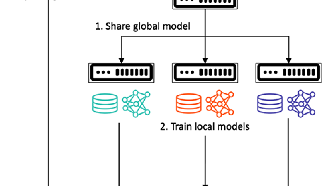
To mitigate these challenges, we propose a federated learning (FL) framework, based on open-source FedML on AWS, which enables analyzing sensitive HCLS data. It involves training a global machine learning (ML) model from distributed health data held locally at different sites. It doesn’t require moving or sharing data across sites or with a centralized server during the model training process.

Deploying an FL framework on the cloud has several challenges. Automating the client-server infrastructure to support multiple accounts or virtual private clouds (VPCs) requires VPC peering and efficient communication across VPCs and instances. In a production workload, a stable deployment pipeline is needed to seamlessly add and remove clients and update their configurations without much overhead. Furthermore, in a heterogenous setup, clients may have varying requirements for compute, network, and storage. In this decentralized architecture, logging and debugging errors across clients can be difficult. Finally, determining the optimal approach to aggregate model parameters, maintain model performance, ensure data privacy, and improve communication efficiency is an arduous task. In this post, we address these challenges by providing a federated learning operations (FLOps) template that hosts a HCLS solution. The solution is agnostic to use cases, which means you can adapt it for your use cases by changing the model and data.

In this two-part series, we demonstrate how you can deploy a cloud-based FL framework on AWS. In the first post, we described FL concepts and the FedML framework. In this second part, we present a proof-of-concept healthcare and life sciences use case from a real-world dataset eICU. This dataset comprises a multi-center critical care database collected from over 200 hospitals, which makes it ideal to test our FL experiments.

HCLS use case

For the purpose of demonstration, we built an FL model on a publicly available dataset to manage critically ill patients. We used the eICU Collaborative Research Database, a multi-center intensive care unit (ICU) database, comprising 200,859 patient unit encounters for 139,367 unique patients. They were admitted to one of 335 units at 208 hospitals located throughout the US between 2014–2015. Due to the underlying heterogeneity and distributed nature of the data, it provides an ideal real-world example to test this FL framework. The dataset includes laboratory measurements, vital signs, care plan information, medications, patient history, admission diagnosis, time-stamped diagnoses from a structured problem list, and similarly chosen treatments. It is available as a set of CSV files, which can be loaded into any relational database system. The tables are de-identified to meet the regulatory requirements US Health Insurance Portability and Accountability Act (HIPAA). The data can be accessed via a PhysioNet repository, and details of the data access process can be found here [1].

The eICU data is ideal for developing ML algorithms, decision support tools, and advancing clinical research. For benchmark analysis, we considered the task of predicting the in-hospital mortality of patients [2]. We defined it as a binary classification task, where each data sample spans a 1-hour window. To create a cohort for this task, we selected patients with a hospital discharge status in the patient’s record and a length of stay of at least 48 hours, because we focus on prediction mortality during the first 24 and 48 hours. This created a cohort of 30,680 patients containing 1,164,966 records. We adopted domain-specific data preprocessing and methods described in [3] for mortality prediction. This resulted in an aggregated dataset comprising several columns per patient per record, as shown in the following figure. The following table provides a patient record in a tabular style interface with time in columns (5 intervals over 48 hours) and vital sign observations in rows. Each row represents a physiological variable, and each column represents its value recorded over a time window of 48 hours for a patient.

We used both numerical and categorical features and grouped all records of each patient to flatten them into a single-record time series. The seven categorical features (Admission diagnosis, Ethnicity, Gender, Glasgow Coma Score Total, Glasgow Coma Score Eyes, Glasgow Coma Score Motor, and Glasgow Coma Score Verbal were converted to one-hot encoding vectors) contained 429 unique values and were converted into one-hot embeddings. To prevent data leakage across training node servers, we split the data by hospital IDs and kept all records of a hospital on a single node.

Solution overview

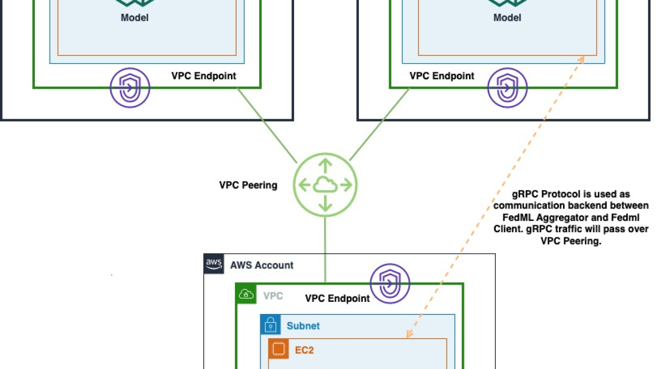
The following diagram shows the architecture of multi-account deployment of FedML on AWS. This includes two clients (Participant A and Participant B) and a model aggregator.

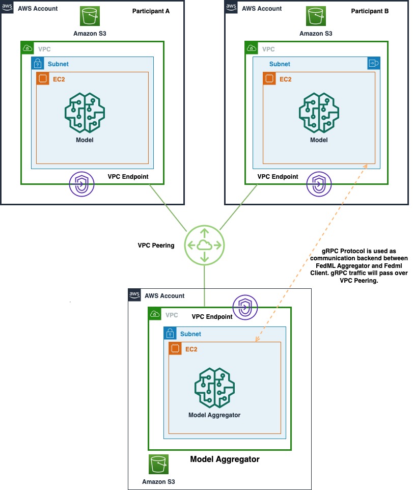
The architecture consists of three separate Amazon Elastic Compute Cloud (Amazon EC2) instances running in its own AWS account. Each of the first two instances is owned by a client, and the third instance is owned by the model aggregator. The accounts are connected via VPC peering to allow ML models and weights to be exchanged between the clients and aggregator. gRPC is used as communication backend for communication between model aggregator and clients. We tested a single account-based distributed computing setup with one server and two client nodes. Each of these instances were created using a custom Amazon EC2 AMI with FedML dependencies installed as per the FedML.ai installation guide.

Set up VPC peering

After you launch the three instances in their respective AWS accounts, you establish VPC peering between the accounts via Amazon Virtual Private Cloud (Amazon VPC). To set up a VPC peering connection, first create a request to peer with another VPC. You can request a VPC peering connection with another VPC in your account, or with a VPC in a different AWS account. To activate the request, the owner of the VPC must accept the request. For the purpose of this demonstration, we set up the peering connection between VPCs in different accounts but the same Region. For other configurations of VPC peering, refer to Create a VPC peering connection.

Before you begin, make sure that you have the AWS account number and VPC ID of the VPC to peer with.

Request a VPC peering connection

To create the VPC peering connection, complete the following steps:

1. On the Amazon VPC console, in the navigation pane, choose Peering connections.
2. Choose Create peering connection.
3. For Peering connection name tag, you can optionally name your VPC peering connection.Doing so creates a tag with a key of the name and a value that you specify. This tag is only visible to you; the owner of the peer VPC can create their own tags for the VPC peering connection.
4. For VPC (Requester), choose the VPC in your account to create the peering connection.
5. For Account, choose Another account.
6. For Account ID, enter the AWS account ID of the owner of the accepter VPC.
7. For VPC (Accepter), enter the VPC ID with which to create the VPC peering connection.
8. In the confirmation dialog box, choose OK.
9. Choose Create peering connection.

Accept a VPC peering connection

As mentioned earlier, the VPC peering connection needs to be accepted by the owner of the VPC the connection request has been sent to. Complete the following steps to accept the peering connection request:

1. On the Amazon VPC console, use the Region selector to choose the Region of the accepter VPC.
2. In the navigation pane, choose Peering connections.
3. Select the pending VPC peering connection (the status is pending-acceptance), and on the Actions menu, choose Accept Request.
4. In the confirmation dialog box, choose Yes, Accept.
5. In the second confirmation dialog, choose Modify my route tables now to go directly to the route tables page, or choose Close to do this later.

Update route tables

To enable private IPv4 traffic between instances in peered VPCs, add a route to the route tables associated with the subnets for both instances. The route destination is the CIDR block (or portion of the CIDR block) of the peer VPC, and the target is the ID of the VPC peering connection. For more information, see Configure route tables.

Update your security groups to reference peer VPC groups

Update the inbound or outbound rules for your VPC security groups to reference security groups in the peered VPC. This allows traffic to flow across instances that are associated with the referenced security group in the peered VPC. For more details about setting up security groups, refer to Update your security groups to reference peer security groups.

Configure FedML

After you have the three EC2 instances running, connect to each of them and perform the following steps:

1. Clone the FedML repository.
2. Provide topology data about your network in the config file grpc_ipconfig.csv.

This file can be found at FedML/fedml_experiments/distributed/fedavg in the FedML repository. The file includes data about the server and clients and their designated node mapping, such as FL Server – Node 0, FL Client 1 – Node 1, and FL Client 2 – Node2.

3. Define the GPU mapping config file.

This file can be found at FedML/fedml_experiments/distributed/fedavg in the FedML repository. The file gpu_mapping.yaml consists of configuration data for client server mapping to the corresponding GPU, as shown in the following snippet.

After you define these configurations, you’re ready to run the clients. Note that the clients must be run before kicking off the server. Before doing that, let’s set up the data loaders for the experiments.

Customize FedML for eICU

To customize the FedML repository for eICU dataset, make the following changes to the data and data loader.

Data

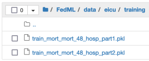
Add data to the pre-assigned data folder, as shown in the following screenshot. You can place the data in any folder of your choice, as long as the path is consistently referenced in the training script and has access enabled. To follow a real-world HCLS scenario, where local data isn’t shared across sites, split and sample the data so there’s no overlap of hospital IDs across the two clients. This ensures the data of a hospital is hosted on its own server. We also enforced the same constraint to split the data into train/test sets within each client. Each of the train/test sets across the clients had a 1:10 ratio of positive to negative labels, with roughly 27,000 samples in training and 3,000 samples in test. We handle the data imbalance in model training with a weighted loss function.

Data loader

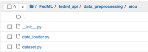
Each of the FedML clients loads the data and converts it into PyTorch tensors for efficient training on GPU. Extend the existing FedML nomenclature to add a folder for eICU data in the data_processing folder.

The following code snippet loads the data from the data source. It preprocesses the data and returns one item at a time through the __getitem__ function.

import logging
import pickle
import random
import numpy as np
import torch.utils.data as data


class eicu_truncated(data.Dataset):

    def __init__(self, file_path, dataidxs=None, transform=None, target_transform=None, 
                 task='mort', ohe=True, cat=True, num=True, n_cat_class=429):
        <code to initialize class variables>

    def _load_data(self, file_path):
        <code to load data files for each client>


    def __getitem__(self, index):
	<code to process data and return input and labels>
        return x.astype(np.float32), y

    def __len__(self):
        return len(self.data)

Training ML models with a single data point at a time is tedious and time-consuming. Model training is typically done on a batch of data points at each client. To implement this, the data loader in the data_loader.py script converts NumPy arrays into Torch tensors, as shown in the following code snippet. Note that FedML provides dataset.py and data_loader.py scripts for both structured and unstructured data that you can use for data-specific alterations, as in any PyTorch project.

import logging
import numpy as np
import torch
import torch.utils.data as data
import torchvision.transforms as transforms
from .dataset import eicu_truncated #load the dataset.py file mentioned above
.
.
.
.
# Use standard FedML functions for data distribution and split here
.
.
.
.
# Invoke load_partition_data function for model training. Adapt this function for your dataset
def load_partition_data_eicu(dataset, train_file, test_file, partition_method, partition_alpha, client_number, batch_size):
	<code to partition eicu data and its aggregated statistics>
    return train_data_num, test_data_num, train_data_global, test_data_global, 
           data_local_num_dict, train_data_local_dict, test_data_local_dict, class_num, net_dataidx_map

Import the data loader into the training script

After you create the data loader, import it into the FedML code for ML model training. Like any other dataset (for example, CIFAR-10 and CIFAR-100), load the eICU data to the main_fedavg.py script in the path FedML/fedml_experiments/distributed/fedavg/. Here, we used the federated averaging (fedavg) aggregation function. You can follow a similar method to set up the main file for any other aggregation function.

from fedml_api.data_preprocessing.cifar100.data_loader import load_partition_data_cifar100
from fedml_api.data_preprocessing.cinic10.data_loader import load_partition_data_cinic10

# For eicu
from fedml_api.data_preprocessing.eicu.data_loader import load_partition_data_eicu

We call the data loader function for eICU data with the following code:

    elif dataset_name == "eicu":
        logging.info("load_data. dataset_name = %s" % dataset_name)
        args.client_num_in_total = 2
        train_data_num, test_data_num, train_data_global, test_data_global, 
        train_data_local_num_dict, train_data_local_dict, test_data_local_dict, 
        class_num, net_dataidx_map = load_partition_data_eicu(dataset=dataset_name, train_file=args.train_file,
                                                  test_file=args.test_file, partition_method=args.partition_method, partition_alpha=args.partition_alpha,
                                                  client_number=args.client_num_in_total, batch_size=args.batch_size)

Define the model

FedML supports several out-of-the-box deep learning algorithms for various data types, such as tabular, text, image, graphs, and Internet of Things (IoT) data. Load the model specific for eICU with input and output dimensions defined based on the dataset. For this proof of concept development, we used a logistic regression model to train and predict the mortality rate of patients with default configurations. The following code snippet shows the updates we made to the main_fedavg.py script. Note that you can also use custom PyTorch models with FedML and import it into the main_fedavg.py script.

if model_name == "lr" and args.dataset == "mnist":
        logging.info("LogisticRegression + MNIST")
        model = LogisticRegression(28 * 28, output_dim)
elif model_name == "lr" and args.dataset == "eicu":
        logging.info("LogisticRegression + eicu")
        model = LogisticRegression(22100, output_dim)
elif model_name == "rnn" and args.dataset == "shakespeare":
        logging.info("RNN + shakespeare")
        model = RNN_OriginalFedAvg()

Run and monitor FedML training on AWS

The following video shows the training process being initialized in each of the clients. After both the clients are listed for the server, create the server training process that performs federated aggregation of models.

To configure the FL server and clients, complete the following steps:

1. Run Client 1 and Client 2.

To run a client, enter the following command with its corresponding node ID. For instance, to run Client 1 with node ID 1, run from the command line:

> sh run_fedavg_cross_zone_eICU.sh 1

2. After both the client instances are started, start the server instance using the same command and the appropriate node ID per your configuration in the grpc_ipconfig.csv file. You can see the model weights being passed to the server from the client instances.

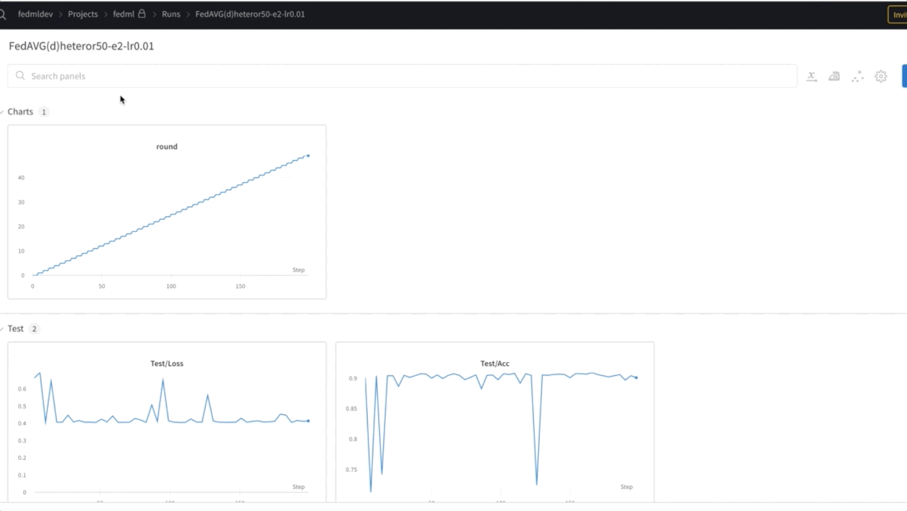
3. We train FL model for 50 epochs. As you can see in the below video, the weights are transferred between nodes 0, 1, and 2, indicating the training is progressing as expected in a federated manner.

4. Finally, monitor and track the FL model training progression across different nodes in the cluster using the weights and biases (wandb) tool, as shown in the following screenshot. Please follow the steps listed here to install wandb and setup monitoring for this solution.
   

The following video captures all these steps to provide an end-to-end demonstration of FL on AWS using FedML:

Conclusion

In this post, we showed how you can deploy an FL framework, based on open-source FedML, on AWS. It allows you to train an ML model on distributed data, without the need to share or move it. We set up a multi-account architecture, where in a real-world scenario, hospitals or healthcare organizations can join the ecosystem to benefit from collaborative learning while maintaining data governance. We used the multi-hospital eICU dataset to test this deployment. This framework can also be applied to other use cases and domains. We will continue to extend this work by automating deployment through infrastructure as code (using AWS CloudFormation), further incorporating privacy-preserving mechanisms, and improving interpretability and fairness of the FL models.

Please review the presentation at re:MARS 2022 focused on “Managed Federated Learning on AWS: A case study for healthcare” for a detailed walkthrough of this solution.

Reference

About the Authors

Vidya Sagar Ravipati is a Manager at the Amazon ML Solutions Lab, where he leverages his vast experience in large-scale distributed systems and his passion for machine learning to help AWS customers across different industry verticals accelerate their AI and cloud adoption. Previously, he was a Machine Learning Engineer in Connectivity Services at Amazon who helped to build personalization and predictive maintenance platforms.

Olivia Choudhury, PhD, is a Senior Partner Solutions Architect at AWS. She helps partners, in the Healthcare and Life Sciences domain, design, develop, and scale state-of-the-art solutions leveraging AWS. She has a background in genomics, healthcare analytics, federated learning, and privacy-preserving machine learning. Outside of work, she plays board games, paints landscapes, and collects manga.

Wajahat Aziz is a Principal Machine Learning and HPC Solutions Architect at AWS, where he focuses on helping healthcare and life sciences customers leverage AWS technologies for developing state-of-the-art ML and HPC solutions for a wide variety of use cases such as Drug Development, Clinical Trials, and Privacy Preserving Machine Learning. Outside of work, Wajahat likes to explore nature, hiking, and reading.

Divya Bhargavi is a Data Scientist and Media and Entertainment Vertical Lead at the Amazon ML Solutions Lab, where she solves high-value business problems for AWS customers using Machine Learning. She works on image/video understanding, knowledge graph recommendation systems, predictive advertising use cases.

Ujjwal Ratan is the leader for AI/ML and Data Science in the AWS Healthcare and Life Science Business Unit and is also a Principal AI/ML Solutions Architect. Over the years, Ujjwal has been a thought leader in the healthcare and life sciences industry, helping multiple Global Fortune 500 organizations achieve their innovation goals by adopting machine learning. His work involving the analysis of medical imaging, unstructured clinical text and genomics has helped AWS build products and services that provide highly personalized and precisely targeted diagnostics and therapeutics. In his free time, he enjoys listening to (and playing) music and taking unplanned road trips with his family.

Chaoyang He is Co-founder and CTO of FedML, Inc., a startup running for a community building open and collaborative AI from anywhere at any scale. His research focuses on distributed/federated machine learning algorithms, systems, and applications. He received his Ph.D. in Computer Science from the University of Southern California, Los Angeles, USA.

Salman Avestimehr is Co-founder and CEO of FedML, Inc., a startup running for a community building open and collaborative AI from anywhere at any scale. Salman Avestimehr is a world-renowned expert in federated learning with over 20 years of R&D leadership in both academia and industry. He is a Dean’s Professor and the inaugural director of the USC-Amazon Center on Trustworthy Machine Learning at the University of Southern California. He has also been an Amazon Scholar in Amazon. He is a United States Presidential award winner for his profound contributions in information                                                  technology, and a Fellow of IEEE.

Read More

Analyzing real-world healthcare and life sciences (HCLS) data poses several practical challenges, such as distributed data silos, lack of sufficient data at any single site for rare events, regulatory guidelines that prohibit data sharing, infrastructure requirement, and cost incurred in creating a centralized data repository. Because they are in a highly regulated domain, HCLS partners and customers seek privacy-preserving mechanisms to manage and analyze large-scale, distributed, and sensitive data.

To mitigate these challenges, we propose using an open-source federated learning (FL) framework called FedML, which enables you to analyze sensitive HCLS data by training a global machine learning model from distributed data held locally at different sites. FL doesn’t require moving or sharing data across sites or with a centralized server during the model training process.

In this two-part series, we demonstrate how you can deploy a cloud-based FL framework on AWS. In the first post, we described FL concepts and the FedML framework. In the second post, we present the use cases and dataset to show its effectiveness in analyzing real-world healthcare datasets, such as the eICU data, which comprises a multi-center critical care database collected from over 200 hospitals.

Background

Although the volume of HCLS-generated data has never been greater, the challenges and constraints associated with accessing such data limits its utility for future research. Machine learning (ML) presents an opportunity to address some of these concerns and is being adopted to advance data analytics and derive meaningful insights from diverse HCLS data for use cases like care delivery, clinical decision support, precision medicine, triage and diagnosis, and chronic care management. Because ML algorithms are often not adequate in protecting the privacy of patient-level data, there is a growing interest among HCLS partners and customers to use privacy-preserving mechanisms and infrastructure for managing and analyzing large-scale, distributed, and sensitive data. [1]

We have developed an FL framework on AWS that enables analyzing distributed and sensitive health data in a privacy-preserving manner. It involves training a shared ML model without moving or sharing data across sites or with a centralized server during the model training process, and can be implemented across multiple AWS accounts. Participants can either choose to maintain their data in their on-premises systems or in an AWS account that they control. Therefore, it brings analytics to data, rather than moving data to analytics.

In this post, we showed how you can deploy the open-source FedML framework on AWS. We test the framework on eICU data, a multi-center critical care database collected from over 200 hospitals, to predict in-hospital patient mortality. We can use this FL framework to analyze other datasets, including genomic and life sciences data. It can also be adopted by other domains that are rife with distributed and sensitive data, including finance and education sectors.

Federated learning

Advancements in technology have led to an explosive growth of data across industries, including HCLS. HCLS organizations often store data in siloes. This poses a major challenge in data-driven learning, which requires large datasets to generalize well and achieve the desired level of performance. Moreover, gathering, curating, and maintaining high-quality datasets incur significant time and cost.

Federated learning mitigates these challenges by collaboratively training ML models that use distributed data, without the need to share or centralize them. It allows diverse sites to be represented within the final model, reducing the potential risk for site-based bias. The framework follows a client-server architecture, where the server shares a global model with the clients. The clients train the model based on local data and share parameters (such as gradients or model weights) with the server. The server aggregates these parameters to update the global model, which is then shared with the clients for next round of training, as shown in the following figure. This iterative process of model training continues until the global model converges.

Iterative process of model training

In recent years, this new learning paradigm has been successfully adopted to address the concern of data governance in training ML models. One such effort is MELLODDY, an Innovative Medicines Initiative (IMI)-led consortium, powered by AWS. It’s a 3-year program involving 10 pharmaceutical companies, 2 academic institutions, and 3 technology partners. Its primary goal is to develop a multi-task FL framework to improve the predictive performance and chemical applicability of drug discovery-based models. The platform comprises multiple AWS accounts, with each pharma partner retaining full control of their respective accounts to maintain their private datasets, and a central ML account coordinating the model training tasks.

The consortium trained models on billions of data points, consisting of over 20 million small molecules in over 40,000 biological assays. Based on experimental results, the collaborative models demonstrated a 4% improvement in categorizing molecules as either pharmacologically or toxicologically active or inactive. It also led to a 10% increase in its ability to yield confident predictions when applied to new types of molecules. Finally, the collaborative models were typically 2% better at estimating values of toxicological and pharmacological activities.

FedML

FedML is an open-source library to facilitate FL algorithm development. It supports three computing paradigms: on-device training for edge devices, distributed computing, and single-machine simulation. It also offers diverse algorithmic research with flexible and generic API design and comprehensive reference baseline implementations (optimizer, models, and datasets). For a detailed description of the FedML library, refer to FedML.

The following figure presents the open-source library architecture of FedML.

Open-source library architecture of FedML

As seen in the preceding figure, from the application point of view, FedML shields details of the underlying code and complex configurations of distributed training. At the application level, such as computer vision, natural language processing, and data mining, data scientists and engineers only need to write the model, data, and trainer in the same way as a standalone program and then pass it to the FedMLRunner object to complete all the processes, as shown in the following code. This greatly reduces the overhead for application developers to perform FL.

import fedml
from my_model_trainer import MyModelTrainer
from my_server_aggregator import MyServerAggregator
from fedml import FedMLRunner

if __name__ == "__main__":
# init FedML framework
args = fedml.init()

# init device
device = fedml.device.get_device(args)

# load data
dataset, output_dim = fedml.data.load(args)

# load model
model = fedml.model.create(args, output_dim)

# my customized trainer and aggregator
trainer = MyModelTrainer(model, args)
aggregator = MyServerAggregator(model, args)

# start training
fedml_runner = FedMLRunner(args, device, dataset, model, trainer, aggregator)
fedml_runner.run()

The FedML algorithm is still a work in progress and constantly being improved. To this end, FedML abstracts the core trainer and aggregator and provides users with two abstract objects, FedML.core.ClientTrainer and FedML.core.ServerAggregator, which only need to inherit the interfaces of these two abstract objects and pass them to FedMLRunner. Such customization provides ML developers with maximum flexibility. You can define arbitrary model structures, optimizers, loss functions, and more. These customizations can also be seamlessly connected with the open-source community, open platform, and application ecology mentioned earlier with the help of FedMLRunner, which completely solves the long lag problem from innovative algorithms to commercialization.

Finally, as shown in the preceding figure, FedML supports distributed computing processes, such as complex security protocols and distributed training as a Directed Acyclic Graph (DAG) flow computing process, making the writing of complex protocols similar to standalone programs. Based on this idea, the security protocol Flow Layer 1 and the ML algorithm process Flow Layer 2 can be easily separated so that security engineers and ML engineers can operate while maintaining a modular architecture.

The FedML open-source library supports federated ML use cases for edge as well as cloud. On the edge, the framework facilitates training and deployment of edge models to mobile phones and internet of things (IoT) devices. In the cloud, it enables global collaborative ML, including multi-Region, and multi-tenant public cloud aggregation servers, as well as private cloud deployment in Docker mode. The framework addresses key concerns with regards to privacy-preserving FL such as security, privacy, efficiency, weak supervision, and fairness.

Conclusion

In this post, we showed how you can deploy the open-source FedML framework on AWS. This allows you to train an ML model on distributed data, without the need to share or move it. We set up a multi-account architecture, where in a real-world scenario, organizations can join the ecosystem to benefit from collaborative learning while maintaining data governance. In the next post, we use the multi-hospital eICU dataset to demonstrate its effectiveness in a real-world scenario.

Please review the presentation at re:MARS 2022 focused on “Managed Federated Learning on AWS: A case study for healthcare” for a detailed walkthrough of this solution.

Reference

About the Authors

Olivia Choudhury, PhD, is a Senior Partner Solutions Architect at AWS. She helps partners, in the Healthcare and Life Sciences domain, design, develop, and scale state-of-the-art solutions leveraging AWS. She has a background in genomics, healthcare analytics, federated learning, and privacy-preserving machine learning. Outside of work, she plays board games, paints landscapes, and collects manga.

Vidya Sagar Ravipati is a Manager at the Amazon ML Solutions Lab, where he leverages his vast experience in large-scale distributed systems and his passion for machine learning to help AWS customers across different industry verticals accelerate their AI and cloud adoption. Previously, he was a Machine Learning Engineer in Connectivity Services at Amazon who helped to build personalization and predictive maintenance platforms.

Wajahat Aziz is a Principal Machine Learning and HPC Solutions Architect at AWS, where he focuses on helping healthcare and life sciences customers leverage AWS technologies for developing state-of-the-art ML and HPC solutions for a wide variety of use cases such as Drug Development, Clinical Trials, and Privacy Preserving Machine Learning. Outside of work, Wajahat likes to explore nature, hiking, and reading.

Divya Bhargavi is a Data Scientist and Media and Entertainment Vertical Lead at the Amazon ML Solutions Lab, where she solves high-value business problems for AWS customers using Machine Learning. She works on image/video understanding, knowledge graph recommendation systems, predictive advertising use cases.

Ujjwal Ratan is the leader for AI/ML and Data Science in the AWS Healthcare and Life Science Business Unit and is also a Principal AI/ML Solutions Architect. Over the years, Ujjwal has been a thought leader in the healthcare and life sciences industry, helping multiple Global Fortune 500 organizations achieve their innovation goals by adopting machine learning. His work involving the analysis of medical imaging, unstructured clinical text and genomics has helped AWS build products and services that provide highly personalized and precisely targeted diagnostics and therapeutics. In his free time, he enjoys listening to (and playing) music and taking unplanned road trips with his family.

Chaoyang He is Co-founder and CTO of FedML, Inc., a startup running for a community building open and collaborative AI from anywhere at any scale. His research focuses on distributed/federated machine learning algorithms, systems, and applications. He received his Ph.D. in Computer Science from the University of Southern California, Los Angeles, USA.

Salman Avestimehr is Professor, the inaugural director of the USC-Amazon Center for Secure and Trusted Machine Learning (Trusted AI), and the director of the Information Theory and Machine Learning (vITAL) research lab at the Electrical and Computer Engineering Department and Computer Science Department of University of Southern California. He is also the co-founder and CEO of FedML. He received my Ph.D. in Electrical Engineering and Computer Sciences from UC Berkeley in 2008. His research focuses on the areas of information theory, decentralized and federated machine learning, secure and privacy-preserving learning and computing.

Read More

This post was co-authored with Mark Lott, Distinguished Technical Architect, Salesforce, Inc.

Enterprises that operate globally are experiencing challenges sourcing customer support professionals with multi-lingual experience. This process can be cost-prohibitive and difficult to scale, leading many enterprises to only support English for chats. Using human interpreters for translation support is expensive, and infeasible since chats need real-time translation. Adding multi-lingual machine translation to these customer support chat workflows provides cost-effective, scalable options that improve the customer experience by providing automated translations for users and agents, create an inclusive customer experience, and improve brand loyalty.

Amazon Translate is a neural machine translation service that delivers fast, high-quality, affordable, and customizable language translation. Service Cloud by Salesforce is one of the world’s most popular and highly rated customer service software solutions. Whether by phone, web, chat, or email, this customer support software enables agents and customers to quickly connect and solve customer problems. AWS and Salesforce have been in a strategic partnership since 2016, and are working together to innovate on behalf of customers.

In this post, we demonstrate how to link Salesforce and AWS in real time and use Amazon Translate from within Service Cloud.

Solution overview

The following diagram shows the solution architecture.

There are two personas. The contact center agent persona uses the Service Cloud console, and the customer persona initiates the chat session via a customer support portal enabled by Salesforce Experience Cloud.

The solution is composed of the following components:

1. A Lightning Web Component that implements a custom header for the customer chat. This component lets the customer toggle between languages.
2. A Lightning Web Component that overrides the chat for the customer and invokes Amazon Translate to translate the text in real time. This is also referred to as a snap-in.
3. An Aura-based web component that provides real-time chat translation services to the call center agent.
4. A Salesforce Apex Callout class, which makes real-time calls to AWS to translate chat messages for the agent and the customer.
5. Amazon API Gateway with AWS Lambda integration that converts the input text to the target language using the Amazon Translate SDK.

Prerequisites

This solution has the following prerequisites:

• An AWS account. If you don’t have one, sign up at https://aws.amazon.com.
• The AWS Cloud Development Kit (AWS CDK) installed and the AWS Command Line Interface (AWS CLI) version 2 installed.
• A Salesforce Trailhead account associated with your Salesforce Developer Edition org.
• Salesforce Code Builder. For installation instructions, refer to Set Up Code Builder.
• Node.js and the npm command line interface.
• Docker.

Deploy resources using the AWS CDK

You can deploy the resources using the AWS CDK, an open-source development framework that lets developers define cloud resources using familiar programming languages. The following steps set up API Gateway, Lambda, and Amazon Translate resources using the AWS CDK. It may take up to 15 minutes to complete the deployment.

1. From a command prompt, run the following commands:

git clone https://github.com/aws-samples/amazon-translate-service-cloud-chat.git
cd amazon-translate-service-cloud-chat/aws
npm i -g aws-cdk
npm i
cdk deploy

2. Take note of the API key and the API endpoint created during the deployment. You need those values later when configuring Salesforce to communicate with API Gateway.

Configure Salesforce Service Cloud

In this section, you use the Service Setup Assistant to enable an out-of-the-box Service Cloud app with optimal settings and layouts. To configure Service Cloud, complete the following steps:

1. Log in to your Salesforce org, choose the gear icon, and choose Service Setup (the purple gear icon).
2. Under Open the Service Setup Assistant, choose Go to Assistant.
3. On the Service Setup Assistant page, in the Turn on your Service app section, toggle Service Setup Assistant to On.

This process may take a couple of minutes to complete. You can choose Check Status to see if the job is finished.

4. When the status shows Ready, choose Get Started.
5. Choose Yes, Let’s Do It.
6. Ignore the Personalize Service section.

At this point, we have enabled Service Cloud.

Enable Salesforce Sites

Salesforce Sites lets you create public websites that are integrated with your Salesforce org. In this step, you register a Salesforce Sites domain, which you customize to embed a chat component that allows the customer persona to engage with the agent. To enable Salesforce Sites, complete the following steps:

1. Log in to your Salesforce org.
2. Choose the gear icon and choose Setup.
3. Under User Interface, choose Sites and Domains, then choose Sites.
4. Select the check box accepting the Sites terms of service and choose Register My Salesforce Site Domain.
5. If a pop-up window appears, choose OK.
6. Make a note of the URL under Sample Domain Name. You need this information in the next step.

Configure Salesforce Chat

In this step, you use Service Setup to configure Salesforce Chat. This walks you through a setup wizard to create chat queues, a team that the agent belongs to, and prioritization. To configure Salesforce Chat, complete the following steps:

1. Choose the gear icon and choose Service Setup.
2. Within the Service Setup home page, choose View All under Recommended Setup.

A dialog box opens with a list of configuration wizards.

3. Choose the Chat with Customers configuration wizard, either by scrolling down or entering chat in the search box, then choose Start.
4. In the Create a chat queue section, enter ChatQueue for Queue Name, and Chat Team for Name This Group.
5. Select yourself as a member of the chat team and choose Next.

This allows your developer edition user account to be an agent within the Service Console.

6. In the Prioritize chats with your other work section, set the ChatQueue priority to 1 and choose Next.
7. In the Adjust your agents’ chat workload section, accept the defaults and choose Next.
8. In the Let’s make chat work on your website section, enter the URL you saved (add https://) and choose Next.
9. In the What’s your type? section, choose Just Contacts, then choose Next.
10. In the In case your team’s busy section, accept the defaults and choose Next.

You don’t need the code snippet because we will drag and drop the predefined chat component in the next section.

11. Choose Next followed by Done.

Configure your customer support digital experience

In this section, you configure the digital experience (the customer persona’s view) to embed a chat widget that the customer will use when they need help. To configure the digital experience, complete the following steps:

1. Choose the gear icon followed by Setup.
2. Under Digital Experiences, choose All Sites.
3. In the Action column under All Sites, choose the Builder link.
4. In the navigation pane, choose Components, and search for chat.
5. Drag Embedded Service Chat to the Content Footer section, which requires you to scroll the window while dragging.
6. You may see a pop-up indicating you cannot access the resources due to a Content Security Policy (CSP) issue. Ignore these errors, and choose OK. We will address these errors in the next step.
   
7. Choose the settings gear in the navigation pane, then choose Security & Privacy.
8. Under Content Security Policy (CSP), change Security Level to Relaxed CSP.
9. Accept any pop-ups asking confirmation and ignore any errors.
10. Under CSP Errors, identify the blocked resources, choose the Allow URL, and choose Allow on any confirmation dialog. This gets rid of the CSP error pop-ups.

11. Close the security setting screen, then choose Publish, then Got it in the resultant dialog.
12. If you continue to get CSP errors, go back to the security settings and manually choose Allow URL for the sites that were blocked under CSP Errors.
13. Choose the Workspaces icon.
14. Choose Administration.
15. Choose Settings, then choose Activate, followed by OK.

Customize Salesforce Chat

You add yourself as a valid user for the CodeBuilder permission set, which lets you create and launch a Salesforce Code Builder project. You then deploy the customizations using the Salesforce CLI. Finally, you (unit) test that the translation is working as intended. To customize chat, complete the following steps:

1. Choose the gear icon and choose Setup.
2. Search for Permission Sets and then choose CodeBuilder on the Permission Sets page.
3. Choose Manage Assignments, followed by Add Assignments.
4. Choose yourself by selecting your name or login.
5. Choose Next, then Assign, then Done.

Your name is now listed under Current Assignments.

6. Under App Launcher, choose Code Builder (Beta).
7. Choose Get Started, followed by New Project.
8. Enter amazon-translate-service for Project Name and Empty for Project Type.
9. Choose Next.
10. Choose Connect a Development Org, then choose Next.
11. If prompted, log in again using the credentials for your development org.
12. Enter amazon-translate-service for Org Alias and choose Create.

It takes a few minutes to create the environment.

13. When the environment is available, choose Launch.
14. On the Terminal tab, enter the following commands:

git init
git remote add origin https://github.com/aws-samples/amazon-translate-service-cloud-chat.git
git fetch origin
git checkout main -f
cd salesforce

15. In the navigation pane, open and edit the file force-app/main/default/externalCredentials/TranslationServiceExtCred.externalCredential-meta.xml.
16. Replace parameterValue of the AuthHeader parameterType to your API key.
17. Save the file.
18. Edit the file force-app/main/default/namedCredentials/ TranslateService.namedCredential-meta.xml.
19. Replace parameterValue of the Url parameterType with your API Gateway URL.
20. Save the file.
21. On the Terminal tab, enter the following commands:

sfdx force:source:deploy --sourcepath ./force-app/main/default
sfdx force:apex:execute -f ./scripts/apex/addUsersToPermSet.apex
sfdx force:apex:execute -f ./scripts/apex/testTranslation.apex

The first command pushes the code and metadata into your Salesforce developer environment:

The second command runs a script that assigns your user to a permission set within your Salesforce developer environment. Each user has to be authorized to use the named credential, which contains the information necessary to connect to AWS.

The last command runs a script that tests the integration between your Salesforce developer environment and the Amazon Translate service. If everything is configured correctly and deployed successfully, you will see that Salesforce can now call Amazon Translate.

Now that we’ve configured, pushed, and tested the project, it’s time to configure the Salesforce user interface to include the translation web components.

22. Choose the gear icon and choose Setup.
23. Under Service, choose Embedded Service, then choose Embedded Service Deployments.
24. For Chat Team, choose View.
25. For Chat Settings¸ choose Edit.
26. Under Customize with Lightning Components, choose Edit.
27. Choose translationHeaderSnapin for Chat Header and translationSnapin for Chat Messages (Text).
28. Choose Save.

Configure the components in the Agent’s desktop interface

You now create a new Lightning app page and add a custom component that displays the translated customer’s messages. To configure agent’s desktop interface, complete the following steps:

1. Choose the gear icon and choose Setup.
2. Choose User Interface, then Lightning App Builder.
3. Choose New in the Lightning Pages section.
4. Choose Record Page, then choose Next.
5. Choose Translation Chat Transcript for Label and Chat Transcript for Object.
6. Choose Next.
7. Choose Header and Two Equal Regions as the page template and choose Finish.
8. Drag the Conversation component into the left-hand view and the TranslationReceiver component into the right-hand view.
9. Choose Save, then choose Activate.
10. Choose Assign as Org Default, then choose Desktop, and Next.
11. Review the assignment and choose Save.
12. Exit from the Lightning App Builder by choosing Save.

Test the translation feature

It’s time to test this feature. It’s easy to test by having two browsers side by side. The first browser is set up as the agent, and the second one as the customer. Make sure you toggle the customer persona’s language as a language other than English, and initiate the chat by choosing Chat with an Expert. Complete the following steps to initiate a conversation:

1. Under App Launcher, choose Service Console.
2. Choose Omni-Channel to open the agent interface.
3. Make yourself available by choosing Available – Chat as your status.
4. Open a separate tab or browser and choose Setup.
5. Choose Digital Experiences, then All Sites.
6. Choose the URL to launch the customer view.
7. Choose Chat with an Expert, and choose the language as es in the drop-down menu at the top of the Chat pane.
8. Provide your name and email.
9. Choose Start Chatting.
10. Go to the agent tab and accept the incoming chat.
11. You can now chat back and forth as a customer speaking Spanish or other supported language and the agent speaking English.

Clean up

To clean up your resources, complete the following steps:

1. Run cdk destroy to delete the provisioned resources.
2. Follow the instructions in Deactivate a Developer Edition Org to deactivate your Salesforce Developer org.

Conclusion

In this post, we demonstrated how you can set up and configure real-time translations powered by Amazon Translate for Salesforce Service Cloud chat conversations. The combination of Salesforce Service Cloud and Amazon Translate enables a scalable, cost-effective solution for your customer support agents to communicate in real time with customers in their preferred languages. Amazon Translate can help you scale this solution to support over 5,550 translation pairs out of the box.

For more details about Amazon Translate, visit Amazon Translate resources to find video resources and blog posts, and also refer to Amazon Translate FAQs. If you’re new to Amazon Translate, try it out using the Free Tier, which offers up to 2 million characters per month for free for the first 12 months, starting from your first translation request.

About the Authors

Mark Lott is a Distinguished Technical Architect at Salesforce. He has over 25 years working in the software industry and works with customers of all sizes to design custom solutions using the Salesforce platform.

Kishore Dhamodaran is a Senior Solutions Architect at AWS. Kishore helps strategic customers with their cloud enterprise strategy and migration journey, leveraging his years of industry and cloud experience.

Tim McLaughlin is a Product Manager at Amazon Web Services in the AWS Language AI Services team. He works closely with customers around the world by supporting their AWS adoption journey with Language AI services.

Jared Wiener is a Solutions Architect at AWS.

Read More

This is guest post by Andy Whittle, Principal Platform Engineer – Application & Reliability Frameworks at The Very Group.

At The Very Group, which operates digital retailer Very, security is a top priority in handling data for millions of customers. Part of how The Very Group secures and tracks business operations is through activity logging between business systems (for example, across the stages of a customer order). It is a critical operating requirement and enables The Very Group to trace incidents and proactively identify problems and trends. However, this can mean processing customer data in the form of personally identifiable information (PII) in relation to activities such as purchases, returns, use of flexible payment options, and account management.

In this post, The Very Group shows how they use Amazon Comprehend to add a further layer of automated defense on top of policies to design threat modelling into all systems, to prevent PII from being sent in log data to Elasticsearch for indexing. Amazon Comprehend is a fully managed and continuously trained natural language processing (NLP) service that can extract insight about the content of a document or text.

Overview of solution

The overriding goal for The Very Group’s engineering team was to prevent any PII data from reaching documents within Elasticsearch. To accomplish this and automate removal of PII from millions of identified records per day, The Very Group’s engineering team created an Application Observability module in Terraform. This module implements an observability solution, including application logs, application performance monitoring (APM), and metrics. Within the module, the team used Amazon Comprehend to highlight PII within log data with the option of removing it before sending to Elasticsearch.

Amazon Comprehend was identified as part of an internal platform engineering initiative to investigate how AWS AI services can be used to improve efficiency and reduce risk in repetitive business activities. The Very Group’s culture to learn and experiment meant Amazon Comprehend was reviewed for applicability using a Java application to learn how it worked with test PII data. The team used code examples in the documentation to accelerate the proof of concept and quickly proved potential within a day.

The engineering team developed a schematic demonstrating how a PII redaction service could integrate with The Very Group’s logging. It involved developing a microservice to call Amazon Comprehend to detect PII data. The solution worked by passing The Very Group’s log data through a Logstash instance running on AWS Fargate, which cleanses the data using another Fargate-hosted pii-logstash-redaction service based on a Spring Boot Java application that makes calls to Amazon Comprehend to remove PII. The following diagram illustrates this architecture.

The Very Group’s solution takes logs from Amazon CloudWatch and Amazon Elastic Container Service (Amazon ECS) and passes cleansed versions to Elasticsearch to be indexed. Amazon Kinesis is used in the solution to capture and store logs for short periods, with Logstash pulling logs down every few seconds.

Logs are sourced across the many business processes, including ordering, returns, and Financial Services. They include logs from over 200 Amazon ECS apps across test and prod environments in Fargate that push logs into Logstash. Another source is AWS Lambda logs that are pulled into Kinesis and then pulled into Logstash. Finally, a separate standalone instance of Filebeat pulls log analysis and that puts them into CloudWatch and then into Logstash. The result is that many sources of logs are pulled or pushed into Logstash and processed by the Application Observability module and Amazon Comprehend before being stored in Elasticsearch.

A separate Terraform module provides all the infrastructure required to stand up a Logstash service capable of exporting logs from CloudWatch log groups into Elasticsearch via an AWS PrivateLink VPC endpoint. The Logstash service can also be integrated with Amazon ECS via a firelens log configuration, with Amazon ECS establishing connectivity over an Amazon Route 53 record. Scalability is built in with Kinesis scaling on demand (although the team started with fixed shards, but are now switching to on-demand usage), and Logstash scales out with additional Amazon Elastic Compute Cloud (Amazon EC2) instances behind an NLB due to protocols used by Filebeat and enables Logstash to more effectively pull logs from Kinesis.

Finally, the Logstash service consists of a task definition containing a Logstash container and PII redaction container, ensuring the removal of PII prior to exporting to Elasticsearch.

Results

The engineering team was able to build and test the solution within a week, without needing to understand machine learning (ML) or the working of AI, using Amazon Comprehend video guidance, API reference documentation, and example code. Having demonstrated business value so quickly, the business product owners have begun to develop new use cases to take advantage of the service. Some decisions had to be made to enable the solution. Although the platform engineering team knew they could redact the data, they wanted to intercept the logs from the current solution (based on a Fluent Bit sidecar to redirect logs to an endpoint). They decided to adopt Logstash to enable interception of log fields through pipelines to integrate with their PII service (comprising the Terraform module and Java service).

The adoption of Logstash was initially done seamlessly. The Very Group engineering squads are now using the service directly through an API endpoint to put logs straight into Elasticsearch. This has allowed them to switch their endpoint from the sidecar to the new endpoint and deploy it through the Terraform module. The only issue the team had was from initial tests that revealed a speed issue when testing with peak trading loads. This was overcome through adjustments to the Java code.

The following code shows how The Very Group use Amazon Comprehend to remove PII from log messages. It detects any PII and creates a list of entity types to record. To accelerate development, the code was taken from the AWS documentation and adapted for use in the Java application service deployed on Fargate.

        
private List<EntityLabel> getEntityLabels(String logData) {
		ContainsPiiEntitiesRequest request = ContainsPiiEntitiesRequest
                .builder()
                .languageCode(LanguageCode.EN)
                .text(logData)
                .build();

        ContainsPiiEntitiesResponse response = comprehendClient.containsPiiEntities(request);

        List<EntityLabel> labels = new ArrayList<>();
        if (response != null && response.hasLabels() && !response.labels().isEmpty()) {
            for (EntityLabel el : response.labels()) {
                if (el.score() > minScore && !redactionConfig.getComprehendExcludedTypes().contains(el.nameAsString())) {
                    labels.add(el);
                }
            }
        }
        return labels;
    }

The following screenshot shows the output sent to Elasticsearch as part of the PII redaction process. The service generates 1 million records per day, generating a record each time a redaction is made.

The log message is redacted, and the field redacted_entities contains a list of the entity types found in the message. In this case, the example found a URL, but it could have identified any type of PII data largely based on the built-in types of PII. An additional bespoke PII type for customer account number was added through Amazon Comprehend, but has not been needed so far. Engineering squad-level overrides are documented in GitHub on how to use them.

Conclusion

This project allowed The Very Group to implement a quick and simple solution to redact sensitive PII in logs. The engineering team added further flexibility allowing overrides for entity types, using Amazon Comprehend to provide the flexibility to redact PII based on the business needs. In the future, the engineering team is looking into training individual Amazon Comprehend entities to redact strings such as our customer IDs.

The result of the solution is that The Very Group has freedom to put logs through without needing to worry. It enforces the policy of not having PII stored in logs, thereby reducing risk and improving compliance. Furthermore, metadata being redacted is being reported back to the business through an Elasticsearch dashboard, enabling alerts and further action.

Make time to assess AWS AI/ML services that your organization hasn’t used yet and foster a culture of experimentation. Starting simple can quickly lead to business benefit, just as The Very Group proved.

About the Author

Andy Whittle is Principal Platform Engineer – Application & Reliability Frameworks at The Very Group, which operates UK-based digital retailer Very. Andy helps deliver performance monitoring across the organization’s tribes, and has a particular interest in application monitoring, observability, and performance. Since joining Very in 1998, Andy has undertaken a wide variety of roles covering content management and catalog production, stock management, production support, DevOps, and Fusion Middleware. For the past 4 years, he has been part of the platform engineering team.

Read More

This post is co-authored by Marios Skevofylakas, Jason Ramchandani and Haykaz Aramyan from Refinitiv, An LSEG Business.

Financial service providers often need to identify relevant news, analyze it, extract insights, and take actions in real time, like trading specific instruments (such as commodities, shares, funds) based on additional information or context of the news item. One such additional piece of information (which we use as an example in this post) is the sentiment of the news.

Refinitiv Data (RD) Libraries provide a comprehensive set of interfaces for uniform access to the Refinitiv Data Catalogue. The library offers multiple layers of abstraction providing different styles and programming techniques suitable for all developers, from low-latency, real-time access to batch ingestions of Refinitiv data.

In this post, we present a prototype AWS architecture that ingests our news feeds using RD Libraries and enhances them with machine learning (ML) model predictions using Amazon SageMaker, a fully managed ML service from AWS.

In an effort to design a modular architecture that could be used in a variety of use cases, like sentiment analysis, named entity recognition, and more, regardless of the ML model used for enhancement, we decided to focus on the real-time space. The reason for this decision is that real-time use cases are generally more complex and that the same architecture can also be used, with minimal adjustments, for batch inference. In our use case, we implement an architecture that ingests our real-time news feed, calculates sentiment on each news headline using ML, and re-serves the AI enhanced feed through a publisher/subscriber architecture.

Moreover, to present a comprehensive and reusable way to productionize ML models by adopting MLOps practices, we introduce the concept of infrastructure as code (IaC) during the entire MLOps lifecycle of the prototype. By using Terraform and a single entry point configurable script, we are able to instantiate the entire infrastructure, in production mode, on AWS in just a few minutes.

In this solution, we don’t address the MLOps aspect of the development, training, and deployment of the individual models. If you’re interested in learning more on this, refer to MLOps foundation roadmap for enterprises with Amazon SageMaker, which explains in detail a framework for model building, training, and deployment following best practices.

Solution overview

In this prototype, we follow a fully automated provisioning methodology in accordance with IaC best practices. IaC is the process of provisioning resources programmatically using automated scripts rather than using interactive configuration tools. Resources can be both hardware and needed software. In our case, we use Terraform to accomplish the implementation of a single configurable entry point that can automatically spin up the entire infrastructure we need, including security and access policies, as well as automated monitoring. With this single entry point that triggers a collection of Terraform scripts, one per service or resource entity, we can fully automate the lifecycle of all or parts of the components of the architecture, allowing us to implement granular control both on the DevOps as well as the MLOps side. After Terraform is correctly installed and integrated with AWS, we can replicate most operations that can be done on the AWS service dashboards.

The following diagram illustrates our solution architecture.

The architecture consists of three stages: ingestion, enrichment, and publishing. During the first stage, the real-time feeds are ingested on an Amazon Elastic Compute Cloud (Amazon EC2) instance that is created through a Refinitiv Data Library-ready AMI. The instance also connects to a data stream via Amazon Kinesis Data Streams, which triggers an AWS Lambda function.

In the second stage, the Lambda function that is triggered from Kinesis Data Streams connects to and sends the news headlines to a SageMaker FinBERT endpoint, which returns the calculated sentiment for the news item. This calculated sentiment is the enrichment in the real-time data that the Lambda function then wraps the news item with and stores in an Amazon DynamoDB table.

In the third stage of the architecture, a DynamoDB stream triggers a Lambda function on new item inserts, which is integrated with an Amazon MQ server running RabbitMQ, which re-serves the AI enhanced stream.

The decision on this three-stage engineering design, rather than the first Lambda layer directly communicating with the Amazon MQ server or implementing more functionality in the EC2 instance, was made to enable exploration of more complex, less coupled AI design architectures in the future.

Building and deploying the prototype

We present this prototype in a series of three detailed blueprints. In each blueprint and for every service used, you will find overviews and relevant information on its technical implementations as well as Terraform scripts that allow you to automatically start, configure, and integrate the service with the rest of the structure. At the end of each blueprint, you will find instructions on how to make sure that everything is working as expected up to each stage. The blueprints are as follows:

• Blueprint I – Real-time news ingestion using Amazon EC2 and Kinesis Data Streams
• Blueprint II – Real-time serverless AI news sentiment analysis using Kinesis Data Streams, Lambda, and SageMaker
• Blueprint III – Real-time streaming using Amazon DynamoDB Streams, Lambda, and Amazon MQ

To start the implementation of this prototype, we suggest creating a new Python environment dedicated to it and installing the necessary packages and tools separately from other environments you may have. To do so, create and activate the new environment in Anaconda using the following commands:

conda create —name rd_news_aws_terraform python=3.7
conda activate rd_news_aws_terraform

We’re now ready to install the AWS Command Line Interface (AWS CLI) toolset that will allow us to build all the necessary programmatic interactions in and between AWS services:

pip install awscli

Now that the AWS CLI is installed, we need to install Terraform. HashiCorp provides Terraform with a binary installer, which you can download and install.

After you have both tools installed, ensure that they properly work using the following commands:

terraform -help
AWS – version

You’re now ready to follow the detailed blueprints on each of the three stages of the implementation.

Blueprint I: Real-time news ingestion using Amazon EC2 and Kinesis Data Streams

This blueprint represents the initial stages of the architecture that allow us to ingest the real-time news feeds. It consists of the following components:

• Amazon EC2 preparing your instance for RD News ingestion – This section sets up an EC2 instance in a way that it enables the connection to the RD Libraries API and the real-time stream. We also show how to save the image of the created instance to ensure its reusability and scalability.
• Real-time news ingestion from Amazon EC2 – A detailed implementation of the configurations needed to enable Amazon EC2 to connect the RD Libraries as well as the scripts to start the ingestion.
• Creating and launching Amazon EC2 from the AMI – Launch a new instance by simultaneously transferring ingestion files to the newly created instance, all automatically using Terraform.
• Creating a Kinesis data stream – This section provides an overview of Kinesis Data Streams and how to set up a stream on AWS.
• Connecting and pushing data to Kinesis – Once the ingestion code is working, we need to connect it and send data to a Kinesis stream.
• Testing the prototype so far – We use Amazon CloudWatch and command line tools to verify that the prototype is working up to this point and that we can continue to the next blueprint. The log of ingested data should look like the following screenshot.

Blueprint II: Real-time serverless AI news sentiment analysis using Kinesis Data Streams, Lambda, and SageMaker

In this second blueprint, we focus on the main part of the architecture: the Lambda function that ingests and analyzes the news item stream, attaches the AI inference to it, and stores it for further use. It includes the following components:

• Lambda – Define a Terraform Lambda configuration allowing it to connect to a SageMaker endpoint.
• Amazon S3 – To implement Lambda, we need to upload the appropriate code to Amazon Simple Storage Service (Amazon S3) and allow the Lambda function to ingest it in its environment. This section describes how we can use Terraform to accomplish that.
• Implementing the Lambda function: Step 1, Handling the Kinesis event – In this section, we start building the Lambda function. Here, we build the Kinesis data stream response handler part only.
• SageMaker – In this prototype, we use a pre-trained Hugging Face model that we store into a SageMaker endpoint. Here, we present how this can be achieved using Terraform scripts and how the appropriate integrations take place to allow SageMaker endpoints and Lambda functions work together.
  • At this point, you can instead use any other model that you have developed and deployed behind a SageMaker endpoint. Such a model could provide a different enhancement to the original news data, based on your needs. Optionally, this can be extrapolated to multiple models for multiple enhancements if such exist. Thanks to the rest of the architecture, any such models will enrich your data sources in real time.
• Building the Lambda function: Step 2, Invoking the SageMaker endpoint – In this section, we build up our original Lambda function by adding the SageMaker block to get a sentiment enhanced news headline by invoking the SageMaker endpoint.
• DynamoDB – Finally, when the AI inference is in the memory of the Lambda function, it re-bundles the item and sends it to a DynamoDB table for storage. Here, we discuss both the appropriate Python code needed to accomplish that, as well as the necessary Terraform scripts that enable these interactions.
• Building the Lambda function: Step 3, Pushing enhanced data to DynamoDB – Here, we continue building up our Lambda function by adding the last part that creates an entry in the Dynamo table.
• Testing the prototype so far – We can navigate to the DynamoDB table on the DynamoDB console to verify that our enhancements are appearing in the table.

Blueprint III: Real-time streaming using DynamoDB Streams, Lambda, and Amazon MQ

This third Blueprint finalizes this prototype. It focuses on redistributing the newly created, AI enhanced data item to a RabbitMQ server in Amazon MQ, allowing consumers to connect and retrieve the enhanced news items in real time. It includes the following components:

• DynamoDB Streams – When the enhanced news item is in DynamoDB, we set up an event getting triggered that can then be captured from the appropriate Lambda function.
• Writing the Lambda producer – This Lambda function captures the event and acts as a producer of the RabbitMQ stream. This new function introduces the concept of Lambda layers as it uses Python libraries to implement the producer functionality.
• Amazon MQ and RabbitMQ consumers – The final step of the prototype is setting up the RabbitMQ service and implementing an example consumer that will connect to the message stream and receive the AI enhanced news items.
• Final test of the prototype – We use an end-to-end process to verify that the prototype is fully working, from ingestion to re-serving and consuming the new AI-enhanced stream.

At this stage, you can validate that everything has been working by navigating to the RabbitMQ dashboard, as shown in the following screenshot.

In the final blueprint, you also find a detailed test vector to make sure that the entire architecture is behaving as planned.

Conclusion

In this post, we shared a solution using ML on the cloud with AWS services like SageMaker (ML), Lambda (serverless), and Kinesis Data Streams (streaming) to enrich streaming news data provided by Refinitiv Data Libraries. The solution adds a sentiment score to news items in real time and scales the infrastructure using code.

The benefit of this modular architecture is that you can reuse it with your own model to perform other types of data augmentation, in a serverless, scalable, and cost-efficient way that can be applied on top of Refinitiv Data Library. This can add value for trading/investment/risk management workflows.

If you have any comments or questions, please leave them in the comments section.

Related Information

• AI Landing page
• Refinitiv Data Library for Python

 About the Authors

Marios Skevofylakas comes from a financial services, investment banking and consulting technology background. He holds an engineering Ph.D. in Artificial Intelligence and an M.Sc. in Machine Vision. Throughout his career, he has participated in numerous multidisciplinary AI and DLT projects. He is currently a Developer Advocate with Refinitiv, an LSEG business, focusing on AI and Quantum applications in financial services.

Jason Ramchandani has worked at Refinitiv, an LSEG Business, for 8 years as Lead Developer Advocate helping to build their Developer Community. Previously he has worked in financial markets for over 15 years with a quant background in the equity/equity-linked space at Okasan Securities, Sakura Finance and Jefferies LLC. His alma mater is UCL.

Haykaz Aramyan comes from a finance and technology background. He holds a Ph.D. in Finance, and an M.Sc. in Finance, Technology and Policy. Through 10 years of professional experience Haykaz worked on several multidisciplinary projects involving pension, VC funds and technology startups. He is currently a Developer Advocate with Refinitiv, An LSEG Business, focusing on AI applications in financial services.

Georgios Schinas is a Senior Specialist Solutions Architect for AI/ML in the EMEA region. He is based in London and works closely with customers in UK and Ireland. Georgios helps customers design and deploy machine learning applications in production on AWS with a particular interest in MLOps practices and enabling customers to perform machine learning at scale. In his spare time, he enjoys traveling, cooking and spending time with friends and family.

Muthuvelan Swaminathan is an Enterprise Solutions Architect based out of New York. He works with enterprise customers providing architectural guidance in building resilient, cost-effective, innovative solutions that address their business needs and help them execute at scale using AWS products and services.

Mayur Udernani leads AWS AI & ML business with commercial enterprises in UK & Ireland. In his role, Mayur spends majority of his time with customers and partners to help create impactful solutions that solve the most pressing needs of a customer or for a wider industry leveraging AWS Cloud, AI & ML services. Mayur lives in the London area. He has an MBA from Indian Institute of Management and Bachelors in Computer Engineering from Mumbai University.

Read More

Amazon SageMaker is a fully managed machine learning (ML) service. With SageMaker, data scientists and developers can quickly and easily build and train ML models, and then directly deploy them into a production-ready hosted environment. It provides an integrated Jupyter authoring notebook instance for easy access to your data sources for exploration and analysis, so you don’t have to manage servers. It also provides common ML algorithms that are optimized to run efficiently against extremely large data in a distributed environment.

SageMaker real-time inference is ideal for workloads that have real-time, interactive, low-latency requirements. With SageMaker real-time inference, you can deploy REST endpoints that are backed by a specific instance type with a certain amount of compute and memory. Deploying a SageMaker real-time endpoint is only the first step in the path to production for many customers. We want to be able to maximize the performance of the endpoint to achieve a target transactions per second (TPS) while adhering to latency requirements. A large part of performance optimization for inference is making sure you select the proper instance type and count to back an endpoint.

This post describes the best practices for load testing a SageMaker endpoint to find the right configuration for the number of instances and size. This can help us understand the minimum provisioned instance requirements to meet our latency and TPS requirements. From there, we dive into how you can track and understand the metrics and performance of the SageMaker endpoint utilizing Amazon CloudWatch metrics.

We first benchmark the performance of our model on a single instance to identify the TPS it can handle per our acceptable latency requirements. Then we extrapolate the findings to decide on the number of instances we need in order to handle our production traffic. Finally, we simulate production-level traffic and set up load tests for a real-time SageMaker endpoint to confirm our endpoint can handle the production-level load. The entire set of code for the example is available in the following GitHub repository.

Overview of solution

For this post, we deploy a pre-trained Hugging Face DistilBERT model from the Hugging Face Hub. This model can perform a number of tasks, but we send a payload specifically for sentiment analysis and text classification. With this sample payload, we strive to achieve 1000 TPS.

Deploy a real-time endpoint

This post assumes you are familiar with how to deploy a model. Refer to Create your endpoint and deploy your model to understand the internals behind hosting an endpoint. For now, we can quickly point to this model in the Hugging Face Hub and deploy a real-time endpoint with the following code snippet:

# Hub Model configuration. https://huggingface.co/models
hub = {
'HF_MODEL_ID':'distilbert-base-uncased',
'HF_TASK':'text-classification'
}

# create Hugging Face Model Class
huggingface_model = HuggingFaceModel(
transformers_version='4.17.0',
pytorch_version='1.10.2',
py_version='py38',
env=hub,
role=role,
)

# deploy model to SageMaker Inference
predictor = huggingface_model.deploy(
initial_instance_count=1, # number of instances
instance_type='ml.m5.12xlarge' # ec2 instance type
)

Let’s test our endpoint quickly with the sample payload that we want to use for load testing:

import boto3
import json
client = boto3.client('sagemaker-runtime')
content_type = "application/json"
request_body = {'inputs': "I am super happy right now."}
data = json.loads(json.dumps(request_body))
payload = json.dumps(data)
response = client.invoke_endpoint(
EndpointName=predictor.endpoint_name,
ContentType=content_type,
Body=payload)
result = response['Body'].read()
result

Note that we’re backing the endpoint using a single Amazon Elastic Compute Cloud (Amazon EC2) instance of type ml.m5.12xlarge, which contains 48 vCPU and 192 GiB of memory. The number of vCPUs is a good indication of the concurrency the instance can handle. In general, it’s recommended to test different instance types to make sure we have an instance that has resources that are properly utilized. To see a full list of SageMaker instances and their corresponding compute power for real-time Inference, refer to Amazon SageMaker Pricing.

Metrics to track

Before we can get into load testing, it’s essential to understand what metrics to track to understand the performance breakdown of your SageMaker endpoint. CloudWatch is the primary logging tool that SageMaker uses to help you understand the different metrics that describe your endpoint’s performance. You can utilize CloudWatch logs to debug your endpoint invocations; all logging and print statements you have in your inference code are captured here. For more information, refer to How Amazon CloudWatch works.

There are two different types of metrics CloudWatch covers for SageMaker: instance-level and invocation metrics.

Instance-level metrics

The first set of parameters to consider is the instance-level metrics: CPUUtilization and MemoryUtilization (for GPU-based instances, GPUUtilization). For CPUUtilization, you may see percentages above 100% at first in CloudWatch. It’s important to realize for CPUUtilization, the sum of all the CPU cores is being displayed. For example, if the instance behind your endpoint contains 4 vCPUs, this means the range of utilization is up to 400%. MemoryUtilization, on the other hand, is in the range of 0–100%.

Specifically, you can use CPUUtilization to get a deeper understanding of if you have sufficient or even an excess amount of hardware. If you have an under-utilized instance (less than 30%), you could potentially scale down your instance type. Conversely, if you are around 80–90% utilization, it would benefit to pick an instance with greater compute/memory. From our tests, we suggest around 60–70% utilization of your hardware.

Invocation metrics

As suggested by the name, invocation metrics is where we can track the end-to-end latency of any invokes to your endpoint. You can utilize the invocation metrics to capture error counts and what type of errors (5xx, 4xx, and so on) that your endpoint may be experiencing. More importantly, you can understand the latency breakdown of your endpoint calls. A lot of this can be captured with ModelLatency and OverheadLatency metrics, as illustrated in the following diagram.

The ModelLatency metric captures the time that inference takes within the model container behind a SageMaker endpoint. Note that the model container also includes any custom inference code or scripts that you have passed for inference. This unit is captured in microseconds as an invocation metric, and generally you can graph a percentile across CloudWatch (p99, p90, and so on) to see if you’re meeting your target latency. Note that several factors can impact model and container latency, such as the following:

• Custom inference script – Whether you have implemented your own container or used a SageMaker-based container with custom inference handlers, it’s best practice to profile your script to catch any operations that are specifically adding a lot of time to your latency.
• Communication protocol – Consider REST vs. gRPC connections to the model server within the model container.
• Model framework optimizations – This is framework specific, for example with TensorFlow, there are a number of environment variables you can tune that are TF Serving specific. Make sure to check what container you’re using and if there are any framework-specific optimizations you can add within the script or as environment variables to inject in the container.

OverheadLatency is measured from the time that SageMaker receives the request until it returns a response to the client, minus the model latency. This part is largely outside of your control and falls under the time taken by SageMaker overheads.

End-to-end latency as a whole depends on a variety of factors and isn’t necessarily the sum of ModelLatency plus OverheadLatency. For example, if you client is making the InvokeEndpoint API call over the internet, from the client’s perspective, the end-to-end latency would be internet + ModelLatency + OverheadLatency. As such, when load testing your endpoint in order to accurately benchmark the endpoint itself, it’s recommended to focus on the endpoint metrics (ModelLatency, OverheadLatency, and InvocationsPerInstance) to accurately benchmark the SageMaker endpoint. Any issues related to end-to-end latency can then be isolated separately.

A few questions to consider for end-to-end latency:

• Where is the client that is invoking your endpoint?
• Are there any intermediary layers between your client and the SageMaker runtime?

Auto scaling

We don’t cover auto scaling in this post specifically, but it’s an important consideration in order to provision the correct number of instances based on the workload. Depending on your traffic patterns, you can attach an auto scaling policy to your SageMaker endpoint. There are different scaling options, such as TargetTrackingScaling, SimpleScaling, and StepScaling. This allows your endpoint to scale in and out automatically based on your traffic pattern.

A common option is target tracking, where you can specify a CloudWatch metric or custom metric that you have defined and scale out based on that. A frequent utilization of auto scaling is tracking the InvocationsPerInstance metric. After you have identified a bottleneck at a certain TPS, you can often use that as a metric to scale out to a greater number of instances to be able to handle peak loads of traffic. To get a deeper breakdown of auto scaling SageMaker endpoints, refer to Configuring autoscaling inference endpoints in Amazon SageMaker.

Load testing

Although we utilize Locust to display how we can load test at scale, if you’re trying to right size the instance behind your endpoint, SageMaker Inference Recommender is a more efficient option. With third-party load testing tools, you have to manually deploy endpoints across different instances. With Inference Recommender, you can simply pass an array of the instance types you want to load test against, and SageMaker will spin up jobs for each of these instances.

Locust

For this example, we use Locust, an open-source load testing tool that you can implement using Python. Locust is similar to many other open-source load testing tools, but has a few specific benefits:

• Easy to set up – As we demonstrate in this post, we’ll pass a simple Python script that can easily be refactored for your specific endpoint and payload.
• Distributed and scalable – Locust is event-based and utilizes gevent under the hood. This is very useful for testing highly concurrent workloads and simulating thousands of concurrent users. You can achieve high TPS with a single process running Locust, but it also has a distributed load generation feature that enables you to scale out to multiple processes and client machines, as we will explore in this post.
• Locust metrics and UI – Locust also captures end-to-end latency as a metric. This can help supplement your CloudWatch metrics to paint a full picture of your tests. This is all captured in the Locust UI, where you can track concurrent users, workers, and more.

To further understand Locust, check out their documentation.

Amazon EC2 setup

You can set up Locust in whatever environment is compatible for you. For this post, we set up an EC2 instance and install Locust there to conduct our tests. We use a c5.18xlarge EC2 instance. The client-side compute power is also something to consider. At times when you run out of compute power on the client side, this is often not captured, and is mistaken as a SageMaker endpoint error. It’s important to place your client in a location of sufficient compute power that can handle the load that you are testing at. For our EC2 instance, we use an Ubuntu Deep Learning AMI, but you can utilize any AMI as long as you can properly set up Locust on the machine. To understand how to launch and connect to your EC2 instance, refer to the tutorial Get started with Amazon EC2 Linux instances.

The Locust UI is accessible via port 8089. We can open this by adjusting our inbound security group rules for the EC2 Instance. We also open up port 22 so we can SSH into the EC2 instance. Consider scoping the source down to the specific IP address you are accessing the EC2 instance from.

After you’re connected to your EC2 instance, we set up a Python virtual environment and install the open-source Locust API via the CLI:

virtualenv venv #venv is the virtual environment name, you can change as you desire
source venv/bin/activate #activate virtual environment
pip install locust

We’re now ready to work with Locust for load testing our endpoint.

Locust testing

All Locust load tests are conducted based off of a Locust file that you provide. This Locust file defines a task for the load test; this is where we define our Boto3 invoke_endpoint API call. See the following code:

config = Config(
retries = {
'max_attempts': 0,
'mode': 'standard'
}
)

self.sagemaker_client = boto3.client('sagemaker-runtime',config=config)
self.endpoint_name = host.split('/')[-1]
self.region = region
self.content_type = content_type
self.payload = payload

In the preceding code, adjust your invoke endpoint call parameters to suit your specific model invocation. We use the InvokeEndpoint API using the following piece of code in the Locust file; this is our load test run point. The Locust file we’re using is locust_script.py.

def send(self):

request_meta = {
"request_type": "InvokeEndpoint",
"name": "SageMaker",
"start_time": time.time(),
"response_length": 0,
"response": None,
"context": {},
"exception": None,
}
start_perf_counter = time.perf_counter()

try:
response = self.sagemaker_client.invoke_endpoint(
EndpointName=self.endpoint_name,
Body=self.payload,
ContentType=self.content_type
)
response_body = response["Body"].read()

Now that we have our Locust script ready, we want to run distributed Locust tests to stress test our single instance to find out how much traffic our instance can handle.

Locust distributed mode is a little more nuanced than a single-process Locust test. In distributed mode, we have one primary and multiple workers. The primary worker instructs the workers on how to spawn and control the concurrent users that are sending a request. In our distributed.sh script, we see by default that 240 users will be distributed across the 60 workers. Note that the --headless flag in the Locust CLI removes the UI feature of Locust.

#replace with your endpoint name in format https://<<endpoint-name>>
export ENDPOINT_NAME=https://$1

export REGION=us-east-1
export CONTENT_TYPE=application/json
export PAYLOAD='{"inputs": "I am super happy right now."}'
export USERS=240
export WORKERS=60
export RUN_TIME=1m
export LOCUST_UI=false # Use Locust UI

.
.
.

locust -f $SCRIPT -H $ENDPOINT_NAME --master --expect-workers $WORKERS -u $USERS -t $RUN_TIME --csv results &
.
.
.

for (( c=1; c<=$WORKERS; c++ ))
do
locust -f $SCRIPT -H $ENDPOINT_NAME --worker --master-host=localhost &
done

./distributed.sh huggingface-pytorch-inference-2022-10-04-02-46-44-677 #to execute Distributed Locust test

We first run the distributed test on a single instance backing the endpoint. The idea here is we want to fully maximize a single instance to understand the instance count we need to achieve our target TPS while staying within our latency requirements. Note that if you want to access the UI, change the Locust_UI environment variable to True and take the public IP of your EC2 instance and map port 8089 to the URL.

The following screenshot shows our CloudWatch metrics.

Eventually, we notice that although we initially achieve a TPS of 200, we start noticing 5xx errors in our EC2 client-side logs, as shown in the following screenshot.

We can also verify this by looking at our instance-level metrics, specifically CPUUtilization.

Here we notice CPUUtilization at nearly 4,800%. Our ml.m5.12x.large instance has 48 vCPUs (48 * 100 = 4800~). This is saturating the entire instance, which also helps explain our 5xx errors. We also see an increase in ModelLatency.

It seems as if our single instance is getting toppled and doesn’t have the compute to sustain a load past the 200 TPS that we are observing. Our target TPS is 1000, so let’s try to increase our instance count to 5. This might have to be even more in a production setting, because we were observing errors at 200 TPS after a certain point.

We see in both the Locust UI and CloudWatch logs that we have a TPS of nearly 1000 with five instances backing the endpoint.

If you start experiencing errors even with this hardware setup, make sure to monitor CPUUtilization to understand the full picture behind your endpoint hosting. It’s crucial to understand your hardware utilization to see if you need to scale up or even down. Sometimes container-level problems lead to 5xx errors, but if CPUUtilization is low, it indicates that it’s not your hardware but something at the container or model level that might be leading to these issues (proper environment variable for number of workers not set, for example). On the other hand, if you notice your instance is getting fully saturated, it’s a sign that you need to either increase the current instance fleet or try out a larger instance with a smaller fleet.

Although we increased the instance count to 5 to handle 100 TPS, we can see that the ModelLatency metric is still high. This is due to the instances being saturated. In general, we suggest aiming to utilize the instance’s resources between 60–70%.

Clean up

After load testing, make sure to clean up any resources you won’t utilize via the SageMaker console or through the delete_endpoint Boto3 API call. In addition, make sure to stop your EC2 instance or whatever client setup you have to not incur any further charges there as well.

Summary

In this post, we described how you can load test your SageMaker real-time endpoint. We also discussed what metrics you should be evaluating when load testing your endpoint to understand your performance breakdown. Make sure to check out SageMaker Inference Recommender to further understand instance right-sizing and more performance optimization techniques.

About the Authors

Marc Karp is a ML Architect with the SageMaker Service team. He focuses on helping customers design, deploy and manage ML workloads at scale. In his spare time, he enjoys traveling and exploring new places.

Ram Vegiraju is a ML Architect with the SageMaker Service team. He focuses on helping customers build and optimize their AI/ML solutions on Amazon SageMaker. In his spare time, he loves traveling and writing.

Read More

If you’ve had the opportunity to build a search application for unstructured data (i.e., wiki, informational web sites, self-service help pages, internal documentation, etc.) using open source or commercial-off-the-shelf search engines, then you’re probably familiar with the inherent accuracy challenges involved in getting relevant search results. The intended meaning of both query and document can be lost because the search is reduced to matching component keywords and terms. Consequently, while you get results that may contain the right words, they aren’t always relevant to the user. You need your search engine to be smarter so it can rank documents based on matching the meaning or semantics of the content to the intention of the user’s query.

Amazon Kendra provides a fully managed intelligent search service that automates document ingestion and provides highly accurate search and FAQ results based on content across many data sources. If you haven’t migrated to Amazon Kendra and would like to improve the quality of search results, you can use Amazon Kendra Intelligent Ranking for self-managed OpenSearch on your existing search solution.

We’re delighted to introduce the new Amazon Kendra Intelligent Ranking for self-managed OpenSearch, and its companion plugin for the OpenSearch search engine! Now you can easily add intelligent ranking to your OpenSearch document queries, with no need to migrate, duplicate your OpenSearch indexes, or rewrite your applications. The difference between Amazon Kendra Intelligent Ranking for self-managed OpenSearch and the fully managed Amazon Kendra service is that while the former provides powerful semantic re-ranking for the search results, the later provides additional search accuracy improvements and functionality such as incremental learning, question answering, FAQ matching, and built-in connectors. For more information about the fully managed service, please visit the Amazon Kendra service page.

With Amazon Kendra Intelligent Ranking for self-managed OpenSearch, previous results like this:

Query: What is the address of the White House?

Hit1 (best): The president delivered an address to the nation from the White House today.

Hit2: The White House is located at: 1600 Pennsylvania Avenue NW, Washington, DC 20500

become like this: 

Query: What is the address of the White House?

Hit1 (best): The White House is located at: 1600 Pennsylvania Avenue NW, Washington, DC 20500

Hit2: The president delivered an address to the nation from the White House today.

In this post, we show you how to get started with Amazon Kendra Intelligent Ranking for self-managed OpenSearch, and we provide a few examples that demonstrate the power and value of this feature.

Components of Amazon Kendra Intelligent Ranking for self-managed OpenSearch

• Amazon Kendra Intelligent Ranking application programming interface (API) – The functions from this API are used to perform tasks related to provisioning execution plans and semantic re-ranking of your search results.
• Amazon Kendra Intelligent Ranking plugin for self-managed OpenSearch – This is installed along with your OpenSearch deployment and uses the Rescore function of the Amazon Kendra Intelligent Ranking API to semantically re-rank the search results.
• OpenSearch Dashboards Compare Search Results Plugin – This lets you compare search results from two queries side by side, for example, where one query is a keyword search, while the other query uses Amazon Kendra Intelligent Ranking for self-managed OpenSearch.

Prerequisites

For this tutorial, you’ll need a bash terminal on Linux, Mac, or Windows Subsystem for Linux, and an AWS account. Hint: consider using an Amazon Cloud9 instance or an Amazon Elastic Compute Cloud (Amazon EC2) instance.

You will:

• Install Docker, if it’s not already installed on your system.
• Install the latest AWS Command Line Interface (AWS CLI), if it’s not already installed.
• Create and start OpenSearch containers, with the Amazon Kendra Intelligent Ranking plugin enabled.
• Create test indexes, and load some sample documents.
• Run some queries, with and without intelligent ranking, and be suitably impressed by the differences!

Install Docker

If Docker (i.e., docker and docker-compose) is not already installed in your environment, then install it. See Get Docker for directions.

Install the AWS CLI

If you don’t already have the latest version of the AWS CLI installed, then install and configure it now (see AWS CLI Getting Started). Your default AWS user credentials must have administrator access, or ask your AWS administrator to add the following policy to your user permissions:

{
    "Version": "2012-10-17",
    "Statement": [
        {
            "Sid": "VisualEditor0",
            "Effect": "Allow",
            "Action": "kendra-ranking:*",
            "Resource": "*"
        }
    ]
}

Create and start OpenSearch using the Quickstart script

Download the search_processing_kendra_quickstart.sh script:

wget https://raw.githubusercontent.com/msfroh/search-relevance/quickstart-script/helpers/search_processing_kendra_quickstart.sh
chmod +x search_processing_kendra_quickstart.sh

chmod +x ./search_processing_kendra_quickstart.sh

The quickstart script:

1. Creates an Amazon Kendra Intelligent Ranking Rescore Execution Plan in your AWS account.
2. Creates Docker containers for OpenSearch and its Dashboards.
3. Configures OpenSearch to use the Kendra Intelligent Ranking Service.
4. Starts the OpenSearch services.
5. Provides helpful guidance for using the service.

Use the --help option to see the command line options:

./search_processing_kendra_quickstart.sh --help

Now, execute the script to automate the Amazon Kendra and OpenSearch setup:

./search_processing_kendra_quickstart.sh --create-execution-plan

That’s it! OpenSearch and OpenSearch Dashboard containers are now up and running.

Read the output message from the quickstart script, and make a note of the directory where you can run the handy docker-compose commands, and the cleanup_resources.sh script.

Try a test query to validate you can connect to your OpenSearch container:

curl -XGET --insecure -u 'admin:admin' 'https://localhost:9200'

Note that if you get the error curl(35):OpenSSL SSL_connect: SSL_ERROR_SYSCALL in connection to localhost:9200, it means that OpenSearch is still coming up. Please wait for a couple of minutes for OpenSearch to be ready and try again.

Create test indexes and load sample documents

The script below is used to create an index and load sample documents. Save it on your computer as bulk_post.sh:

#!/bin/bash
curl -u admin:admin -XPOST https://localhost:9200/_bulk --insecure --data-binary @$1 -H 'Content-Type: application/json'

Save the data files below as tinydocs.jsonl:

{ "create" : { "_index" : "tinydocs",  "_id" : "tdoc1" } }
{"title": "WhiteHouse1", "body": "The White House is located at: 1600 Pennsylvania Avenue NW, Washington, DC 20500"}
{ "create" : { "_index" : "tinydocs",  "_id" : "tdoc2" } }
{"title": "WhiteHouse2", "body": "The president delivered an address to the nation from the White House today."}

And save the data file below as dstinfo.jsonl:

(This data is adapted from Daylight Saving Time article).

{ "create" : { "_index" : "dstinfo",  "_id" : "dst1" } }
{"title": "Daylight Saving Time", "body": "Daylight saving time begins on the second Sunday in March at 2 a.m., and clocks are set an hour ahead, according to the Farmers’ Almanac. It lasts for eight months and ends on the first Sunday in November, when clocks are set back an hour at 2 a.m."}
{ "create" : { "_index" : "dstinfo",  "_id" : "dst2" } }
{"title":"History of daylight saving time", "body": "Founding Father Benjamin Franklin is often deemed the brain behind daylight saving time after a letter he wrote in 1784 to a Parisian newspaper, according to the Farmers’ Almanac. But Franklin’s letter suggested people simply change their routines and schedules — not the clocks — to the sun’s cycles. Perhaps surprisingly, daylight saving time had a soft rollout in the United States in 1883 to solve issues with railroad accidents, according to the U.S. Bureau of Transportation Services. It was instituted across the United States in 1918, according to the Congressional Research Service. In 2005, Congress changed it to span from March to November instead of its original timeframe of April to October."}
{ "create" : { "_index" : "dstinfo",  "_id" : "dst3" } }
{"title": "Daylight saving time participants", "body":"The United States is one of more than 70 countries that follow some form of daylight saving time, according to World Data. States can individually decide whether or not to follow it, according to the Farmers’ Almanac. Arizona and Hawaii do not, nor do parts of northeastern British Columbia in Canada. Puerto Rico and the Virgin Islands, both U.S. territories, also don’t follow daylight saving time, according to the Congressional Research Service."}
{ "create" : { "_index" : "dstinfo",  "_id" : "dst4" } }
{"title":"Benefits of daylight saving time", "body":"Those in favor of daylight saving time, whether eight months long or permanent, also vouch that it increases tourism in places such as parks or other public attractions, according to National Geographic. The longer days can keep more people outdoors later in the day."}

Make the script executable:

chmod +x ./bulk_post.sh

Now use the bulk_post.sh script to create indexes and load the data by running the two commands below:

./bulk_post.sh tinydocs.jsonl
./bulk_post.sh dstinfo.jsonl

Run sample queries

Prepare query scripts

OpenSearch queries are defined in JSON using the OpenSearch query domain specific language (DSL). For this post, we use the Linux curl command to send queries to our local OpenSearch server using HTTPS.

To make this easy, we’ve defined two small scripts to construct our query DSL and send it to OpenSearch.

The first script creates a regular OpenSearch text match query on two document fields – title and body. See OpenSearch documentation for more on the multi-match query syntax. We’ve kept the query very simple, but you can experiment later with defining alternate types of queries.

Save the script below as query_nokendra.sh:

#!/bin/bash
curl -XGET "https://localhost:9200/$1/_search?pretty" -u 'admin:admin' --insecure -H 'Content-Type: application/json' -d'
  {
    "query": {
      "multi_match": {
        "fields": ["title", "body"],
        "query": "'"$2"'"
      }
    },
    "size": 20
  }
  '

The second script is similar to the first one, but this time we add a query extension to instruct OpenSearch to invoke the Amazon Kendra Intelligent Ranking plugin as a post-processing step to re-rank the original results using the Amazon Kendra Intelligent Ranking service.

The size property determines how many OpenSearch result documents are sent to Kendra for re-ranking. Here, we specify a maximum of 20 results for re-ranking. Two properties, title_field (optional) and body_field (required), specify the document fields used for intelligent ranking.

Save the script below as query_kendra.sh:

#!/bin/bash
curl -XGET "https://localhost:9200/$1/_search?pretty" -u 'admin:admin' --insecure -H 'Content-Type: application/json' -d'
  {
    "query": {
      "multi_match": {
        "fields": ["title", "body"],
        "query": "'"$2"'"
      }
    },
    "size": 20,
    "ext": {
      "search_configuration": {
        "result_transformer": {
          "kendra_intelligent_ranking": {
            "order": 1,
            "properties": {
              "title_field": "title",
              "body_field": "body"
            }
          }
        }
      }
    }
  }
  '

Make both scripts executable:

chmod +x ./query_*kendra.sh

Run initial queries

Start with a simple query on the tinydocs index, to reproduce the example used in the post introduction.

Use the query_nokendra.sh script to search for the address of the White House:

./query_nokendra.sh tinydocs "what is the address of White House"

You see the results shown below. Observe the order of the two results, which are ranked by the score assigned by the OpenSearch text match query. Although the top scoring result does contain the keywords address and White House, it’s clear the meaning doesn’t match the intent of the question. The keywords match, but the semantics do not.

{
  "took" : 2,
  "timed_out" : false,
  "_shards" : {
    "total" : 1,
    "successful" : 1,
    "skipped" : 0,
    "failed" : 0
  },
  "hits" : {
    "total" : {
      "value" : 2,
      "relation" : "eq"
    },
    "max_score" : 1.1619741,
    "hits" : [
      {
        "_index" : "tinydocs",
        "_id" : "tdoc2",
        "_score" : 1.1619741,
        "_source" : {
          "title" : "Whitehouse2",
          "body" : "The president delivered an address to the nation from the White House today."
        }
      },
      {
        "_index" : "tinydocs",
        "_id" : "tdoc1",
        "_score" : 1.0577903,
        "_source" : {
          "title" : "Whitehouse1",
          "body" : "The White House is located at: 1600 Pennsylvania Avenue NW, Washington, DC 20500"
        }
      }
    ]
  }
}

Now let’s run the query with Amazon Kendra Intelligent Ranking, using the query_kendra.sh script:

./query_kendra.sh tinydocs "what is the address of White House"

This time, you see the results in a different order as shown below. The Amazon Kendra Intelligent Ranking service has re-assigned the score values, and assigned a higher score to the document that more closely matches the intention of the query. From a keyword perspective, this is a poorer match because it doesn’t contain the word address; however, from a semantic perspective it’s the better response. Now you see the benefit of using the Amazon Kendra Intelligent Ranking plugin!

{
  "took" : 522,
  "timed_out" : false,
  "_shards" : {
    "total" : 1,
    "successful" : 1,
    "skipped" : 2,
    "failed" : 0
  },
  "hits" : {
    "total" : {
      "value" : 2,
      "relation" : "eq"
    },
    "max_score" : 0.3798389,
    "hits" : [
      {
        "_index" : "tinydocs",
        "_id" : "tdoc1",
        "_score" : 0.3798389,
        "_source" : {
          "title" : "Whitehouse1",
          "body" : "The White House is located at: 1600 Pennsylvania Avenue NW, Washington, DC 20500"
        }
      },
      {
        "_index" : "tinydocs",
        "_id" : "tdoc2",
        "_score" : 0.25906953,
        "_source" : {
          "title" : "Whitehouse2",
          "body" : "The president delivered an address to the nation from the White House today."
        }
      }
    ]
  }
}

Run additional queries and compare search results

Try the dstinfo index now, to see how the same concept works with different data and queries. While you can use the scripts query_nokendra.sh and query_kendra.sh to make queries from the command line, let’s use instead the OpenSearch Dashboards Compare Search Results Plugin to run queries and compare search results.

Paste the local Dashboards URL into your browser: http://localhost:5601/app/searchRelevance – / to access the dashboard comparison tool. Use the default credentials: Username: admin, Password: admin.

In the search bar, enter: what is daylight saving time?

For the Query 1 and Query 2 index, select dstinfo.

Copy the DSL query below and paste it in the Query panel under Query 1. This is a keyword search query.

{
  "query": { "multi_match": { "fields": ["title", "body"], "query": "%SearchText%" } }, 
  "size": 20
}

Now copy the DSL query below and paste it in the Query panel under Query 2. This query invokes the Amazon Kendra Intelligent Ranking plugin for self-managed OpenSearch to perform semantic re-ranking of the search results.

{
  "query": { "multi_match": { "fields": ["title", "body"], "query": "%SearchText%" } },
  "size": 20,
  "ext": {
    "search_configuration": {
      "result_transformer": {
        "kendra_intelligent_ranking": {
          "order": 1,
          "properties": { "title_field": "title", "body_field": "body" }
        }
      }
    }
  }
}

Choose the Search button to run the queries and observe the search results. In Result 1, the hit ranked last is probably actually the most relevant response to this query. In Result 2, the output from Amazon Kendra Intelligent Ranking has the most relevant answer correctly ranked first.

Now that you have experienced Amazon Kendra Intelligent Ranking for self-managed OpenSearch, experiment with a few queries of your own. Use the data we have already loaded or use the bulk_post.sh script to load your own data.

Explore the Amazon Kendra ranking rescore API

As you’ve seen from this post, the Amazon Kendra Intelligent Ranking plugin for OpenSearch can be conveniently used for semantic re-ranking of your search results. However, if you use a search service that doesn’t support the Amazon Kendra Intelligent Ranking plugin for self-managed OpenSearch, then you can use the Rescore function from the Amazon Kendra Intelligent Ranking API directly.

Try this API using the search results from the example query we used above: what is the address of the White House?

First, find your Execution Plan Id by running:

aws kendra-ranking list-rescore-execution-plans

The JSON below contains the search query, and the two results that were returned by the original OpenSearch match query, with their original OpenSearch scores. Replace {kendra-execution-plan_id} with your Execution Plan Id (from above) and save it as rescore_input.json:

{
    "RescoreExecutionPlanId": "{kendra-execution-plan_id}", 
    "SearchQuery": "what is the address of White House", 
    "Documents": [
        { "Id": "tdoc1",  "Title": "Whitehouse1",  "Body": "The president delivered an address to the nation from the White House today.",  "OriginalScore": 1.4484794 },
        { "Id": "tdoc2",  "Title": "Whitehouse2",  "Body": "The White House is located at: 1600 Pennsylvania Avenue NW, Washington, DC 20500",  "OriginalScore": 1.2401118 }
    ]
}

Run the CLI command below to re-score this list of documents using the Amazon Kendra Intelligent Ranking service:

aws kendra-ranking rescore --cli-input-json "`cat rescore_input.json`"

The output of a successful execution of this will look as below.

{
    "ResultItems": [
        {
            "Score": 0.39321771264076233, 
            "DocumentId": "tdoc2"
        }, 
        {
            "Score": 0.328217089176178, 
            "DocumentId": "tdoc1"
        }
    ], 
    "RescoreId": "991459b0-ca9e-4ba8-b0b3-1e8e01f2ad15"
}

As expected, the document tdoc2 (containing the text body “The White House is located at: 1600 Pennsylvania Avenue NW, Washington, DC 20500”) now has the higher ranking, as it’s the semantically more relevant response for the query. The ResultItems list in the output contains each input DocumentId with its new Score, ranked in descending order of Score.

Clean up

When you’re done experimenting, shut down, and remove your Docker containers and Rescore Execution Plan by running the cleanup_resources.sh script created by the Quickstart script, e.g.:

./opensearch-kendra-ranking-docker.xxxx/cleanup_resources.sh

Conclusion

In this post, we showed you how to use Amazon Kendra Intelligent Ranking plugin for self-managed OpenSearch to easily add intelligent ranking to your OpenSearch document queries to dramatically improve the relevance ranking of the results, while using your existing OpenSearch search engine deployments.

You can also use the Amazon Kendra Intelligent Ranking Rescore API directly to intelligently re-score and rank results from your own applications.

Read the Amazon Kendra Intelligent Ranking for self-managed OpenSearch documentation to learn more about this feature, and start planning to apply it in your production applications.

About the Authors

Abhinav Jawadekar is a Principal Solutions Architect focused on Amazon Kendra in the AI/ML language services team at AWS. Abhinav works with AWS customers and partners to help them build intelligent search solutions on AWS.

Bob Strahan is a Principal Solutions Architect in the AWS Language AI Services team.

Read More

Machine learning (ML) applications are complex to deploy and often require the ability to hyper-scale, and have ultra-low latency requirements and stringent cost budgets. Use cases such as fraud detection, product recommendations, and traffic prediction are examples where milliseconds matter and are critical for business success. Strict service level agreements (SLAs) need to be met, and a typical request may require multiple steps such as preprocessing, data transformation, feature engineering, model selection logic, model aggregation, and postprocessing.

Deploying ML models at scale with optimized cost and compute efficiencies can be a daunting and cumbersome task. Each model has its own merits and dependencies based on the external data sources as well as runtime environment such as CPU/GPU power of the underlying compute resources. An application may require multiple ML models to serve a single inference request. In certain scenarios, a request may flow across multiple models. There is no one-size-fits-all approach, and it’s important for ML practitioners to look for tried-and-proven methods to address recurring ML hosting challenges. This has led to the evolution of design patterns for ML model hosting.

In this post, we explore common design patterns for building ML applications on Amazon SageMaker.

Design patterns for building ML applications

Let’s look at the following design patterns to use for hosting ML applications.

Single-model based ML applications

This is a great option when your ML use case requires a single model to serve a request. The model is deployed on a dedicated compute infrastructure with the ability to scale based on the input traffic. This option is also ideal when the client application has a low-latency (in the order of milliseconds or seconds) inference requirement.

Multi-model based ML applications

To make hosting more cost-effective, this design pattern allows you to host multiple models on the same tenant infrastructure. Multiple ML models can share the host or container resources, including caching the most-used ML models in the memory, resulting in better utilization of memory and compute resources. Depending on the types of the models you chose to deploy, model co-hosting may use the following methods:

• Multi-model hosting – This option allows you to host multiple models using a shared serving container on a single endpoint. This feature is ideal when you have a large number of similar models that you can serve through a shared serving container and don’t need to access all the models at the same time.
• Multi-container hosting – This option is ideal when you have multiple models running on different serving stacks with similar resource needs, and when individual models don’t have sufficient traffic to utilize the full capacity of the endpoint instances. Multi-container hosting allows you to deploy multiple containers that use different models or frameworks on a single endpoint. The models can be completely heterogenous, with their own independent serving stack.
• Model ensembles – In a lot of production use cases, there can often be many upstream models feeding inputs to a given downstream model. This is where ensembles are useful. Ensemble patterns involve mixing output from one or more base models in order to reduce the generalization error of the prediction. The base models can be diverse and trained by different algorithms. Model ensembles can out-perform single models because the prediction error of the model decreases when the ensemble approach is used.

The following are common use cases of ensemble patterns and their corresponding design pattern diagrams:

• Scatter-gather – In a scatter-gather pattern, a request for inference is routed to a number of models. An aggregator is then used to collect the responses and distill them into a single inference response. For example, an image classification use case may use three different models to perform the task. The scatter-gather pattern allows you to combine results from inferences run on three different models and pick the most probable classification model.

• Model aggregate – In an aggregation pattern, outputs from multiple models are averaged. For classification models, multiple models’ predictions are evaluated to determine the class that received the most votes and is treated as the final output of the ensemble. For example, in a two-class classification problem to classify a set of fruits as oranges or apples, if two models vote for an orange and one model votes for an apple, then the aggregated output will be an orange. Aggregation helps combat inaccuracy in individual models and makes the output more accurate.

• Dynamic selection – Another pattern for ensemble models is to dynamically perform model selection for the given input attributes. For example, in a given input of images of fruits, if the input contains an orange, model A will be used because it’s specialized for oranges. If the input contains an apple, model B will be used because it’s specialized for apples.

• Serial inference ML applications – With a serial inference pattern, also known as an inference pipeline, use cases have requirements to preprocess incoming data before invoking a pre-trained ML model for generating inferences. Additionally, in some cases, the generated inferences may need to be processed further, so that they can be easily consumed by downstream applications. An inference pipeline allows you to reuse the same preprocessing code used during model training to process the inference request data used for predictions.

• Business logic – Productionizing ML always involves business logic. Business logic patterns involve everything that’s needed to perform an ML task that is not ML model inference. This includes loading the model from Amazon Simple Storage Service (Amazon S3), for example, database lookups to validate the input, obtaining pre-computed features from the feature store, and so on. After these business logic steps are complete, the inputs are passed through to ML models.

ML inference options

For model deployment, it’s important to work backward from your use case. What is the frequency of the prediction? Do you expect live traffic to your application and real-time response to your clients? Do you have many models trained for different subsets of data for the same use case? Does the prediction traffic fluctuate? Is latency of inference a concern? Based on these details, all the preceding design patterns can be implemented using the following deployment options:

• Real-time inference – Real-time inference is ideal for inference workloads where you have real-time, interactive, low-latency requirements. Real-time ML inference workloads may include a single-model based ML application, where an application requires only one ML model to serve a single request, or a multi-model based ML application, where an application requires multiple ML models to serve a single request.
• Near-real-time (asynchronous) inference – With-near-real time inference, you can queue incoming requests. This can be utilized for running inference on inputs that are hundreds of MBs. It operates in near-real time and allows users to use the input for inference, and read the output from the endpoint from an S3 bucket. It can especially be handy in cases with NLP and computer vision, where there are large payloads that require longer preprocessing times.
• Batch inference – Batch inference can be utilized for running inference offline on a large dataset. Because it runs offline, batch inference doesn’t offer the lowest latency. Here, the inference request is processed with either a scheduled or event-based trigger of a batch inference job.
• Serverless inference – Serverless inference is ideal for workloads that have idle periods between traffic spurts and can tolerate a few extra seconds of latency (cold start) for the first invocation after an idle period. For example, a chatbot service or an application to process forms or analyze data from documents. In this case, you might want an online inference option that is able to automatically provision and scale compute capacity based on the volume of inference requests. And during idle time, it should be able to turn off compute capacity completely so that you’re not charged. Serverless inference takes away the undifferentiated heavy lifting of selecting and managing servers by automatically launching compute resources and scaling them in and out depending on traffic.

Use fitness functions to select the right ML inference option

Deciding on the right hosting option is important because it impacts the end-users rendered by your applications. For this purpose, we’re borrowing the concept of fitness functions, which was coined by Neal Ford and his colleagues from AWS Partner ThoughtWorks in their work Building Evolutionary Architectures. Fitness functions provide a prescriptive assessment of various hosting options based on the customer’s objectives. Fitness functions help you obtain the necessary data to allow for the planned evolution of your architecture. They set measurable values to assess how close your solution is to achieving your set goals. Fitness functions can and should be adapted as the architecture evolves to guide a desired change process. This provides architects with a tool to guide their teams while maintaining team autonomy.

There are five main fitness functions that customers care about when it comes to selecting the right ML inference option for hosting their ML models and applications.

Deploying models with SageMaker

SageMaker is a fully managed AWS service that provides every developer and data scientist with the ability to quickly build, train, and deploy ML models at scale. With SageMaker inference, you can deploy your ML models on hosted endpoints and get inference results. SageMaker provides a wide selection of hardware and features to meet your workload requirements, allowing you to select over 70 instance types with hardware acceleration. SageMaker can also provide inference instance type recommendation using a new feature called SageMaker Inference Recommender, in case you’re not sure which one would be most optimal for your workload.

You can choose deployment options to best meet your use cases, such as real time inference, asynchronous, batch, and even serverless endpoints. In addition, SageMaker offers various deployment strategies such as canary, blue/green, shadow, and A/B testing for model deployment, along with cost-effective deployment with multi-model, multi-container endpoints, and elastic scaling. With SageMaker inference, you can view the performance metrics for your endpoints in Amazon CloudWatch, automatically scale endpoints based on traffic, and update your models in production without losing any availability.

SageMaker offers four options to deploy your model so you can start making predictions:

• Real-time inference – This is suitable for workloads with millisecond latency requirements, payload sizes up to 6 MB, and processing times of up to 60 seconds.
• Batch transform – This is ideal for offline predictions on large batches of data that are available up-front.
• Asynchronous inference – This is designed for workloads that don’t have sub-second latency requirements, payload sizes up to 1 GB, and processing times of up to 15 minutes.
• Serverless inference – With serverless inference, you can quickly deploy ML models for inference without having to configure or manage the underlying infrastructure. Additionally, you pay only for the compute capacity used to process inference requests, which is ideal for intermittent workloads.

The following diagram can help you understand the SageMaker hosting model deployment options along with the associated fitness function evaluations.

Let’s explore each of the deployment options in more detail.

Real-time inference in SageMaker

SageMaker real-time inference is recommended if you have sustained traffic and need lower and consistent latency for your requests with payload sizes up to 6 MB, and processing times of up to 60 seconds. You deploy your model to SageMaker hosting services and get an endpoint that can be used for inference. These endpoints are fully managed and support auto scaling. Real-time inference is popular for use cases where you expect a low-latency, synchronous response with predictable traffic patterns, such as personalized recommendations for products and services or transactional fraud detection use cases.

Typically, a client application sends requests to the SageMaker HTTPS endpoint to obtain inferences from a deployed model. You can deploy multiple variants of a model to the same SageMaker HTTPS endpoint. This is useful for testing variations of a model in production. Auto scaling allows you to dynamically adjust the number of instances provisioned for a model in response to changes in your workload.

The following table provides guidance on evaluating SageMaker real-time inference based on the fitness functions.

Asynchronous inference in SageMaker

SageMaker asynchronous inference is a new capability in SageMaker that queues incoming requests and processes them asynchronously. This option is ideal for requests with large payload sizes (up to 1 GB), long processing times (up to 15 minutes), and near-real-time latency requirements. Example workloads for asynchronous inference include healthcare companies processing high-resolution biomedical images or videos like echocardiograms to detect anomalies. These applications receive bursts of incoming traffic at different times in the day and require near-real-time processing at low cost. Processing times for these requests can range in the order of minutes, eliminating the need to run real-time inference. Instead, input payloads can be processed asynchronously from an object store like Amazon S3 with automatic queuing and a predefined concurrency threshold. Upon processing, SageMaker places the inference response in the previously returned Amazon S3 location. You can optionally choose to receive success or error notifications via Amazon Simple Notification Service (Amazon SNS).

The following table provides guidance on evaluating SageMaker asynchronous inference based on the fitness functions.

Batch inference in SageMaker

SageMaker batch transform is ideal for offline predictions on large batches of data that are available up-front. The batch transform feature is a high-performance and high-throughput method for transforming data and generating inferences. It’s ideal for scenarios where you’re dealing with large batches of data, don’t need subsecond latency, or need to both preprocess and transform the training data. Customers in certain domains such as advertising and marketing or healthcare often need to make offline predictions on hyperscale datasets where high throughput is often the objective of the use case and latency isn’t a concern.

When a batch transform job starts, SageMaker initializes compute instances and distributes the inference workload between them. It releases the resources when the jobs are complete, so you pay only for what was used during the run of your job. When the job is complete, SageMaker saves the prediction results in an S3 bucket that you specify. Batch inference tasks are usually good candidates for horizontal scaling. Each worker within a cluster can operate on a different subset of data without the need to exchange information with other workers. AWS offers multiple storage and compute options that enable horizontal scaling. Example workloads for SageMaker batch transform include offline applications such as banking applications for predicting customer churn where an offline job can be scheduled to run periodically.

The following table provides guidance on evaluating SageMaker batch transform based on the fitness functions.

Serverless inference in SageMaker

SageMaker serverless inference allows you to deploy ML models for inference without having to configure or manage the underlying infrastructure. Based on the volume of inference requests your model receives, SageMaker serverless inference automatically provisions, scales, and turns off compute capacity. As a result, you pay for only the compute time to run your inference code and the amount of data processed, not for idle time. You can use SageMaker’s built-in algorithms and ML framework-serving containers to deploy your model to a serverless inference endpoint or choose to bring your own container. If traffic becomes predictable and stable, you can easily update from a serverless inference endpoint to a SageMaker real-time endpoint without the need to make changes to your container image. With serverless inference, you also benefit from other SageMaker features, including built-in metrics such as invocation count, faults, latency, host metrics, and errors in CloudWatch.

The following table provides guidance on evaluating SageMaker serverless inference based on the fitness functions.

Model hosting design patterns in SageMaker

SageMaker inference endpoints use Docker containers for hosting ML models. Containers allow you package software into standardized units that run consistently on any platform that supports Docker. This ensures portability across platforms, immutable infrastructure deployments, and easier change management and CI/CD implementations. SageMaker provides pre-built managed containers for popular frameworks such as Apache MXNet, TensorFlow, PyTorch, Sklearn, and Hugging Face. For a full list of available SageMaker container images, refer to Available Deep Learning Containers Images. In the case that SageMaker doesn’t have a supported container, you can also build your own container (BYOC) and push your own custom image, installing the dependencies that are necessary for your model.

To deploy a model on SageMaker, you need a container (SageMaker managed framework containers or BYOC) and a compute instance to host the container. SageMaker supports multiple advanced options for common ML model hosting design patterns where models can be hosted on a single container or co-hosted on a shared container.

A real-time ML application may use a single model or multiple models to serve a single prediction request. The following diagram shows various inference scenarios for an ML application.

Let’s explore a suitable SageMaker hosting option for each of the preceding inference scenarios. You can refer to the fitness functions to assess if it’s the right option for the given use case.

Hosting a single-model based ML application

There are several options to host single-model based ML applications using SageMaker hosting services depending on the deployment scenario.

Single-model endpoint

SageMaker single-model endpoints allow you to host one model on a container hosted on dedicated instances for low latency and high throughput. These endpoints are fully managed and support auto scaling. You can configure the single-model endpoint as a provisioned endpoint where you pass in endpoint infrastructure configuration such as the instance type and count, or a serverless endpoint where SageMaker automatically launches compute resources and scales them in and out depending on traffic, eliminating the need to choose instance types or manage scaling policies. Serverless endpoints are for applications with intermittent or unpredictable traffic.

The following diagram shows single-model endpoint inference scenarios.

The following table provides guidance on evaluating fitness functions for a provisioned single-model endpoint. For serverless endpoint fitness function evaluations, refer to the serverless endpoint section in this post.

Co-hosting multiple models

When you’re dealing with a large number of models, deploying each one on an individual endpoint with a dedicated container and instance can result in a significant increase in cost. Additionally, it also becomes difficult to manage so many models in production, specifically when you don’t need to invoke all the models at the same time but still need them to be available at all times. Co-hosting multiple models on the same underlying compute resources makes it easy to manage ML deployments at scale and lowers your hosting costs through increased usage of the endpoint and its underlying compute resources. SageMaker supports advanced model co-hosting options such as multi-model endpoint (MME) for homogenous models and multi-container endpoint (MCE) for heterogenous models. Homogeneous models use the same ML framework on a shared service container, whereas heterogenous models allow you to deploy multiple serving containers that use different models or frameworks on a single endpoint.

The following diagram shows model co-hosting options using SageMaker.

SageMaker multi-model endpoints

SageMaker MMEs allow you to host multiple models using a shared serving container on a single endpoint. This is a scalable and cost-effective solution to deploy a large number of models that cater to the same use case, framework, or inference logic. MMEs can dynamically serve requests based on the model invoked by the caller. It also reduces deployment overhead because SageMaker manages loading models in memory and scaling them based on the traffic patterns to them. This feature is ideal when you have a large number of similar models that you can serve through a shared serving container and don’t need to access all the models at the same time. Multi-model endpoints also enable time-sharing of memory resources across your models. This works best when the models are fairly similar in size and invocation latency, allowing MMEs to effectively use the instances across all models. SageMaker MMEs support hosting both CPU and GPU backed models. By using GPU backed models, you can lower your model deployment costs through increased usage of the endpoint and its underlying accelerated compute instances. For a real world use case of MMEs, refer to How to scale machine learning inference for multi-tenant SaaS use cases.

The following table provides guidance on evaluating the fitness functions for MMEs.

SageMaker multi-container endpoints

SageMaker MCEs support deploying up to 15 containers that use different models or frameworks on a single endpoint, and invoking them independently or in sequence for low-latency inference and cost savings. The models can be completely heterogenous, with their own independent serving stack. Securely hosting multiple models from different frameworks on a single instance could save you up to 90% in cost.

The MCE invocation patterns are as follows:

• Inference pipelines – Containers in an MME can be invoked in a linear sequence, also known as a serial inference pipeline. They are typically used to separate preprocessing, model inference, and postprocessing into independent containers. The output from the current container is passed as input to the next. They are represented as a single pipeline model in SageMaker. An inference pipeline can be deployed as an MME, where one of the containers in the pipeline can dynamically serve requests based on the model being invoked.
• Direct invocation – With direct invocation, a request can be sent to a specific inference container hosted on an MCE.

The following table provides guidance on evaluating the fitness functions for MCEs.

Hosting a multi-model based ML application

Many business applications need to use multiple ML models to serve a single prediction request to their consumers. For example, a retail company that wants to provide recommendations to its users. The ML application in this use case may want to use different custom models for recommending different categories of products. If the company wants to add personalization to the recommendations by using individual user information, the number of custom models further increases. Hosting each custom model on a distinct compute instance is not only cost prohibitive, but also leads to underutilization of the hosting resources if not all models are frequently used. SageMaker offers efficient hosting options for multi-model based ML applications.

The following diagram shows multi-model hosting options for a single endpoint using SageMaker.

Serial inference pipeline

An inference pipeline is a SageMaker model that is composed of a linear sequence of 2–15 containers that process requests for inferences on data. You use an inference pipeline to define and deploy any combination of pretrained SageMaker built-in algorithms and your own custom algorithms packaged in Docker containers. You can use an inference pipeline to combine preprocessing, predictions, and postprocessing data science tasks. The output from one container is passed as input to the next. When defining the containers for a pipeline model, you also specify the order in which the containers are run. They are represented as a single pipeline model in SageMaker. The inference pipeline can be deployed as an MME, where one of the containers in the pipeline can dynamically serve requests based on the model being invoked. You can also run a batch transform job with an inference pipeline. Inference pipelines are fully managed.

The following table provides guidance on evaluating the fitness functions for ML model hosting using a serial inference pipeline.

Deploying model ensembles (Triton DAG):

SageMaker offers integration with NVIDIA Triton Inference Server through Triton Inference Server Containers. These containers include NVIDIA Triton Inference Server, support for common ML frameworks, and useful environment variables that let you optimize performance on SageMaker. With NVIDIA Triton container images, you can easily serve ML models and benefit from the performance optimizations, dynamic batching, and multi-framework support provided by NVIDIA Triton. Triton helps maximize the utilization of GPU and CPU, further lowering the cost of inference.

In business use cases where ML applications use several models to serve a prediction request, if each model uses a different framework or is hosted on a separate instance, it may lead to increased workload and cost as well as an increase in overall latency. SageMaker NVIDIA Triton Inference Server supports deployment of models from all major frameworks, such as TensorFlow GraphDef, TensorFlow SavedModel, ONNX, PyTorch TorchScript, TensorRT, and Python/C++ model formats and more. Triton model ensemble represents a pipeline of one or more models or preprocessing and postprocessing logic, and the connection of input and output tensors between them. A single inference request to an ensemble triggers the run of the entire pipeline. Triton also has multiple built-in scheduling and batching algorithms that combine individual inference requests to improve inference throughput. These scheduling and batching decisions are transparent to the client requesting inference. The models can be run on CPUs or GPUs for maximum flexibility and to support heterogeneous computing requirements.

Hosting multiple GPU backed models on multi-model endpoints is supported through the SageMaker Triton Inference Server. The NVIDIA Triton Inference Server has been extended to implement an MME API contract, to integrate with MMEs. You can use the NVIDIA Triton Inference Server, which creates a model repository configuration for different framework backends, to deploy an MME with auto scaling. This feature allows you to scale hundreds of hyper-personalized models that are fine-tuned to cater to unique end-user experiences in AI applications. You can also use this feature to achieve needful price performance for your inference application using fractional GPUs. To learn more, refer to Run multiple deep learning models on GPU with Amazon SageMaker multi-model endpoints.

The following table provides guidance on evaluating the fitness functions for ML model hosting using MMEs with GPU support on Triton inference containers. For single-model endpoints and serverless endpoint fitness function evaluations, refer to the earlier sections in this post.

Best practices

Consider the following best practices:

• High cohesion and low coupling between models – Host the models in the same container that has high cohesion (drives single-business functionality) and encapsulate them together for ease of upgrade and manageability. At the same time, decouple those models from each other (host them in different container) so that you can easily upgrade one model without impacting other models. Host multiple models that use different containers behind one endpoint and invoke then independently or add model preprocessing and postprocessing logic as a serial inference pipeline.
• Inference latency – Group the models that are single-business functionality driven and host them in a single container to minimize the number of hops and therefore minimize the overall latency. There are other caveats, like if the grouped models use multiple frameworks; you might also choose to host in multiple containers but run on the same host to reduce latency and minimize cost.
• Logically group ML models with high cohesion – The logical group may consist of models that are homogeneous (for example, all XGBoost models) or heterogeneous (for example, a few XGBoost and a few BERT). It may consist of models that are shared across multiple business functionalities or may be specific to fulfilling only one business functionality.
  • Shared models – If the logical group consists of shared models, the ease of upgrading the models and latency will play a major role in architecting the SageMaker endpoints. For example, if latency is a priority, it’s better to place all the models in a single container behind a single SageMaker endpoint to avoid multiple hops. The downside is that if any of the models need to be upgraded, it will result in upgrading all the relevant SageMaker endpoints hosting this model.
  • Non-shared models – If the logical group consists of only business feature specific models and is not shared with other groups, the packaging complexity and latency dimensions will become key to achieve. It’s advisable to host these models in a single container behind a single SageMaker endpoint.
• Efficient use of hardware (CPU, GPU) – Group CPU-based models together and host them on the same host so that you can efficiently use the CPU. Similarly, group GPU-based models together so that you can efficiently use and scale them. There are hybrid workloads that require both CPU and GPU on the same host. Hosting the CPU-only and GPU-only models on the same host should be driven by high cohesion and application latency requirements. Additionally, cost, ability to scale, and blast radius on impact in case of failure are the key dimensions to look into.
• Fitness functions – Use fitness functions as a guideline for selecting an ML hosting option.

Conclusion

When it comes to ML hosting, there is no one-size-fits-all approach. ML practitioners need to choose the right design pattern to address their ML hosting challenges. Evaluating the fitness functions provides prescriptive guidance on selecting the right ML hosting option.

For more details on each of the hosting options, refer to the following posts in this series:

• Part 2: Getting started with deploying real-time models on Amazon SageMaker
• Part 3: Run and optimize multi-model inference with Amazon SageMaker multi-model endpoints
• Part 4: Design patterns for serial inference on Amazon SageMaker
• Part 5: Cost efficient ML inference with multi-framework models on Amazon SageMaker
• Part 6: Best practices in testing and updating models on SageMaker
• Part 7: Run ensemble ML models on Amazon SageMaker

About the authors

Dhawal Patel is a Principal Machine Learning Architect at AWS. He has worked with organizations ranging from large enterprises to mid-sized startups on problems related to distributed computing, and Artificial Intelligence. He focuses on Deep learning including NLP and Computer Vision domains. He helps customers achieve high performance model inference on SageMaker.

Deepali Rajale is AI/ML Specialist Technical Account Manager at Amazon Web Services. She works with enterprise customers providing technical guidance on implementing machine learning solutions with best practices. In her spare time, she enjoys hiking, movies and hanging out with family and friends.

Saurabh Trikande is a Senior Product Manager for Amazon SageMaker Inference. He is passionate about working with customers and is motivated by the goal of democratizing machine learning. He focuses on core challenges related to deploying complex ML applications, multi-tenant ML models, cost optimizations, and making deployment of deep learning models more accessible. In his spare time, Saurabh enjoys hiking, learning about innovative technologies, following TechCrunch and spending time with his family.

Read More