As large language models (LLMs) become increasingly integrated into customer-facing applications, organizations are exploring ways to leverage their natural language processing capabilities. Many businesses are investigating how AI can enhance customer engagement and service delivery, and facing challenges in making sure LLMs driven engagements are on topic and follow the desired instructions.
In this blog post, we explore a real-world scenario where a fictional retail store, AnyCompany Pet Supplies, leverages LLMs to enhance their customer experience. Specifically, this post will cover:
- What NeMo Guardrails is. We will provide a brief introduction to guardrails and the Nemo Guardrails framework for managing LLM interactions.
- Integrating with Amazon SageMaker JumpStart to utilize the latest large language models with managed solutions.
- Creating an AI Assistant capable of understanding customer inquiries, providing contextually aware responses, and steering conversations as needed.
- Implementing Sophisticated Conversation Flows using variables and branching flows to react to the conversation content, ask for clarifications, provide details, and guide the conversation based on user intent.
- Incorporating your Data into the Conversation to provide factual, grounded responses aligned with your use case goals using retrieval augmented generation or by invoking functions as tools.
Through this practical example, we’ll illustrate how startups can harness the power of LLMs to enhance customer experiences and the simplicity of Nemo Guardrails to guide the LLMs driven conversation toward the desired outcomes.
Note: For any considerations of adopting this architecture in a production setting, it is imperative to consult with your company specific security policies and requirements. Each production environment demands a uniquely tailored security architecture that comprehensively addresses its particular risks and regulatory standards. Some links for security best practices are shared below but we strongly recommend reaching out to your account team for detailed guidance and to discuss the appropriate security architecture needed for a secure and compliant deployment.
What is Nemo Guardrails?
First, let’s try to understand what guardrails are and why we need them. Guardrails (or “rails” for short) in LLM applications function much like the rails on a hiking trail — they guide you through the terrain, keeping you on the intended path. These mechanisms help ensure that the LLM’s responses stay within the desired boundaries and produces answers from a set of pre-approved statements.
NeMo Guardrails, developed by NVIDIA, is an open-source solution for building conversational AI products. It allows developers to define and constrain the topics the AI agent will engage with, the possible responses it can provide, and how the agent interacts with various tools at its disposal.
The architecture consists of five processing steps, each with its own set of controls, referred to as “rails” in the framework. Each rail defines the allowed outcomes (see Diagram 1):
- Input and Output Rails: These identify the topic and provide a blocking mechanism for what the AI can discuss.
- Retrieval and Execution Rails: These govern how the AI interacts with external tools and data sources.
- Dialog Rails: These maintain the conversational flow as defined by the developer.
For a retail chatbot like AnyCompany Pet Supplies’ AI assistant, guardrails help make sure that the AI collects the information needed to serve the customer, provides accurate product information, maintains a consistent brand voice, and integrates with the surrounding services supporting to perform actions on behalf of the user.
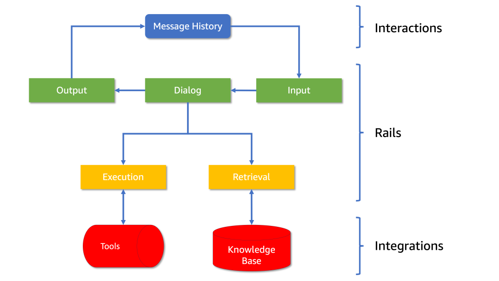
Diagram 1: The architecture of NeMo Guardrails, showing how interactions, rails and integrations are structured.
Within each rail, NeMo can understand user intent, invoke integrations when necessary, select the most appropriate response based on the intent and conversation history and generate a constrained message as a reply (see Diagram 2).
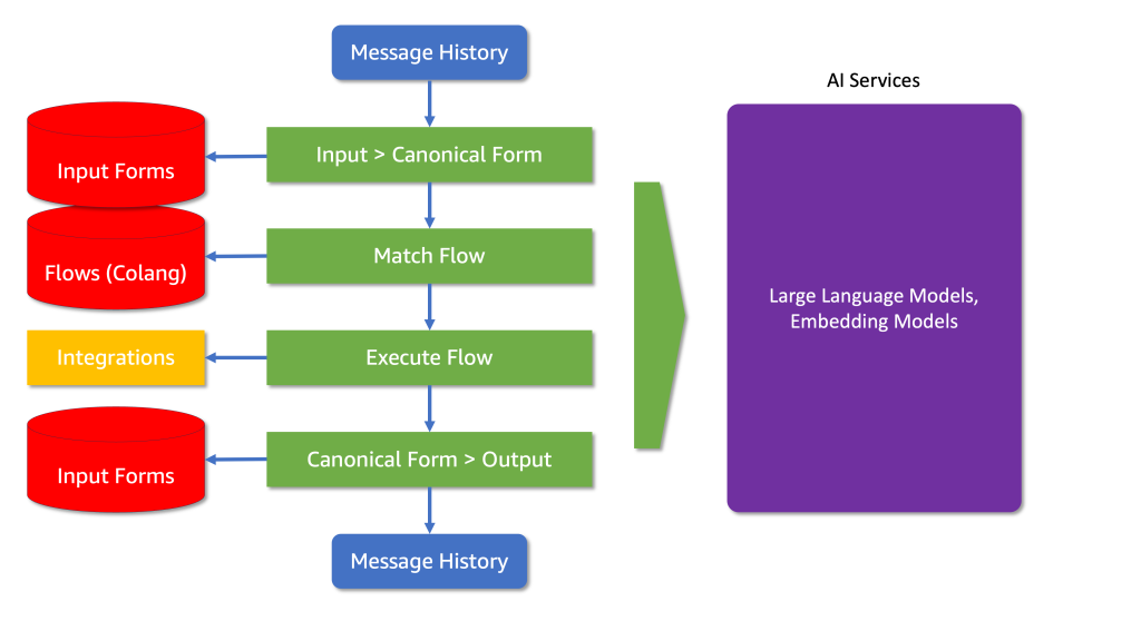
Diagram 2: The flow from input forms to the final output, including how integrations and AI services are utilized.
An Introduction to Colang
Creating a conversational AI that’s smart, engaging and operates with your use case goals in mind can be challenging. This is where NeMo Guardrails comes in. NeMo Guardrails is a toolset designed to create robust conversational agents, utilizing Colang — a modelling language specifically tailored for defining dialogue flows and guardrails. Let’s delve into how NeMo Guardrails own language can enhance your AI’s performance and provide a guided and seamless user experience.
Colang is purpose-built for simplicity and flexibility, featuring fewer constructs than typical programming languages, yet offering remarkable versatility. It leverages natural language constructs to describe dialogue interactions, making it intuitive for developers and simple to maintain.
Let’s delve into a basic Colang script to see how it works:
define user express greeting
"hello"
"hi"
"what's up?"

define bot express greeting
"Hey there!"

define bot ask how are you
"How are you doing?"

define flow greeting
user express greeting
bot express greeting
bot ask how are you
In this script, we see the three fundamental types of blocks in Colang:
- User Message Blocks (define user …): These define possible user inputs.
- Bot Message Blocks (define bot …): These specify the bot’s responses.
- Flow Blocks (define flow …): These describe the sequence of interactions.
In the example above, we defined a simple dialogue flow where a user expresses gratitude, and the bot responds with a welcoming message. This straightforward approach allows developers to construct intricate conversational pathways that uses the examples given to route the conversation toward the desired responses.
Integrating Llama 3.1 and NeMo Guardrails on SageMaker JumpStart
For this post, we’ll use Llama 3.1 8B instruct model from Meta, a recent model that strikes excellent balance between size, inference cost and conversational capabilities. We will launch it via Amazon SageMaker JumpStart, which provides access to numerous foundation models from providers such as Meta, Cohere, Hugging Face, Anthropic and more.
By leveraging SageMaker JumpStart, you can quickly evaluate and select suitable foundation models based on quality, alignment and reasoning metrics. The selected models can then be further fine-tuned on your data to better match your specific use case needs. On top of ample model choice, the additional benefit is that it enables your data to remain within your Amazon VPC during both inference and fine-tuning.
When integrating models from SageMaker JumpStart with NeMo Guardrails, the direct interaction with the SageMaker inference API requires some customization, which we will explore below.
Creating an Adapter for NeMo Guardrails
To verify compatibility, we need to create an adapter to make sure that requests and responses match the format expected by NeMo Guardrails. Although NeMo Guardrails provides a SagemakerEndpoint wrapper class, it requires some customization to handle the Llama 3.1 model API exposed by SageMaker JumpStart properly.
Below, you will find an implementation of a NeMo-compatible class that arranges the parameters required to call our SageMaker endpoint:
class ContentHandler(LLMContentHandler):
    content_type = 'application/json'
    accepts = 'application/json'

    def transform_input(self, prompt: str, model_kwargs=None):
        if model_kwargs is None:
            model_kwargs = {}

        # Ensure the 'stop' parameter is set
        model_kwargs.setdefault('stop', ['<|eot_id|>'])

        input_data = {
            'inputs': prompt,
            'parameters': model_kwargs
        }
        return json.dumps(input_data).encode("utf-8")

    def transform_output(self, output):
        output_data = json.loads(output.read().decode("utf-8"))
        return output_data.get("generated_text", f"Error: {output_data.get('error', 'Unknown error')}")

class CustomSagemakerEndpoint(SagemakerEndpoint):
    content_handler = ContentHandler()
    endpoint_name = llm_predictor.endpoint_name
    region_name = llm_predictor.sagemaker_session.boto_region_name
Structuring the Prompt for Llama 3.1
The Llama 3.1 model from Meta requires prompts to follow a specific structure, including special tokens like </s> and {role} to define parts of the conversation. When invoking the model through NeMo Guardrails, you must make sure that the prompts are formatted correctly.
To achieve seamless integration, you can modify the prompt.yaml file. Here’s an example:
prompts:
  - prompt: "<|endoftext|>{role}: {user_message}<|endoftext|>{role}: {assistant_response}"
For more details on formatting input text for Llama models, you can explore these resources:
Creating an AI Assistant
In our task to create an intelligent and responsible AI assistant for AnyCompany Pet Supplies, we’re leveraging NeMo Guardrails to build a conversational AI chatbot that can understand customer needs, provide product recommendations, and guide users through the purchase process. Here’s how we implement this.
At the heart of NeMo Guardrails are two key concepts: flows and intents. These work together to create a structured, responsive, and context-aware conversational AI.
Flows in NeMo Guardrails
Flows define the conversation structure and guide the AI’s responses. They are sequences of actions that the AI should follow in specific scenarios. For example:
define flow unrelated question
  user ask unrelated question
  bot refuse unrelated question

define flow help user with pets
  user ask about pets
  bot answer question
These flows outline how the AI should respond in different situations. When a user asks about pets, the chatbot will provide an answer. When faced with an unrelated question, it will politely refuse to answer.
Intent Capturing and Flow Selection
The process of choosing which flow to follow begins with capturing the user intent. NeMo Guardrails uses a multi-faceted approach to understand user intent:
- Pattern Matching: The system first looks for predefined patterns that correspond to specific intents:
define user ask about pets
  "What are the best shampoos for dogs?"
  "How frequently should I take my puppy on walks?"
  "How do I train my cat?"

define user ask unrelated question
  "Can you help me with my travel plans?"
  "What's the weather like today?"
  "Can you provide me with some investment advice?"
- Dynamic Intent Recognition: After selecting the most likely candidates, NeMo uses a sophisticated intent recognition system defined in the
prompts.yml file to narrow down the intent:
- task: generate_user_intent
  content: |-
    <|begin_of_text|><|start_header_id|>system<|end_header_id|>
    You are a helpful AI assistant specialised in pet products.<|eot_id|>
    <|start_header_id|>user<|end_header_id|>
    """
    {{ general_instructions }}
    """

    # This is an example how a conversation between a user and the bot can go:
    {{ sample_conversation }}
    # The previous conversation was just an example

    # This is the current conversation between the user and the bot:
    Assistant: Hello
    {{ history | user_assistant_sequence }}

    # Choose the user current intent from this list: {{ potential_user_intents }}

    Ignore the user question. The assistant task is to choose an intent from this list. The last messages are more important for defining the current intent.
    Write only one of: {{ potential_user_intents }}
    <|eot_id|><|start_header_id|>assistant<|end_header_id|>
  stop:
    - "<|eot_id|>"
This prompt is designed to guide the chatbot in determining the user’s intent. Let’s break it down:
- Context Setting: The prompt begins by defining the AI’s role as a pet product specialist. This focuses the chatbot’s attention on pet-related queries.
- General Instructions: The
{{ general_instructions }} variable contains overall guidelines for the chatbot’s behavior, as defined in our config.yml.
- Example Conversation: The
{{ sample_conversation }} provides a model of how interactions should flow, giving the chatbot context for understanding user intents.
- Current Conversation: The
{{ history | user_assistant_sequence }} variable includes the actual conversation history, allowing the chatbot to consider the context of the current interaction.
- Intent Selection: The chatbot is instructed to choose from a predefined list of intents
{{ potential_user_intents }}. This constrains the chatbot to a set of known intents, ensuring consistency and predictability in intent recognition.
- Recency Bias: The prompt specifically mentions that “the last messages are more important for defining the current intent.” This instructs the chatbot to prioritize recent context, which is often most relevant to the current intent.
- Single Intent Output: The chatbot is instructed to “Write only one of:
{{ potential_user_intents }}“. This provides a clear, unambiguous intent selection.
In Practice:
Here’s how this process works in practice (see Diagram 3):
- When a user sends a message, NeMo Guardrails initiates the intent recognition task.
- The chatbot reviews the conversation history, focusing on the most recent messages.
- It matches the user’s input against a list of predefined intents.
- The chatbot selects the most suitable intent based on this analysis.
- The identified intent determines the corresponding flow to guide the conversation.
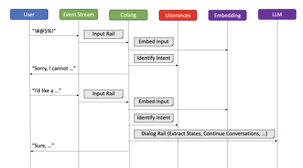
Diagram 3: Two example conversation flows, one denied by the input rails, one allowed to the dialog rail where the LLM picks up the conversation.
For example, if a user asks, “What’s the best food for a kitten?”, the chatbot might classify this as a “product_inquiry” intent. This intent would then activate a flow designed to recommend pet food products.
While this structured approach to intent recognition makes sure that the chatbot’s responses are focused and relevant to the user’s needs, it may introduce latency due to the need to process and analyze conversation history and intent in real-time. Each step, from intent recognition to flow selection, involves computational processing, which can impact the response time, especially in more complex interactions. Finding the right balance between flexibility, control, and real-time processing is crucial for creating an effective and reliable conversational AI system.
Implement Sophisticate Conversation Flows
In our earlier discussion about Colang, we examined its core structure and its role in crafting conversational flows. Now, we will delve into one of Colang’s standout features: the ability to utilize variables to capture and process user input. This functionality enables us to construct conversational agents that are not only more dynamic but also highly responsive, tailoring their interactions based on precise user data.
Continuing with our practical example of developing a pet store assistant chatbot:
define flow answer about pet products
  user express pet products needs

  $pet_type = ...

  if $pet_type == "not available"
    bot need clarification
  else
    if $pet_type == "dog":
      bot say "Depending on your dog's coat type, different grooming tools like deshedding brushes or mitts might be useful."
    else if $pet_type == "bird"
      bot say "For birds, it's crucial to use non-toxic cleaning products and sprays to maintain healthy feathers. I recommend looking for products specifically labeled for avian use."
    else
      bot say "For cats, especially those with long hair, a good brushing routine with a wire or bristle brush can help prevent mats and keep their coat healthy."
In the provided example above, we encounter the line:
$pet_type = ...
The ellipsis (...) serves as a placeholder in Colang, signaling where data extraction or inference is to be performed. This notation does not represent executable code but rather suggests that some form of logic or natural language processing should be applied at this stage.
More specifically, the use of an ellipsis here implies that the system is expected to:
- Analyze the user’s input previously captured under “user express pet products needs.”
- Determine or infer the type of pet being discussed.
- Store this information in the $pet_type variable.
The comment accompanying this line sheds more light on the intended data extraction process:
#extract the specific pet type at very high level if available, like dog, cat, bird. Make sure you still class things like puppy as "dog", kitty as "cat", etc. if available or "not available" if none apply
This directive indicates that the extraction should:
- Recognize the pet type at a high level (dog, cat, bird).
- Classify common variations (e.g., “puppy” as “dog”).
- Default to “not available” if no clear pet type is identified.
Returning to our initial code snippet, we use the $pet_type variable to customize responses, enabling the bot to offer specific advice based on whether the user has a dog, bird, or cat.
Next, we will expand on this example to integrate a Retrieval Augmented Generation (RAG) workflow, enhancing our assistant’s capabilities to recommend specific products tailored to the user’s inputs.
Bring Your Data into the Conversation
Incorporating advanced AI capabilities using a model like the Llama 3.1 8B instruct model requires more than just managing the tone and flow of conversations; it necessitates controlling the data the model accesses to respond to user queries. A common technique to achieve this is Retrieval Augmented Generation (RAG). This method involves searching a semantic database for content relevant to a user’s request and incorporating those findings into the model’s response context.
The typical approach uses an embedding model, which converts a sentence into a semantic numeric representation—referred to as a vector. These vectors are then stored in a vector database designed to efficiently search and retrieve closely related semantic information. For more information on this topic, please refer to Getting started with Amazon Titan Text Embeddings in Amazon Bedrock.
NeMo Guardrails simplifies this process: developers can store relevant content in a designated ‘kb’ folder. NeMo automatically reads this data, applies its internal embedding model and stores the vectors in an “Annoy” index, which functions as an in-memory vector database. However, this method might not scale well for extensive data sets typical in e-commerce environments. To address scalability, here are two solutions:
- Custom Adapter or Connector: Implement your own extension of the
EmbeddingsIndex base class. This allows you to customize storage, search and data embedding processes according to your specific requirements, whether local or remote. This integration makes sure that that relevant information remains in the conversational context throughout the user interaction, though it does not allow for precise control over when or how the information is used. For example:
class CustomVectorDatbaseConnector(EmbeddingsIndex):
    @property
    def embedding_size(self):
        return 768

    async def add_item(self, item: IndexItem):
        """Adds a new item to the index."""
        pass  # Implementation needed

    async def add_items(self, items: List[IndexItem]):
        """Adds multiple items to the index."""
        pass  # Implementation needed

    async def search(self, text: str, max_results: int) -> List[IndexItem]:
        """
        Searches for items in the index that are most similar to the provided text.
        """
- Retrieval Augmented Generation via Function Call: Define a function that handles the retrieval process using your preferred provider and technique. This function can directly update the conversational context with relevant data, ensuring that the AI can consider this information in its responses. For example:
async def rag(context: dict, llm: BaseLLM, search: str) -> ActionResult:
   """ retrieval component of a retrieval augmented generation function
       you can directly manipulate the NeMo's in-context knowledge here using:
       context_updates = {"relevant_chunks": json.dumps(data)}
   """
   return "true"
In the conversation rail’s flow, use variables and function calls to precisely manage searches and the integration of results:
#describe the characteristics of a product that would satisfy the user
$product_characteristics = ...
$is_success = execute rag(search=$product_characteristics)
These methods offer different levels of flexibility and control, making them suitable for various applications depending on the complexity of your system. In the next section, we will see how these techniques are applied in a more complex scenario to further enhance the capabilities of our AI assistant.
Complete Example with Variables, Retrievers and Conversation Flows
Scenario Overview
Let’s explore a complex implementation scenario with NeMo Guardrails interacting with multiple tools to drive specific business outcomes. We’ll keep the focus on the pet store e-commerce site that is being upgraded with a conversational sales agent. This agent is integrated directly into the search field at the top of the page. For instance, when a user searches for “double coat shampoo,” the results page displays several products and a chat window automatically engages the user by processing the search terms.
Detailed Conversation Flow
As the user interaction begins, the AI processes the input from the search field:
define flow answer about pet products
  user express pet products needs
  #extract the specific pet type at very high level if available, like dog, cat, bird if available or "pet" if none apply
  $pet_type = ...
  #extract the specific breed of the pet if available or "not available" if none apply
  $pet_breed = ...
  if $pet_breed == "not available"
    bot ask informations about the pet breed
Output: "Would you be able to share the type of your dog breed?"
This initiates the engine’s recognition of the user’s intent to inquire about pet products. Here, the chatbot uses variables to try and extract the type and breed of the pet. If the breed isn’t immediately available from the input, the bot requests further clarification.
Retrieval and Response Generation
If the user responds with the breed (e.g., “It’s a Labradoodle”), the chatbot proceeds to tailor its search for relevant products:
else:
    #describe the characteristics of a product that would satisfy the user
    $product_characteristics = ...
    #call our previously defined retrieval function
    $results = execute rag(search=$product_characteristics)
    #write a text message describing in a list all the products in the addional context writing their name and their ASIN number
    #and any features that relate to the user needs, offering to put one in the cart, in a single paragraph
    $product_message = ...
    bot $product_message
Output: We found several shampoos for Labradoodles: [Product List]. Would you like to add any of these to your cart?
The chatbot uses the extracted variables to refine product search criteria, then retrieves relevant items using an embedded retrieval function. It formats this information into a user-friendly message, listing available products and offering further actions.
Advancing the Sale
If the user expresses a desire to purchase a product (“I’d like to buy the second option from the list”), the chatbot transitions to processing the order:
define flow user wants product
  user express intent to buy
  #the value must be the user city of residence or "unknown"
  $user_city = ...
  #the value must be the user full street address or "unknown"
  $user_address_street = ...
  if $user_city == "unknown"
    if $user_address_street == "unknown"
      bot ask address
Output: "Great choice! To finalize your order, could you please provide your full shipping address?"
At this point, we wouldn’t have the shipping information so the bot ask for it. However, if this was a known customer, the data could be injected into the conversation from other sources. For example, if the user is authenticated and has made previous orders, their shipping address can be retrieved from the user profile database and automatically populated within the conversation flow. Then the model would just have asked for confirmation about the purchase, skipping the part about asking for shipping information.
Completing the Sale
Once our variables are filled and we have enough information to process the order, we can transition the conversation naturally into a sales motion and have the bot finalize the order:
else:
  #the value must be asin of the product the user intend to buy
  $product_asin = ...
  $cart = execute add_order(city=$user_city, street=$user_address_street, product=$product_asin)
  bot $cart
Output: "Success"
In this example, we’ve implemented a mock function called add_order to simulate a backend service call. This function verifies the address and places the chosen product into the user’s session cart. You can capture the return string from this function on the client side and take further action, for instance, if it indicates ‘Success,’ you can then run some JavaScript to display the filled cart to the user. This will show the cart with the item, pre-entered shipping details and a ready checkout button within the user interface, closing the sales loop experience for the user and tying together the conversational interface with the shopping cart and purchasing flow.
Maintaining Conversation Integrity
During this interaction, the NeMo Guardrails framework maintains the conversation within the boundaries set by the Colang configuration. For example, if the user deviates with a question such as ‘What’s the weather like today?’, NeMo Guardrails will classify this as part of a refusal flow and outside the relevant topics of ordering pet supplies. It will then tactfully declines to address the unrelated query and steers the discussion back towards selecting and ordering products, replying with a standard response like, ‘I’m afraid I can’t help with weather information, but let’s continue with your pet supplies order.’ as defined in Colang.
Clean Up
When using Amazon SageMaker JumpStart you’re deploying the selected models using on-demand GPU instances managed by Amazon SageMaker. These instances are billed per second and it’s important to optimize your costs by turning off the endpoint when not needed.
To clean up your resources, please ensure that you run the clean up cells in the three notebooks that you used. Make sure you delete the appropriate model and endpoints by executing similar cells:
llm_model.delete_model()
llm_predictor.delete_predictor()
Please note that in the third notebook, you additionally need to delete the embedding endpoints:
embedding_model.delete_model()
embedding_predictor.delete_predictor()
Additionally, you can make sure that you have deleted the appropriate resources manually by completing the following steps:
- Delete the model artifacts:
- On the Amazon SageMaker console, choose Models under Inference in the navigation pane.
- Please ensure you do not have
llm-model and embedding-model artifacts.
- To delete these artifacts, choose the appropriate models and click Delete under Actions dropdown menu.
- Delete endpoint configurations:
- On the Amazon SageMaker console, choose Endpoint configuration under Inference in the navigation pane.
- Please ensure you do not have
llm-model and embedding-model endpoint configuration.
- To delete these configurations, choose the appropriate endpoint configurations and click Delete under Actions dropdown menu.
- Delete the endpoints:
- On the Amazon SageMaker console, choose Endpoints under Inference in the navigation pane.
- Please ensure you do not have
llm-model and embedding-model endpoints running.
- To delete these endpoints, choose the appropriate model endpoint names and click Delete under Actions dropdown menu.
Best Practices and Considerations
When integrating NeMo Guardrails with SageMaker JumpStart, it’s important to consider AI governance frameworks and security best practices to ensure responsible AI deployment. While this blog focuses on showcasing the core functionality and capabilities of NeMo Guardrails, security aspects are beyond its scope.
For further guidance, please explore:
Conclusion
Integrating NeMo Guardrails with Large Language Models (LLMs) is a powerful step forward in deploying AI in customer-facing applications. The example of AnyCompany Pet Supplies illustrates how these technologies can enhance customer interactions while handling refusal and guiding the conversation toward the implemented outcomes. Looking forward, maintaining this balance of innovation and responsibility will be key to realizing the full potential of AI in various industries. This journey towards ethical AI deployment is crucial for building sustainable, trust-based relationships with customers and shaping a future where technology aligns seamlessly with human values.
Next Steps
You can find the examples used within this article via this link.
We encourage you to explore and implement NeMo Guardrails to enhance your own conversational AI solutions. By leveraging the guardrails and techniques demonstrated in this post, you can quickly constraint LLMs to drive tailored and effective results for your use case.
About the Authors
 Georgi Botsihhin is a Startup Solutions Architect at Amazon Web Services (AWS), based in the United Kingdom. He helps customers design and optimize applications on AWS, with a strong interest in AI/ML technology. Georgi is part of the Machine Learning Technical Field Community (TFC) at AWS. In his free time, he enjoys staying active through sports and taking long walks with his dog.
 Lorenzo Boccaccia is a Startup Solutions Architect at Amazon Web Services (AWS), based in Spain. He helps startups in creating cost-effective, scalable solutions for their workloads running on AWS, with a focus on containers and EKS. Lorenzo is passionate about Generative AI and is is a certified AWS Solutions Architect Professional, Machine Learning Specialist and part of the Containers TFC. In his free time, he can be found online taking part sim racing leagues.
Read More

 Tim Krause is Lead MLOps Architect at CONXAI. He takes care of all activities when AI meets infrastructure. He joined the company with previous Platform, Kubernetes, DevOps, and Big Data knowledge and was training LLMs from scratch.
 Mehdi Yosofie is a Solutions Architect at AWS, working with startup customers, and leveraging his expertise to help startup customers design their workloads on AWS.


 Olivier Vigneresse is a Solutions Architect at AWS. Based in England, he primarily works with SMB Media an&d Entertainment customers. With a background in security and networking, Olivier helps customers achieve success on their cloud journey by providing architectural guidance and best practices; he is also passionate about helping them bring value with Machine Learning and Generative AI use-cases.
 Daniel Goller is a Lead R&D Developer at Untold Studios with a focus on cloud infrastructure and emerging technologies. After earning his PhD in Germany, where he collaborated with industry leaders like BMW and Audi, he has spent the past decade implementing software solutions, with a particular emphasis on cloud technology in recent years. At Untold Studios, he leads infrastructure optimisation and AI/ML initiatives, leveraging his technical expertise and background in research to drive innovation in the Media & Entertainment space.
 Max Barnett is an Account Manager at AWS who specialises in accelerating the cloud journey of Media & Entertainment customers. He has been helping customers at AWS for the past 4.5 years. Max has been particularly involved with customers in the visual effect space, guiding them as they explore generative AI.

 Satveer Khurpa is a Sr. WW Specialist Solutions Architect, Bedrock at Amazon Web Services. In this role, he uses his expertise in cloud-based architectures to develop innovative generative AI solutions for clients across diverse industries. Satveer’s deep understanding of generative AI technologies allows him to design scalable, secure, and responsible applications that unlock new business opportunities and drive tangible value.
 Adewale Akinfaderin is a Sr. Data Scientist–Generative AI, Amazon Bedrock, where he contributes to cutting edge innovations in foundational models and generative AI applications at AWS. His expertise is in reproducible and end-to-end AI/ML methods, practical implementations, and helping global customers formulate and develop scalable solutions to interdisciplinary problems. He has two graduate degrees in physics and a doctorate in engineering.
 Antonio Rodriguez is a Principal Generative AI Specialist Solutions Architect at Amazon Web Services. He helps companies of all sizes solve their challenges, embrace innovation, and create new business opportunities with Amazon Bedrock. Apart from work, he loves to spend time with his family and play sports with his friends.


 Deepti Tirumala is a Senior Solutions Architect at Amazon Web Services, specializing in Machine Learning and Generative AI technologies. With a passion for helping customers advance their AWS journey, she works closely with organizations to architect scalable, secure, and cost-effective solutions that leverage the latest innovations in these areas.
 James Wu is a Senior AI/ML Specialist Solution Architect at AWS. helping customers design and build AI/ML solutions. James’s work covers a wide range of ML use cases, with a primary interest in computer vision, deep learning, and scaling ML across the enterprise. Prior to joining AWS, James was an architect, developer, and technology leader for over 10 years, including 6 years in engineering and 4 years in marketing & advertising industries.
 Diwakar Bansal is a Principal GenAI Specialist focused on business development and go-to- market for GenAI and Machine Learning accelerated computing services. Diwakar has led product definition, global business development, and marketing of technology products in the fields of IOT, Edge Computing, and Autonomous Driving focusing on bringing AI and Machine learning to these domains. Diwakar is passionate about public speaking and thought leadership in the Cloud and GenAI space.


 Javier Beltrán is a Senior Machine Learning Engineer at Aetion. His career has focused on natural language processing, and he has experience applying machine learning solutions to various domains, from healthcare to social media.
 Ornela Xhelili is a Staff Machine Learning Architect at Aetion. Ornela specializes in natural language processing, predictive analytics, and MLOps, and holds a Master’s of Science in Statistics. Ornela has spent the past 8 years building AI/ML products for tech startups across various domains, including healthcare, finance, analytics, and ecommerce.
 Prasidh Chhabri is a Product Manager at Aetion, leading the Aetion Evidence Platform, core analytics, and AI/ML capabilities. He has extensive experience building quantitative and statistical methods to solve problems in human health.
 Mikhail Vaynshteyn is a Solutions Architect with Amazon Web Services. Mikhail works with healthcare life sciences customers and specializes in data analytics services. Mikhail has more than 20 years of industry experience covering a wide range of technologies and sectors.


 Purna Sanyal is GenAI Specialist Solution Architect at AWS, helping customers to solve their business problems with successful adoption of cloud native architecture and digital transformation. He has specialization in data strategy, machine learning and Generative AI. He is passionate about building large-scale ML systems that can serve global users with optimal performance.
 Andrés Vélez Echeveri is a Staff Data Scientist and Machine Learning Engineer at OfferUp, focused on enhancing the search experience by optimizing retrieval and ranking components within a recommendation system. He has a specialization in machine learning and generative AI. He is passionate about creating scalable AI systems that drive innovation and user impact.
 Sean Azlin is a Principal Software Development Engineer at OfferUp, focused on leveraging technology to accelerate innovation, decrease time-to-market, and empower others to succeed and thrive. He is highly experienced in building cloud-native distributed systems at any scale. He is particularly passionate about GenAI and its many potential applications.


 Nick Biso is a Machine Learning Engineer at AWS Professional Services. He solves complex organizational and technical challenges using data science and engineering. In addition, he builds and deploys AI/ML models on the AWS Cloud. His passion extends to his proclivity for travel and diverse cultural experiences.
 Dr. Ian Lunsford is an Aerospace Cloud Consultant at AWS Professional Services. He integrates cloud services into aerospace applications. Additionally, Ian focuses on building AI/ML solutions using AWS services.