Posts in category: Amazon AWS

In previous blog post, we described an end-to-end identity verification solution in a single AWS Region. The solution uses the Amazon Rekognition APIs DetectFaces for face detection and CompareFaces for face comparison. We think of those APIs as stateless APIs because they don’t depend on an Amazon Rekognition face collection. They’re also idempotent, meaning repeated calls with the same parameters will return the same result. They provide flexible options on passing images, either through an Amazon Simple Storage Service (Amazon S3) location or raw bytes.

In this post, we focus on Amazon Rekognition Image stateless APIs, and discuss two options of passing images and when to choose one over the other from a system architecture point of view. Then we discuss how to scale the stateless APIs to overcome some Regional limitations. When talking about scalability, we often refer to the maximum transactions per second (TPS) the solution can handle. For example, when hosting a large event that uses computer vision to detect faces or object labels, you may encounter a traffic spike, and you don’t want the system to throttle. That means you sometimes need to increase the TPS and even go beyond the Regional service quota Amazon Rekognition APIs have. This post proposes a solution to increase the stateless APIs’ TPS by using multiple Regions.

Amazon Rekognition stateless APIs

Of the Amazon Rekognition Image APIs available, CompareFaces, DetectFaces, DetectLabels, DetectModerationLabels, DetectProtectiveEquipment, DetectText, and RecognizeCelebrities are stateless. They provide both Amazon S3 and raw bytes options to pass images. For example, in the request syntax of the DetectFaces API, there are two options to pass to the Image field: Bytes or S3Object.

When using the S3Object option, a typical architecture is as follows.

This solution has the following workflow:

1. The client application accesses a webpage hosted with AWS Amplify.
2. The client application is authenticated and authorized with Amazon Cognito.
3. The client application uploads an image to an S3 bucket.
4. Amazon S3 triggers an AWS Lambda function to call Amazon Rekognition.
5. The Lambda function calls Amazon Rekognition APIs with the S3Object option.
6. The Lambda function persists the result to an Amazon DynamoDB table.

Choose the S3Object option in the following scenarios:

• The image is either a PNG or JPEG formatted file
• You deploy the whole stack in the same Region where Amazon Rekognition is available
• The Regional service quota of the Amazon Rekognition API meets your system requirement

When you don’t meet all these requirements, you should choose the Bytes option.

Use Amazon Rekognition Stateless APIs in a different Region

One example of using the Bytes option is when you want to deploy your use case in a Region where Amazon Rekognition is not generally available, for example, if you have customer presence in the South America (sa-east-1) Region. For data residency, the S3 bucket that you use to store users’ images has to be in sa-east-1, but you want to use Amazon Rekognition for your solution even though it’s not generally available in sa-east-1. One solution is to use the Bytes option to call Amazon Rekognition in a different Region where Amazon Rekognition is available, such as us-east-1. The following diagram illustrates this architecture.

After the Lambda function is triggered (Step 4), instead of calling Amazon Rekognition directly with the image’s S3 location, the function needs to retrieve the image from the S3 bucket (Step 5), then call Amazon Rekognition with the image’s raw bytes (Step 6). The following is a code snippet of the Lambda function:

rekognition_region = os.getenv("REKOGNITION_REGION")
s3 = boto3.client('s3')
rekognition = boto3.client('rekognition', region_name=rekognition_region)

def handler(event, context):
    bucket = event['Records'][0]['s3']['bucket']['name']
    key = urllib.parse.unquote_plus(
    event['Records'][0]['s3']['object']['key'], encoding='utf-8')
    s3_res = s3.get_object(Bucket=bucket, Key=key)
    rekognition_res = rekognition.detect_faces(Image={"Bytes": s3_res['Body'].read()}, Attributes=['ALL'])
    print(json.dumps(rekognition_res))

Note that the preceding code snippet works directly for JPEG or PNG formats. For other image formats, like BMP, extra image processing is needed to convert it to JPEG or PNG bytes before sending to Amazon Rekognition. The following code converts BMP to JPEG bytes:

import io
from PIL import Image

s3_res = s3.get_object(Bucket=bucket, Key=key)
bmp_img = Image.open(io.BytesIO(s3_res['Body'].read()))
buffered = io.BytesIO()
rgb_img = bmp_img.convert('RGB')
rgb_img.save(buffered, format="JPEG")
rekognition_res = rekognition.detect_faces(Image={"Bytes": buffered.getvalue()}, Attributes=['ALL'])

Scale up stateless APIs’ TPS by spreading API calls into multiple Regions

Another use case of the Bytes option is that you can scale up the stateless APIs’ TPS by spreading the API calls into multiple Regions. This way, you’re not limited by the Regional service quota of the API because you can gain additional TPS from other Regions.

In the following example, a Lambda function is created to call the Amazon Rekognition DetectLabels API with the Bytes option. To scale up the maximum TPS, you can spread the API calls into multiple Regions with weights. The maximum TPS you can achieve is calculated with: min(region_1_max_tps/region_1_weight, region_2_max_tps/region_2_weight, … region_n_max_tps/region_n_weight). The following example uses us-east-1 and us-west-2 Regions.

The code snippet to call the DetectLabels API is as follows:

region_1 = os.getenv("REKOGNITION_REGION_1")
region_2 = os.getenv("REKOGNITION_REGION_2")
region_1_traffic_percentage = int(os.getenv("REGION_1_TRAFFIC_PERCENTAGE"))

# randomly generate a number between 1, 100
random_num = random.randint(1, 100)
region = region_1 if random_num <= region_1_traffic_percentage else region_2
rekognition = boto3.client('rekognition', region_name=region)
response = rekognition.detect_labels(Image={"Bytes": image_bytes})
print(response)

Because us-east-1 and us-west-2 both have maximum 50 TPS for the Amazon Rekognition DetectFaces API, you can evenly spread the API calls with 50/50 weight by setting the environment variable REGION_1_TRAFFIC_PERCENTAGE to 50. This way, you can achieve min(50/50%, 50/50%) = 100 TPS in theory.

To validate the idea, the Lambda function is exposed as a REST API with Amazon API Gateway. Then JMeter is used to load test the API.

REGION_1_TRAFFIC_PERCENTAGE is first set to 100, this way all DetectFaces API calls are sent to us-east-1 only. In theory, the maximum TPS that can be achieved is limited by the service quota in us-east-1, which is 50 TPS. Load test on the custom API endpoint, starting with 50 concurrent threads, incrementally adding 5 threads until ProvisionedThroughputExceededException returned from Amazon Rekognition is observed.

REGION_1_TRAFFIC_PERCENTAGE is then set to 50, this way all DetectLabels API calls are evenly sent to us-east-1 and us-west-2. In theory, the maximum TPS that can be achieved is the service quota that the two Regions combine, which is 100 TPS. Start the load test again from 100 threads to find the maximum TPS.

The following table summarizes the results of the load testing.

Conclusion

Many customers are using Amazon Rekognition Image stateless APIs for various use cases, including identity verification, content moderation, media processing, and more. This post discussed the two options of passing images and how to use the raw bytes option for the following use cases:

• Amazon Rekognition Regional availability
• Customer data residency
• Scaling up Amazon Rekognition stateless APIs’ TPS

Check out how Amazon Rekognition is used in different computer vision use cases and start your innovation journey.

About the Authors

Sharon Li is a solutions architect at AWS, based in the Boston, MA area. She works with enterprise customers, helping them solve difficult problems and build on AWS. Outside of work, she likes to spend time with her family and explore local restaurants.

Vaibhav Shah is a Senior Solutions Architect with AWS and like to help his customers out with everything cloud and enable their cloud adoption journey. Outside of work, he loves traveling, exploring new places and restaurants, cooking, following sports like cricket and football, watching movies and series (Marvel fan), and adventurous activities like hiking, skydiving, and the list goes on.

Read More

The success of any machine learning (ML) pipeline depends not just on the quality of model used, but also the ability to train and iterate upon this model. One of the key ways to improve an ML model is by choosing better tunable parameters, known as hyperparameters. This is known as hyperparameter optimization (HPO). However, doing this tuning manually can often be cumbersome due to the size of the search space, sometimes involving thousands of training iterations.

This post shows how Amazon SageMaker enables you to not only bring your own model algorithm using script mode, but also use the built-in HPO algorithm. You will learn how to easily output the evaluation metric of choice to Amazon CloudWatch, from which you can extract this metric to guide the automatic HPO algorithm. You can then create an HPO tuning job that orchestrates several training jobs and associated compute resources. Upon completion, you can see the best training job according to the evaluation metric.

Solution overview

We walk through the following steps:

1. Use SageMaker script mode to bring our own model on top of an AWS-managed container.
2. Refactor our training script to print out our evaluation metric.
3. Find the metric in CloudWatch Logs.
4. Extract the metric from CloudWatch.
5. Use HPO to select the best model by tuning on this evaluation metric.
6. Monitor the HPO and find the best training job.

Prerequisites

For this walkthrough, you should have the following prerequisites:

• An AWS account.
• An Amazon Simple Storage Service (Amazon S3) bucket. For instructions on creating a bucket, see Step 1: Create your first S3 bucket.
• An AWS Identity and Access Management (IAM) role. To build and run an ML model using SageMaker, you must provide an IAM role that grants SageMaker permission to access Amazon S3 in your account to fetch the training and test datasets.
• A SageMaker notebook instance. For instructions, see Create a Notebook Instance. Attach the IAM role you created for SageMaker to this notebook instance.

Use custom algorithms on an AWS-managed container

Refer to Bring your own model with Amazon SageMaker script mode for a more detailed look at bringing a custom model into SageMaker using an AWS-managed container.

We use the MNIST dataset for this example. MNIST is a widely used dataset for handwritten digit classification, consisting of 70,000 labeled 28×28 pixel grayscale images of handwritten digits. The dataset is split into 60,000 training images and 10,000 test images, containing 10 classes (one for each digit).

1. Open your notebook instance and run the following command to downloaded the mnist.py file:

   !wget https://raw.githubusercontent.com/aws/amazon-sagemaker-examples/main/hyperparameter_tuning/pytorch_mnist/mnist.py

   Before we get and store the data, let’s create a SageMaker session. We should also specify the S3 bucket and prefix to use for training and model data. This should be within the same Region as the notebook instance, training, and hosting. The following code uses the default bucket if it already exists, or creates a new one if it doesn’t. We also must include the IAM role ARN to give training and hosting access to your data. We use get_execution_role() to get the IAM role that you created for your notebook instance.

2. Create a session with the following code:

   import sagemaker
   from sagemaker.tuner import (
   IntegerParameter,
   CategoricalParameter,
   ContinuousParameter,
   HyperparameterTuner,
   )
   session = sagemaker.Session()
   bucket = session.default_bucket()
   prefix = "sagemaker/DEMO-custom-hpo"
   role = sagemaker.get_execution_role()

3. Now let’s get the data, store it in our local folder /data, and upload it to Amazon S3:

   from torchvision.datasets import MNIST
   from torchvision import transforms
   MNIST.mirrors = ["https://sagemaker-sample-files.s3.amazonaws.com/datasets/image/MNIST/"]
   MNIST(
   "data",
   download=True,
   transform=transforms.Compose(
   [transforms.ToTensor(), transforms.Normalize((0.1307,), (0.3081,))]
   ),
   )
   inputs = session.upload_data(path="data", bucket=bucket, key_prefix=prefix)

   We can now create an estimator to set up the PyTorch training job. We don’t focus on the actual training code here (mnist.py) in great detail. Let’s look at how we can easily invoke this training script to initialize a training job.

4. In the following code, we include an entry point script called mnist.py that contains our custom training code:

   from sagemaker.pytorch import PyTorch
   estimator = PyTorch(
   entry_point="mnist.py",
   role=role,
   py_version="py3",
   framework_version="1.8.0",
   instance_count=1,
   instance_type="ml.c5.2xlarge",
   hyperparameters={"epochs": 5},
   )

5. To ensure that this training job has been configured correctly, with working training code, we can start a training job by fitting it to the data we uploaded to Amazon S3. SageMaker ensures our data is available in the local file system, so our training script can just read the data from disk:

   estimator.fit({"training": inputs})

However, we’re not creating a single training job. We use the automatic model tuning capability of SageMaker through the use of a hyperparameter tuning job. Model tuning is completely agnostic to the actual model algorithm. For more information on all the hyperparameters that you can tune, refer to Perform Automatic Model Tuning with SageMaker.

For each hyperparameter that we want to optimize, we have to define the following:

• A name
• A type (parameters can either be an integer, continuous, or categorical)
• A range of values to explore
• A scaling type (linear, logarithmic, reverse logarithmic, or auto); this lets us control how a specific parameter range will be explored

We must also define the metric we’re optimizing for. It can be any numerical value as long as it’s visible in the training log and you can pass a regular expression to extract it.

If we look at line 181 in mnist.py, we can see how we print to the logger:

logger.info(
"Test set: Average loss: {:.4f}, Accuracy: {}/{} ({:.0f}%)n".format(
test_loss, correct, len(test_loader.dataset), 100.0 * correct / len(test_loader.dataset)
)

In fact, we can see this output in the logs of the training job we just ran. By opening the log group /aws/sagemaker/TrainingJobs on the CloudWatch console, we should have a log event beginning with pytorch-training- followed by a timestamp and generated name.

The following screenshot highlights the log we’re looking for.

Let’s now start on building our hyperparameter tuning job.

6. As mentioned, we must first define some information about the hyperparameters, under the object as follows:

   hyperparameter_ranges = {
   "lr": ContinuousParameter(0.001, 0.1),
   "batch-size": CategoricalParameter([32, 64, 128, 256, 512]),
   }

   Here we defined our two hyperparameters. The learning rate (lr) is a continuous parameter (therefore a continuous value) in the range 0.001 and 0.1. The batch size (batch-size) is a categorical parameter with the preceding discrete values.

   Next, we specify the objective metric that we’d like to tune and its definition. This includes the regular expression (regex) needed to extract that metric from the CloudWatch logs of the training job that we previously saw. We also specify a descriptive name average test loss and the objective type as Minimize, so the hyperparameter tuning seeks to minimize the objective metric when searching for the best hyperparameter setting.

7. Specify the metric with the following code:

   metric_definitions = [{"Name": "average test loss", "Regex": "Test set: Average loss: ([0-9\.]+)"}]
   objective_metric_name = "average test loss"
   objective_type = "Minimize"

   Now we’re ready to create our HyperparameterTuner object. In addition to the objective metric name, type, and definition, we pass in the hyperparameter_ranges object and the estimator we previously created. We also specify the number of jobs we want to run in total, along with the number that should run in parallel. We have chosen the maximum number of jobs as 9, but you would typically opt for a much higher number (such as 50) for optimal performance.

8. Create the HyperparameterTuner object with the following code:

   tuner = HyperparameterTuner(
   estimator,
   objective_metric_name,
   hyperparameter_ranges,
   metric_definitions,
   max_jobs=9,
   max_parallel_jobs=3,
   objective_type=objective_type,
   )

Before we start the tuning job, it’s worth noting how the combinations of hyperparameters are determined. To get good results, you need to choose the right ranges to explore. By default, the Bayesian search strategy is used, described further in How Hyperparameter Tuning works.

With Bayesian optimization, hyperparameter tuning is treated as a regression problem. To solve this regression problem, it makes guesses about which hyperparameter combinations will get the best results, and runs training jobs to test these values. It uses regression to choose the next set of hyperparameter values to test. There is a clear exploit/explore trade-off that the search strategy makes here. It can choose hyperparameter values close to the combination that resulted in the best previous training job to incrementally improve performance. Or, it may choose values further away, to try and explore a new range of values that isn’t yet well understood.

You may specify other search strategies, however. The following strategies are supported in SageMaker:

• Grid search – Tries every possible combination among the range of hyperparameters that is specified.
• Random search – Tries random combinations among the range of values specified. It doesn’t depend on the results of previous training jobs, so you can run the maximum number of concurrent training jobs without affecting the performance of the tuning.
• Hyperband search – Uses both intermediate and final results of training jobs to reallocate epochs to well-utilized hyperparameter configurations, and automatically stops those that underperform.

You may also explore bringing your own algorithm, as explained in Bring your own hyperparameter optimization algorithm on Amazon SageMaker.

9. We then launch training on the tuner object itself (not the estimator), calling .fit() and passing in the S3 path to our train and test dataset:

   tuner.fit({"training": inputs})

We can then follow the progress of our tuning job on the SageMaker console, on the Hyperparameter tuning jobs page. The tuning job spins up the underlying compute resources necessary by orchestrating each individual training run and its associated compute.

Then it’s easy to see all the individual training jobs that have been completed or are in progress, along with their associated objective metric value. In the following screenshot, we can see the first batch of training jobs is complete, which contains three in total according to our specified max_parallel_jobs value of 3. Upon completion, we can find the best training job—the one that minimizes average test loss—on the Best training job tab.

Clean up

To avoid incurring future charges, delete the resources you initialized. These are the S3 bucket, IAM role, and SageMaker notebook instance.

Conclusion

In this post, we discussed how we can bring our own model into SageMaker, and then use automated hyperparameter optimization to select the best training job. We used the popular MNIST dataset to look at how we can specify a custom objective metric for which the HPO job should optimize on. By extracting this objective metric from CloudWatch, and specifying various hyperparameter values, we can easily launch and monitor the HPO job.

If you need more information, or want to see how our customers are using HPO, refer to Amazon SageMaker Automatic Model Tuning. Adapt your own model for automated hyperparameter optimization in SageMaker today.

About the author

Sam Price is a a Professional Services Consultant specializing in AI/ML and data analytics at Amazon Web Services. He works closely with public sector customers in healthcare and life sciences to solve challenging problems. When not doing this, Sam enjoys playing guitar and tennis, and seeing his favorite indie bands.

Read More

With the growth and popularity of online social platforms, people can stay more connected than ever through tools like instant messaging. However, this raises an additional concern about toxic speech, as well as cyber bullying, verbal harassment, or humiliation. Content moderation is crucial for promoting healthy online discussions and creating healthy online environments. To detect toxic language content, researchers have been developing deep learning-based natural language processing (NLP) approaches. Most recent methods employ transformer-based pre-trained language models and achieve high toxicity detection accuracy.

In real-world toxicity detection applications, toxicity filtering is mostly used in security-relevant industries like gaming platforms, where models are constantly being challenged by social engineering and adversarial attacks. As a result, directly deploying text-based NLP toxicity detection models could be problematic, and preventive measures are necessary.

Research has shown that deep neural network models don’t make accurate predictions when faced with adversarial examples. There has been a growing interest in investigating the adversarial robustness of NLP models. This has been done with a body of newly developed adversarial attacks designed to fool machine translation, question answering, and text classification systems.

In this post, we train a transformer-based toxicity language classifier using Hugging Face, test the trained model on adversarial examples, and then perform adversarial training and analyze its effect on the trained toxicity classifier.

Solution overview

Adversarial examples are intentionally perturbed inputs, aiming to mislead machine learning (ML) models towards incorrect outputs. In the following example (source: https://aclanthology.org/2020.emnlp-demos.16.pdf), by changing just the word “Perfect” to “Spotless,” the NLP model gave a completely opposite prediction.

Social engineers can use this type of characteristic of NLP models to bypass toxicity filtering systems. To make text-based toxicity prediction models more robust against deliberate adversarial attacks, the literature has developed multiple methods. In this post, we showcase one of them—adversarial training, and how it improves text toxicity prediction models’ adversarial robustness.

Adversarial training

Successful adversarial examples reveal the weakness of the target victim ML model, because the model couldn’t accurately predict the label of these adversarial examples. By retraining the model with a combination of original training data and successful adversarial examples, the retrained model will be more robust against future attacks. This process is called adversarial training.

TextAttack Python library

TextAttack is a Python library for generating adversarial examples and performing adversarial training to improve NLP models’ robustness. This library provides implementations of multiple state-of-the-art text adversarial attacks from the literature and supports a variety of models and datasets. Its code and tutorials are available on GitHub.

Dataset

The Toxic Comment Classification Challenge on Kaggle provides a large number of Wikipedia comments that have been labeled by human raters for toxic behavior. The types of toxicity are:

• toxic
• severe_toxic
• obscene
• threat
• insult
• identity_hate

In this post, we only predict the toxic column. The train set contains 159,571 instances with 144,277 non-toxic and 15,294 toxic examples, and the test set contains 63,978 instances with 57,888 non-toxic and 6,090 toxic examples. We split the test set into validation and test sets, which contain 31,989 instances each with 29,028 non-toxic and 2,961 toxic examples. The following charts illustrate our data distribution.

For the purpose of demonstration, this post randomly samples 10,000 instances for training, and 1,000 for validation and testing each, with each dataset balanced on both classes. For details, refer to our notebook.

Train a transformer-based toxic language classifier

The first step is to train a transformer-based toxic language classifier. We use the pre-trained DistilBERT language model as a base and fine-tune the model on the Jigsaw toxic comment classification training dataset.

Tokenization

Tokens are the building blocks of natural language inputs. Tokenization is a way of separating a piece of text into tokens. Tokens can take several forms, either words, characters, or subwords. In order for the models to understand the input text, a tokenizer is used to prepare the inputs for an NLP model. A few examples of tokenizing include splitting strings into subword token strings, converting token strings to IDs, and adding new tokens to the vocabulary.

In the following code, we use the pre-trained DistilBERT tokenizer to process the train and test datasets:

pretrained_model_name_or_path = "distilbert-base-uncased"
tokenizer = AutoTokenizer.from_pretrained(pretrained_model_name_or_path)

def preprocess_function(examples):
    result = tokenizer(
        examples["text"], padding="max_length", max_length=128, truncation=True
    )
    return result

train_dataset = train_dataset.map(
    preprocess_function, batched=True, load_from_cache_file=False, num_proc=num_proc
)

valid_dataset = valid_dataset.map(
    preprocess_function, batched=True, load_from_cache_file=False, num_proc=num_proc
)

test_dataset = test_dataset.map(
    preprocess_function, batched=True, load_from_cache_file=False, num_proc=num_proc
)

For each input text, the DistilBERT tokenizer outputs four features:

• text – Input text.
• labels – Output labels.
• input_ids – Indexes of input sequence tokens in a vocabulary.
• attention_mask – Mask to avoid performing attention on padding token indexes. Mask values selected are [0, 1]:
  • 1 for tokens that are not masked.
  • 0 for tokens that are masked.

Now that we have the tokenized dataset, the next step is to train the binary toxic language classifier.

Modeling

The first step is to load the base model, which is a pre-trained DistilBERT language model. The model is loaded with the Hugging Face Transformers class AutoModelForSequenceClassification:

base_model = AutoModelForSequenceClassification.from_pretrained(
    pretrained_model_name_or_path, num_labels=1
)

Then we customize the hyperparameters using class TrainingArguments. The model is trained with batch size 32 on 10 epochs with learning rate of 5e-6 and warmup steps of 500. The trained model is saved in model_dir, which was defined in the beginning of the notebook.

training_args = TrainingArguments(
    output_dir=model_dir,
    num_train_epochs=10,
    per_device_train_batch_size=32,
    per_device_eval_batch_size=64,
    warmup_steps=500,
    evaluation_strategy="epoch",
    save_strategy="epoch",
    save_total_limit=5,
    logging_dir=os.path.join(model_dir, "logs"),
    learning_rate=5e-6,
    load_best_model_at_end=True,
    metric_for_best_model="loss",
    disable_tqdm=True,
)

To evaluate the model’s performance during training, we need to provide the Trainer with an evaluation function. Here we are report accuracy, F1 scores, average precision, and AUC scores.

# compute metrics function
def compute_metrics(pred):
    targets = 1 * (pred.label_ids >= 0.5)
    outputs = 1 * (pred.predictions >= 0.5)
    accuracy = metrics.accuracy_score(targets, outputs)
    f1_score_micro = metrics.f1_score(targets, outputs, average="micro")
    f1_score_macro = metrics.f1_score(targets, outputs, average="macro")
    f1_score_weighted = metrics.f1_score(targets, outputs, average="weighted")
    ap_score_micro = metrics.average_precision_score(
        targets, pred.predictions, average="micro"
    )
    ap_score_macro = metrics.average_precision_score(
        targets, pred.predictions, average="macro"
    )
    ap_score_weighted = metrics.average_precision_score(
        targets, pred.predictions, average="weighted"
    )
    auc_score_micro = metrics.roc_auc_score(targets, pred.predictions, average="micro")
    auc_score_macro = metrics.roc_auc_score(targets, pred.predictions, average="macro")
    auc_score_weighted = metrics.roc_auc_score(
        targets, pred.predictions, average="weighted"
    )
    return {
        "accuracy": accuracy,
        "f1_score_micro": f1_score_micro,
        "f1_score_macro": f1_score_macro,
        "f1_score_weighted": f1_score_weighted,
        "ap_score_micro": ap_score_micro,
        "ap_score_macro": ap_score_macro,
        "ap_score_weighted": ap_score_weighted,
        "auc_score_micro": auc_score_micro,
        "auc_score_macro": auc_score_macro,
        "auc_score_weighted": auc_score_weighted,
    }

The Trainer class provides an API for feature-complete training in PyTorch. Let’s instantiate the Trainer by providing the base model, training arguments, training and evaluation dataset, as well as the evaluation function:

trainer = Trainer(
    model=base_model,
    args=training_args,
    train_dataset=train_dataset,
    eval_dataset=valid_dataset,
    compute_metrics=compute_metrics,
)

After the Trainer is instantiated, we can kick off the training process:

train_result = trainer.train()

When the training process is finished, we save the tokenizer and model artifacts locally:

tokenizer.save_pretrained(model_dir)
trainer.save_model(model_dir)

Evaluate the model robustness

In this section, we try to answer one question: how robust is our toxicity filtering model against text-based adversarial attacks? To answer this question, we select an attack recipe from the TextAttack library and use it to construct perturbed adversarial examples to fool our target toxicity filtering model. Each attack recipe generates text adversarial examples by transforming seed text inputs into slightly changed text samples, while making sure the seed and its perturbed text follow certain language constraints (for example, semantic preserved). If these newly generated examples trick a target model into wrong classifications, the attack is successful; otherwise, the attack fails for that seed input.

A target model’s adversarial robustness is evaluated through the Attack Success Rate (ASR) metric. ASR is defined as the ratio of successful attacks against all the attacks. The lower the ASR, the more robust a model is against adversarial attacks.

First, we define a custom model wrapper to wrap the tokenization and model prediction together. This step also makes sure the prediction outputs meet the required output formats by the TextAttack library.

class CustomModelWrapper(ModelWrapper):
    def __init__(self, model):
        self.model = model

    def __call__(self, text_input_list):
        device = self.model.device
        encoded_input = tokenizer(
            text_input_list,
            truncation=True,
            padding="max_length",
            max_length=128,
            return_tensors="pt",
        ).to(device)     
        # print(encoded_input.device)

        with torch.no_grad():
            output = self.model(**encoded_input)
        logits = output.logits
        preds = torch.sigmoid(logits)
        preds = preds.squeeze(dim=-1)
        final_preds = torch.stack((1 - preds, preds), dim=1)
        return final_preds

Now we load the trained model and create a custom model wrapper using the trained model:

trained_model = AutoModelForSequenceClassification.from_pretrained(model_dir)
trained_model = trained_model.to("cuda:0")

model_wrapper = CustomModelWrapper(trained_model)

Generate attacks

Now we need to prepare the dataset as seed for an attack recipe. Here we only use those toxic examples as seeds, because in a real-world scenario, the social engineer will mostly try to perturb toxic examples to fool a target filtering model as benign. Attacks could take time to generate; for the purpose of this post, we randomly sample 1,000 toxic training samples to attack.

We generate the adversarial examples for both test and train datasets. We use test adversarial examples for robustness evaluation and the train adversarial examples for adversarial training.

threshold = 0.5
sub_sample_to_attack = 1000
df_train_to_attack = df_train[df_train['labels']==1].sample(sub_sample_to_attack)

## We attack the toxic samples
## Goal is to perturbe toxic samples enough that the model classifies them as Non-toxic
test_dataset_to_attack = textattack.datasets.Dataset(
    [
        (x, 1)
        for x, y in zip(
            test_dataset["text"], 
            test_dataset["labels"], 
        )
        if y > threshold
    ]
)

train_dataset_to_attack = textattack.datasets.Dataset(
    [
        (x, 1)
        for x, y in zip(
            df_train_to_attack["text"],
            df_train_to_attack["labels"],
        )
        if y > threshold
    ]
)

Then we define the function to generate the attacks:

def generate_attacks(
    recipe, model_wrapper, dataset_to_attack, num_examples=-1, parallel=False
):
    print(f"The Attack Recipe is: {recipe}")
    if recipe == "textfoolerjin2019":
        attack = TextFoolerJin2019.build(model_wrapper)
    elif recipe == "a2t_yoo_2021":
        attack = A2TYoo2021.build(model_wrapper)
    elif recipe == "Pruthi2019":
        attack = Pruthi2019.build(model_wrapper)
    elif recipe == "TextBuggerLi2018":
        attack = TextBuggerLi2018.build(model_wrapper)
    elif recipe == "DeepWordBugGao2018":
        attack = DeepWordBugGao2018.build(model_wrapper)

    attack_args = textattack.AttackArgs(
        num_examples=num_examples, parallel=parallel, num_workers_per_device=5
    )  
    ## num_examples = -1 means the entire dataset
    attacker = Attacker(attack, dataset_to_attack, attack_args)
    attack_results = attacker.attack_dataset()
    return attack_results

Choose an attack recipe and generate attacks:

%%time
recipe = 'textfoolerjin2019'
test_attack_results = generate_attacks(recipe, model_wrapper, test_dataset_to_attack, num_examples=-1)
train_attack_results = generate_attacks(recipe, model_wrapper, train_dataset_to_attack, num_examples=-1)

Log the attack results into a Pandas data frame:

def log_attack_results(attack_results):
    exception_ids = []
    logger = CSVLogger(color_method="html")
    
    for i in range(len(attack_results)):
        try:
            result = attack_results[i]
            logger.log_attack_result(result)
        except:
            exception_ids.append(i)
    df_attacks = logger.df
    return df_attacks, exception_ids


df_attacks_test, test_exception_ids = log_attack_results(test_attack_results)
df_attacks_train, train_exception_ids = log_attack_results(train_attack_results)

The attack results contain original_text, perturbed_text, original_output, and perturbed_output. When the perturbed_output is the opposite of the original_output, the attack is successful.

df_attacks_test.head(2)

display(
    HTML(df_attacks_test[["original_text", "perturbed_text"]].head().to_html(escape=False))
)

The red text represents a successful attack, and the green represents a failed attack.

Evaluate the model robustness through ASR

Use the following code to evaluate the model robustness:

ASR_test = (
    df_attacks_test.result_type.value_counts()["Successful"]
    / df_attacks_test.result_type.value_counts().sum()
)

ASR_train = (
    df_attacks_train.result_type.value_counts()["Successful"]
    / df_attacks_train.result_type.value_counts().sum()
)

print(f"The Attack Success Rate of the model toward test dataset is {ASR_test*100}%")

print(f"The Attack Success Rate of the model toward train dataset is {ASR_train*100}%")

This returns the following:

The Attack Success Rate of the model toward test dataset is 52.400000000000006%
The Attack Success Rate of the model toward train dataset is 51.1%

Prepare successful attacks

With all the attack results available, we take the successful attack from the train adversarial examples and use them to retrain the model:

# Supply the original labels to the successful attacks
# Here the original labels are all 1, there are also some datasets with fractional labels between 0-1

df_attacks_train = df_attacks_train[["perturbed_text", "result_type"]].copy()
df_attacks_train["labels"] = df_train_to_attack["labels"].reset_index(drop=True)

# Clean the text
df_attacks_train["text"] = df_attacks_train["perturbed_text"].replace(
    "<font color = .{1,6}>|</font>", "", regex=True
)
df_attacks_train["text"] = df_attacks_train["text"].replace("<SPLIT>", "n", regex=True)

# Prepare data to add to the training dataset
df_succ_attacks_train = df_attacks_train.loc[
    df_attacks_train.result_type == "Successful", ["text", "labels"]
]
df_succ_attacks_train.shape, df_succ_attacks_train.head(2)

Adversarial training

In this section, we combine the successful adversarial attacks from the training data with the original training data, then train a new model on this combined dataset. This model is called the adversarial trained model.

# New Train: Original Train + Successful Attacks on Original Train

df_train_attacked = pd.concat([df_train, df_succ_attacks_train], ignore_index=True)
data_train_attacked = Dataset.from_pandas(df_train_attacked)
data_train_attacked = data_train_attacked.map(
    preprocess_function, batched=True, load_from_cache_file=False, num_proc=num_proc
)

training_args_AT = TrainingArguments(
    output_dir=model_dir_AT,
    num_train_epochs=10,
    per_device_train_batch_size=32,
    per_device_eval_batch_size=64,
    warmup_steps=500,
    evaluation_strategy="epoch",
    save_strategy="epoch",
    save_total_limit=5,
    logging_dir=os.path.join(model_dir, "logs"),
    learning_rate=5e-6,
    load_best_model_at_end=True,
    metric_for_best_model="loss",
    disable_tqdm=True,
)

trainer_AT = Trainer(
    model=base_model,
    args=training_args_AT,
    train_dataset=data_train_attacked,
    eval_dataset=valid_dataset,
    compute_metrics=compute_metrics
)

trainer_AT.train()

Save the adversarial trained model to local directory model_dir_AT:

tokenizer.save_pretrained(model_dir_AT)
trainer_AT.save_model(model_dir_AT)

Evaluate the robustness of the adversarial trained model

Now the model is adversarially trained, we want to see how the model robustness changes accordingly:

trained_model_AT = AutoModelForSequenceClassification.from_pretrained(model_dir_AT)
trained_model_AT = trained_model_AT.to("cuda:0")
trained_model_AT.device

model_wrapper_AT = CustomModelWrapper(trained_model_AT)
test_attack_results_AT = generate_attacks(recipe, model_wrapper_AT, test_dataset_to_attack, num_examples=-1)
df_attacks_AT_test, AT_test_exception_ids = log_attack_results(test_attack_results_AT)

ASR_AT_test = (
    df_attacks_AT_test.result_type.value_counts()["Successful"]
    / df_attacks_AT_test.result_type.value_counts().sum()
)

print(f"The Attack Success Rate of the model is {ASR_AT_test*100}%")

The preceding code returns the following results:

The Attack Success Rate of the model is 19.8%

Compare the robustness of the original model and the adversarial trained model:

print(
    f"The ASR of the Adversarial Trained model has a {(ASR_test - ASR_AT_test)/ASR_test*100}% decrease compare with the original model. This proves that the Adversarial Training improves the model's robustness against the attacks."
)

This returns the following:

The ASR of the Adversarial Trained model has a 62.213740458015266% decrease
compare with the original model. This proves that the Adversarial Training
improves the model's robustness against the attacks.

So far, we have trained a DistilBERT-based binary toxicity language classifier, tested its robustness against adversarial text attacks, performed adversarial training to obtain a new toxicity language classifier, and tested the new model’s robustness against adversarial text attacks.

We observe that the adversarial trained model has a lower ASR, with an 62.21% decrease using the original model ASR as the benchmark. This indicates that the model is more robust against certain adversarial attacks.

Model performance evaluation

Besides model robustness, we’re also interested in learning how a model predicts on clean samples after it’s adversarially trained. In the following code, we use batch prediction mode to speed up the evaluation process:

def batch_predict(model_wrapper, text_list, batch_size=64):
    """This function performs batch prediction for given model nad text list"""
    predictions = []
    for i in tqdm(range(0, len(text_list), batch_size)):
       batch = text_list[i : i + batch_size]
       model_predictions = model_wrapper(batch)[:, 1]
       model_predictions = model_predictions.cpu().numpy()
       predictions.append(model_predictions)
       predictions = np.concatenate(predictions, axis=0)
    return predictions

Evaluate the original model

We use the following code to evaluate the original model:

test_text_list = df_test.text.to_list()

model_predictions = batch_predict(model_wrapper, test_text_list, batch_size=64)

y_true_prob = np.array(df_test["labels"])
y_true = [0 if x < 0.5 else 1 for x in y_true_prob]

threshold = 0.5
y_pred_prob = model_predictions.flatten()
y_pred = [0 if x < threshold else 1 for x in y_pred_prob]

fig, ax = plt.subplots(figsize=(10, 10))
conf_matrix = confusion_matrix(y_true, y_pred)
ConfusionMatrixDisplay(conf_matrix).plot(ax=ax)
print(classification_report(y_true, y_pred))

The following figures summarize our findings.

Evaluate the adversarial trained model

Use the following code to evaluate the adversarial trained model:

model_predictions_AT = batch_predict(model_wrapper_AT, test_text_list, batch_size=64)

y_pred_prob_AT = model_predictions_AT.flatten()
y_pred_AT = [0 if x < threshold else 1 for x in y_pred_prob_AT]

fig, ax = plt.subplots(figsize=(10, 10))
conf_matrix = confusion_matrix(y_true, y_pred_AT)
ConfusionMatrixDisplay(conf_matrix).plot(ax=ax)
print(classification_report(y_true, y_pred_AT))

The following figures summarize our findings.

We observe that the adversarial trained model tended to predict more examples as toxic (801 predicted as 1) compared with the original model (763 predicted as 1), which leads to an increase in recall of the toxic class and precision of the non-toxic class, and a drop in precision of the toxic class and recall of the non-toxic class. This might due to the fact that more of the toxic class is seen in the adversarial training process.

Summary

As part of content moderation, toxicity language classifiers are used to filter toxic content and create healthier online environments. Real-world deployment of toxicity filtering models calls for not only high prediction performance, but also for being robust against social engineering, like adversarial attacks. This post provides a step-by-step process from training a toxicity language classifier to improve its robustness with adversarial training. We show that adversarial training can help a model become more robust against attacks while maintaining high model performance. For more information about this up-and-coming topic, we encourage you to explore and test our script on your own. You can access the notebook in this post from the AWS Examples GitHub repo.

Hugging Face and AWS announced a partnership earlier in 2022 that makes it even easier to train Hugging Face models on SageMaker. This functionality is available through the development of Hugging Face AWS DLCs. These containers include the Hugging Face Transformers, Tokenizers, and Datasets libraries, which allow us to use these resources for training and inference jobs. For a list of the available DLC images, see Available Deep Learning Containers Images. They are maintained and regularly updated with security patches.

You can find many examples of how to train Hugging Face models with these DLCs in the following GitHub repo.

AWS offers pre-trained AWS AI services that can be integrated into applications using API calls and require no ML experience. For example, Amazon Comprehend can perform NLP tasks such as custom entity recognition, sentiment analysis, key phrase extraction, topic modeling, and more to gather insights from text. It can perform text analysis on a wide variety of languages for its various features.

References

• Toxicity detection sensitive to conversational context
• Toxic Speech Detection
• Toxicity Detection in online Georgian discussion
• Toxicity detection sensitive to conversational context
• Toxicity Detection: Does Context Really Matter?
• Hugging Face Trainer class
• Hugging Face Glossary
• Intriguing properties of neural networks

About the Authors

Yi Xiang is a Data Scientist II at the Amazon Machine Learning Solutions Lab, where she helps AWS customers across different industries accelerate their AI and cloud adoption.

Yanjun Qi is a Principal Applied Scientist at the Amazon Machine Learning Solution Lab. She innovates and applies machine learning to help AWS customers speed up their AI and cloud adoption.

Read More

Globally, there has been an accelerated shift toward frictionless digital user experiences. Whether it’s registering at a website, transacting online, or simply logging in to your bank account, organizations are actively trying to reduce the friction their customers experience while at the same time enhance their security, compliance, and fraud prevention measures. The shift toward frictionless user experiences has given rise to face-based biometric identity verification solutions aimed at answering the question “How do you verify a person in the digital world?”

There are two key advantages of facial biometrics when it comes to questions of identification and authentication. First, it’s a convenient technology for users: there is no need to remember a password, deal with multi-factor challenges, click verification links, or solve CAPTCHA puzzles. Secondly, a high level of security is achieved: identification and authentication on the basis of facial-biometrics is secure and less susceptible to fraud and attacks.

In this post, we dive into the two primary use cases of identity verification: onboarding and authentication. Then we dive into the two key metrics used to evaluate a biometric system’s accuracy: the false match rate (also known as false acceptance rate) and false non-match rate (also known as false rejection rate). These two measures are widely used by organizations to evaluate accuracy and error rate of biometric systems. Finally, we discuss a framework and best practices for performing an evaluation of an identity verification service.

Refer to the accompanying Jupyter notebook that walks through all the steps mentioned in this post.

Use cases: Onboarding and Authentication

There are two primary use cases for biometric solutions: user onboarding (often referred to as verification) and authentication (often referred to as identification). Onboarding entails one-to-one matching of faces between two images, for example comparing a selfie to a trusted identification document like a driver’s license or passport. Authentication, on the other hand, entails one-to-many search of a face against a stored collection of faces, for example searching a collection of employee faces to see if an employee is authorized access to a particular floor in a building.

Accuracy performance of onboarding and authentication use cases is measured by the false positive and false negative errors that the biometric solution can make. A similarity score (ranging from 0% meaning no match to 100% meaning a perfect match) is used to make the determination of a match or a non-match decision. A false positive occurs when the solution considers images of two different individuals to be the same person. A false negative, on the other hand, means that the solution considered two images of the same person to be different.

Onboarding: One-to-one verification

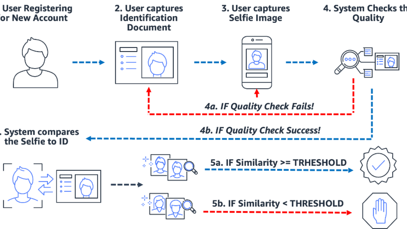
Biometric-based onboarding processes both simplify and secure the process. Most importantly, it sets the organization and customer up for a near-frictionless onboarding experience. To do this, users are simply required to present an image of some form of trusted identification document containing the user’s face (such as driver’s license or passport) as well as take a selfie image during the onboarding process. After the system has these two images, it simply compares the faces within the two images. When the similarity is greater than a specified threshold, then you have a match; otherwise, you have a non-match. The following diagram outlines the process.

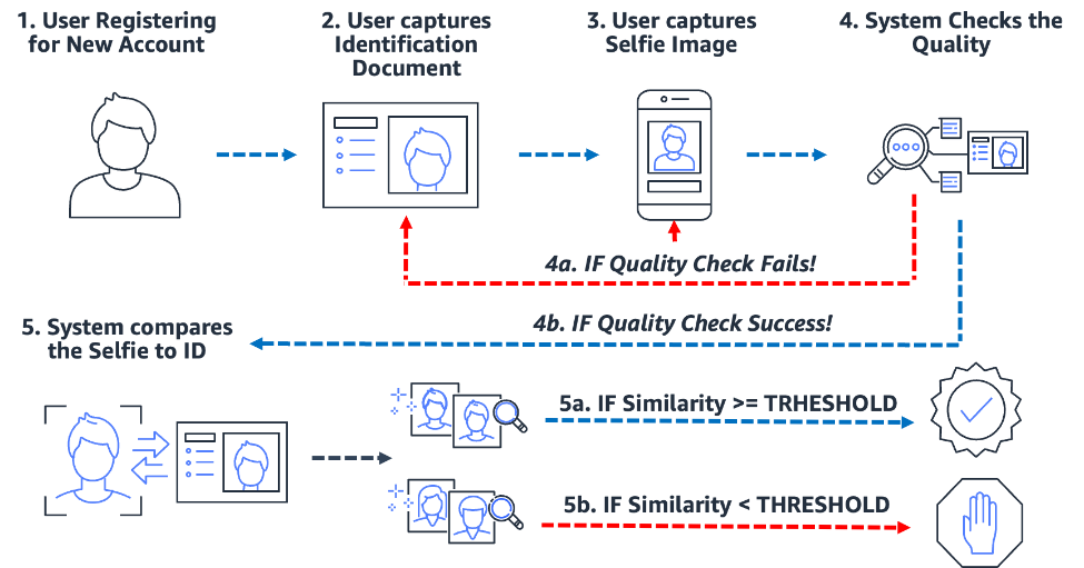
Consider the example of Julie, a new user opening a digital bank account. The solution prompts her to snap a picture of her driver’s license (step 2) and snap a selfie (step 3). After the system checks the quality of the images (step 4), it compares the face in the selfie to the face on the driver’s license (one-to-one matching) and a similarity score (step 5) is produced. If the similarity score is less than the required similarity threshold, then the onboarding attempt by Julie is rejected. This is what we call a false non-match or false rejection: the solution considered two images of the same person to be different. On the other hand, if the similarity score was greater than the required similarity, then the solution considers the two images to be the same person or a match.

Authentication: One-to-many identification

From entering a building, to checking in at a kiosk, to prompting a user for a selfie to verify their identity, this type of zero-to-low-friction authentication via facial recognition has become commonplace for many organizations. Instead of performing image-to-image matching, this authentication use case takes a single image and compares it to a searchable collection of images for a potential match. In a typical authentication use case, the user is prompted to snap a selfie, which is then compared against the faces stored in the collection. The result of the search yields zero, one, or more potential matches with corresponding similarity scores and external identifiers. If no match is returned, then the user is not authenticated; however, assuming the search returns one or more matches, the system makes the authentication decision based on the similarity scores and external identifiers. If the similarity score exceeds the required similarity threshold and the external identifier matches the expected identifier, then the user is authenticated (matched). The following diagram outlines an example face-based biometric authentication process.

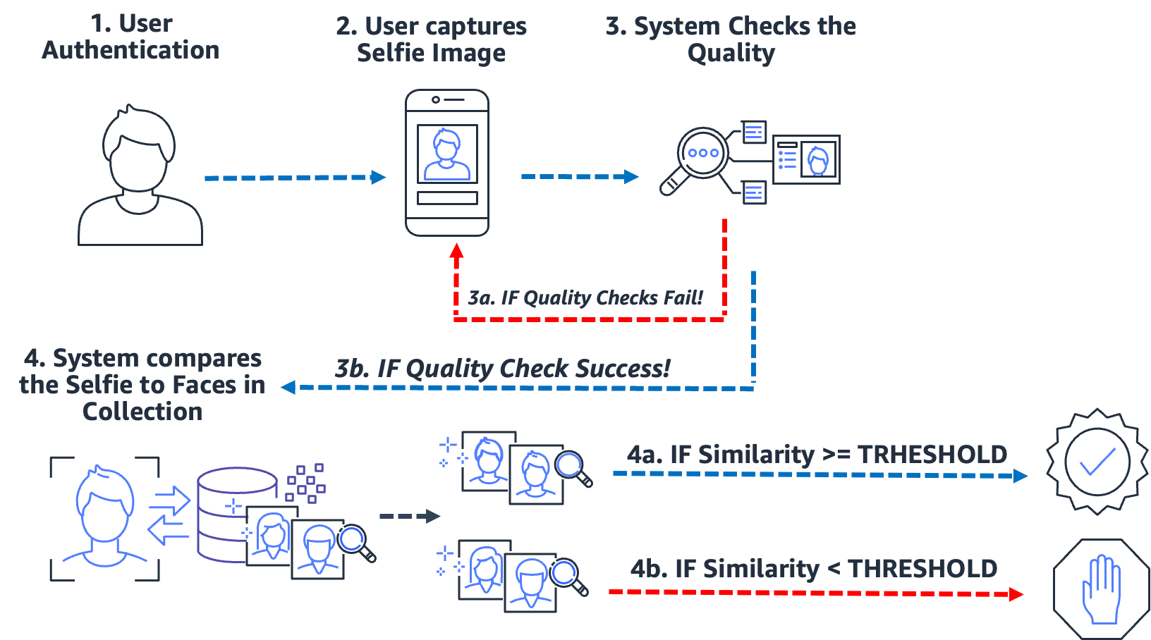
Consider the example of Jose, a gig-economy delivery driver. The delivery service authenticates delivery drivers by prompting the driver to snap a selfie before starting a delivery using the company’s mobile application. One problem gig-economy service providers face is job-sharing; essentially two or more users share the same account in order to game the system. To combat this, many delivery services use an in-car camera to snap images (step 2) of the driver at random times during a delivery (to ensure that the delivery driver is the authorized driver). In this case, Jose not only snaps a selfie at the start of his delivery, but an in-car camera snaps images of him during the delivery. The system performs quality checks (step 3) and searches (step 4) the collection of registered drivers to verify the identity of the driver. If a different driver is detected, then the gig-economy delivery service can investigate further.

A false match (false positive) occurs when the solution considered two or more images of different people to be the same person. In our use case, suppose that instead of the authorized driver, Jose he lets his brother Miguel take one of his deliveries for him. If the solution incorrectly matches Miguel’s selfie to the images of Jose, then a false match (false positive) occurs.

To combat the potential of a false matches, we recommend that collections contain several images of each subject. It’s common practice to index trusted identification documents containing a face, a selfie at time of onboarding, and selfies from the last several identification checks. Indexing several images of a subject provides the ability to aggregate the similarity scores across faces returned, thereby improving the accuracy of the identification. Additionally, external identifiers are used to limit the risk of a false acceptance. An example business rule might look something like this:

IF aggregate similarity score >= required similarity threshold AND external identifier == expected identifier THEN authenticate

Key biometric accuracy measures

In a biometric system, we’re interested in the false match rate (FMR) and false non-match rate (FNMR) based on the similarity scores from face comparisons and searches. Whether it’s an onboarding or authentication use case, biometric systems decide to accept or reject matches of a user’s face based on the similarity score of two or more images. Like any decision system, there will be errors where the system incorrectly accepts or rejects an attempt at onboarding or authentication. As part of evaluating your identity verification solution, you need to evaluate the system at various similarity thresholds to minimize false match and false non-match rates, as well as contrast those errors against the cost of making incorrect rejections and acceptances. We use FMR and FNMR as our two key metrics to evaluate facial biometric systems.

False non-match rate

When the identity verification system fails to correctly identify or authorize a genuine user, a false non-match occurs, also known as a false negative. The false non-match rate (FNMR) is a measure of how prone the system is to incorrectly identifying or authorizing a genuine user.

The FNMR is expressed as a percentage of instances where an onboarding or authentication attempt is made, where the user’s face is incorrectly rejected (a false negative) because the similarity score is below the prescribed threshold.

A true positive (TP) is when the solution considers two or more images of the same person to be the same. That is, the similarity of the comparison or search is above the required similarity threshold.

A false negative (FN) is when the solution considers two or more images of the same person to be different. That is, the similarity of the comparison or search is below the required similarity threshold.

The formula for the FNMR is:

FNMR = False Negative Count / (True Positive Count + False Negative Count)

For example, suppose we have 10,000 genuine authentication attempts but 100 are denied because their similarity to the reference image or collection falls below the specified similarity threshold. Here we have 9,900 true positives and 100 false negatives, therefore our FNMR is 1.0%

FNMR = 100 / (9900 + 100) or 1.0%

False match rate

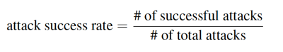
When an identity verification system incorrectly identifies or authorizes an unauthorized user as genuine, a false match occurs, also known as a false positive. The false match rate (FMR) is a measure of how prone the system is to incorrectly identifying or authorizing an unauthorized user. It’s measured by the number of false positive recognitions or authentications divided by the total number of identification attempts.

A false positive occurs when the solution considers two or more images of different people to be the same person. That is, the similarity score of the comparison or search is above the required similarity threshold. Essentially, the system incorrectly identifies or authorizes a user when it should have rejected their identification or authentication attempt.

The formula for the FMR is:

FMR = False Positive Count / (Total Attempts)

For example, suppose we have 100,000 authentication attempts but 100 bogus users are incorrectly authorized because their similarity to the reference image or collection falls above the specified similarity threshold. Here we have 100 false positives, therefore our FMR is 0.01%

FMR = 100 / (100,000) or 0.01%

False match rate vs. false non-match rate

False match rate and false non-match rate are at odds with each other. As the similarity threshold increases, the potential for a false match decreases, while the potential for a false non-match increases. Another way to think about this trade-off is that as the similarity threshold increases, the solution becomes more restrictive, making fewer low similarity matches. For example, it’s common for use cases involving public safety and security to set a match similarity threshold quite high (99 and above). Alternatively, an organization may choose a less restrictive similarity threshold (90 and above), where the impact of friction to the user is more important. The following diagram illustrates these trade-offs. The challenge for organizations is to find a threshold that minimizes both FMR and FNMR based on your organizational and application requirements.

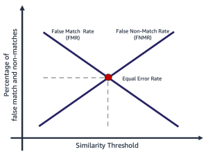
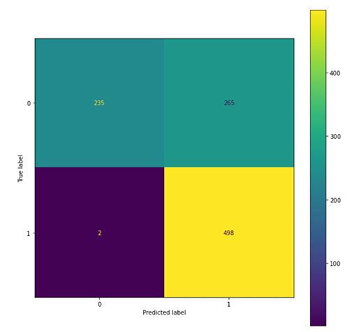
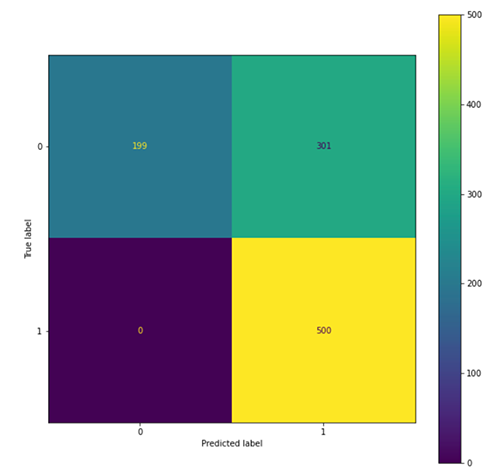
Selecting a similarity threshold depends on the business application. For example, suppose you want to limit customer friction during onboarding (a less restrictive similarity threshold, as shown in the following figure on the left). Here you might have a lower required similarity threshold, and are willing to accept the risk of onboarding users where the confidence in the match between their selfie and driver’s license is lower. By contrast, suppose you want to ensure only authorized users get into an application. Here you might operate at a quite restrictive similarity threshold (as shown in the figure on the right).

Steps for calculating false match and non-match rates

There are several of ways to calculate these two metrics. The following is a relatively simple approach of dividing the steps into gathering genuine image pairs, creating an imposter pairing (images that shouldn’t match), and finally using a probe to loop over the expected match and non-match image pairs, capturing the resulting similarity. The steps are as follows:

1. Gather a genuine sample image set. We recommend starting with a set of image pairs and assigning an external identifier, which is used to make an official match determination. The pair consists of the following images:
   1. Source image – Your trusted source image, for example a driver’s license.
   2. Target image – Your selfie or image you are going to compare with.
2. Gather an image set of imposter matches. These are pairs of images where the source and target don’t match. This is used to assess the FMR (the probability that the system will incorrectly match the faces of two different users). You can create an imposter image set using the image pairs by creating a Cartesian product of the images then filtering and sampling the result.
3. Probe the genuine and imposter match sets by looping over the image pairs, comparing the source and imposter target and capturing the resulting similarity.
4. Calculate FMR and FNMR by calculating the false positives and false negatives at different minimum similarity thresholds.

You can assess the cost of FMR and FNMR at different similarity thresholds relative to your application’s need.

Step 1: Gather genuine image pair samples

Choosing a representative sample of image pairs to evaluate is critical when evaluating an identity verification service. The first step is to identify a genuine set of image pairs. These are known source and target images of a user. The genuine image pairing is used to assess the FNMR, essentially the probability that the system won’t match two faces of the same person. One of the first questions often asked is “How many image pairs are necessary?” The answer is that it depends on your use case, but the general guidance is the following:

• Between 100–1,000 image pairs provides a measure of feasibility
• Up to 10,000 images pairs is large enough to measure variability between images
• More than 10,000 image pairs provides a measure of operational quality and generalizability

More data is always better; however, as a starting point, use at least 1,000 image pairs. However, it’s not uncommon to use more than 10,000 image pairs to zero in on an acceptable FNMR or FMR for a given business problem.

The following is a sample image pair mapping file. We use the image pair mapping file to drive the rest of the evaluation process.

Step 2: Generate an imposter image pair set

Now that you have a file of genuine image pairs, you can create a Cartesian product of target and source images where the external identifiers don’t mach. This produces source-to-target pairs that shouldn’t match. This pairing is used to assess the FMR, essentially the probability the system will match the face of one user to a face of a different user.

Step 3: Probe the genuine and imposter image pair sets

Using a driver program, we apply the Amazon Rekognition CompareFaces API over the image pairs and capture the similarity. You can also capture additional information like pose, quality, and other results of the comparison. The similarity scores are used to calculate the false match and non-match rates in the following step.

In the following code snippet, we apply the CompareFaces API to all the image pairs and populate all the similarity scores in a table:

obj = s3.get_object(Bucket= bucket_name , Key = csv_file)

df = pd.read_csv(io.BytesIO(obj['Body'].read()), encoding='utf8')
def compare_faces(source_file, target_file, threshold = 0):
    response=rekognition.compare_faces(SimilarityThreshold=threshold,
                                        SourceImage={'S3Object': {
                                                    'Bucket': bucket_name,
                                                    'Name':source_file}},
                                        TargetImage={'S3Object': {
                                                    'Bucket': bucket_name,
                                                    'Name':target_file}})
df_similarity = df.copy()
df_similarity["SIMILARITY"] = None
for index, row in df.iterrows():
    source_file = dataset_folder + row["SOURCE"]
    target_file = dataset_folder + row["TARGET"]
    response_score = compare_faces(source_file, target_file)
    df_similarity._set_value(index,"SIMILARITY", response_score)
    df_similarity.head()

The code snippet gives the following output.

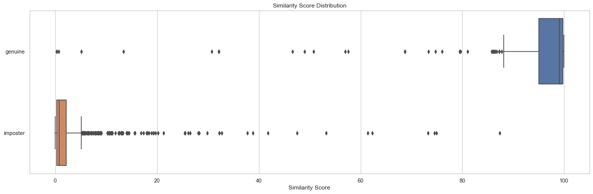
Distribution analysis of similarity scores by tests are a starting point to understand the similarity score by image pairs. The following code snippet and output chart shows a simple example of the distribution of similarity score by test set as well as resulting descriptive statistics:

sns.boxplot(data=df_similarity,
            x=df_similarity["SIMILARITY"],
            y=df_similarity["TEST"]).set(xlabel='Similarity Score',
            ylabel=None,
            title = "Similarity Score Distribution")
plt.show()

df_descriptive_stats = pd.DataFrame(columns=['test','count', 'min' , 'max', 'mean', 'median', 'std'])

tests = ["Genuine", "Imposter"]

for test in tests:
    count = df_similarity['SIMILARITY'].loc[df_similarity['TEST'] == test].count()
    mean = df_similarity['SIMILARITY'].loc[df_similarity['TEST'] == test].mean()
    max_ = df_similarity['SIMILARITY'].loc[df_similarity['TEST'] == test].max()
    min_ = df_similarity['SIMILARITY'].loc[df_similarity['TEST'] == test].min()
    median = df_similarity['SIMILARITY'].loc[df_similarity['TEST'] == test].median()
    std = df_similarity['SIMILARITY'].loc[df_similarity['TEST'] == test].std()

    new_row = {'test': test,
                'count': count,
                'min': min_,
                'max': max_,
                'mean': mean,
                'median':median,
                'std': std}
    df_descriptive_stats = df_descriptive_stats.append(new_row,
    ignore_index=True)

df_descriptive_stats

In this example, we can see that the mean and median similarity for genuine face pairs was 91.7 and 99.1, whereas for the imposter pairs was 2.8 and 0.8, respectively. As expected, this shows the high similarity scores for genuine image pairs and low similarity scores for imposter image pairs.

Step 4: Calculate FMR and FNMR at different similarity threshold levels

In this step, we calculate the false match and non-match rates at different thresholds of similarity. To do this, we simply loop through similarity thresholds (for example, 90–100). At each selected similarity threshold, we calculate our confusion matrix containing true positive, true negative, false positive, and false negative counts, which are used to calculate the FMR and FNMR at each selected similarity.

To do this, we create a function that returns the false positive and negative counts, and loop through a range of similarity scores (90–100):

similarity_thresholds = [80,85,90,95,96,97,98,99]

# create output df
df_cols = ['Similarity Threshold', 'TN' , 'FN', 'TP', 'FP', 'FNMR (%)', 'FMR (%)']
comparison_df = pd.DataFrame(columns=df_cols)

# create columns for y_actual and y_pred
df_analysis = df_similarity.copy()
df_analysis["y_actual"] = None
df_analysis["y_pred"] = None

for threshold in similarity_thresholds:
    # Create y_pred and y_actual columns, 1 == match, 0 == no match
    for index, row in df_similarity.iterrows():
        # set y_pred
        if row["SIMILARITY"] >= threshold:
            df_analysis._set_value(index,"y_pred", 1)
        else:
            df_analysis._set_value(index,"y_pred", 0)

        # set y_actual
        if row["TEST"] == "Genuine":
            df_analysis._set_value(index,"y_actual", 1)
        else:
            df_analysis._set_value(index,"y_actual", 0)

    tn, fp, fn, tp = confusion_matrix(df_analysis['y_actual'].tolist(),
                                      df_analysis['y_pred'].tolist()).ravel()
    FNMR = fn / (tp + fn)
    FMR = fp / (tn+fp+fn+tp)

    new_row = {'Similarity Threshold': threshold,
                'TN': tn,
                'FN': fn,
                'TP': tp,
                'FP': fp,
                'FNMR (%)':FNMR,
                'FMR (%)': FMR}
    comparison_df = comparison_df.append(new_row,ignore_index=True)

comparison_df

The following table shows the results of the counts at each similarity threshold.

How does the similarity threshold impact false non-match rate?

Suppose we have 1,000 genuine user onboarding attempts, and we reject 10 of these attempts based on a required minimum similarity of 95% to be considered a match. Here we reject 10 genuine onboarding attempts (false negatives) because their similarity falls below the specified minimum required similarity threshold. In this case, our FNMR is 1.0%.

FNMR = False Negative Count / (True Positive Count + False Negative Count)

FNMR = 10 / (990 + 10) or 1.0%

By contrast, suppose instead of having 1,000 genuine users to onboard, we have 990 genuine users and 10 imposter users (false positive). At a 95% minimum similarity, suppose we accept all 1,000 users as genuine. Here we would have a 1% FMR.

FMR = False Positive Count / (Total Attempts)

FMR = 10 / (1,000) or 1.0%

Assessing costs of FMR and FNMR at onboarding

In an onboarding use case, the cost of a false non-match (a rejection) is generally associated with additional user friction or loss of a registration. For example, in our banking use case, suppose Julie presents two images of herself but is incorrectly rejected at time of onboarding because the similarity between the two images falls below the selected similarity (a false non-match). The financial institution may risk losing Julie as a potential customer, or it may cause Julie additional friction by requiring her to perform steps to prove her identity.

Conversely, suppose the two images of Julie are of different people and Julie’s onboarding should have been rejected. In the case where Julie is incorrectly accepted (a false match), the cost and risk to the financial institution is quite different. There could be regulatory issues, risk of fraud, and other risks associated with financial transactions.

Responsible use

Artificial intelligence (AI) applied through machine learning (ML) will be one of the most transformational technologies of our generation, tackling some of humanity’s most challenging problems, augmenting human performance, and maximizing productivity. Responsible use of these technologies is key to fostering continued innovation. AWS is committed to developing fair and accurate AI and ML services and providing you with the tools and guidance needed to build AI and ML applications responsibly.

As you adopt and increase your use of AI and ML, AWS offers several resources based on our experience to assist you in the responsible development and use of AI and ML:

• Use cases that involve public safety
• AWS Service Terms
• Resources and tools provided by AWS on responsible use of AI and ML

Best practices and common mistakes to avoid

In this section, we discuss the following best practices:

• Use a large enough sample of images
• Avoid open-source and synthetic face datasets
• Avoid manual and synthetic image manipulation
• Check image quality at time of evaluation and over time
• Monitor FMR and FNMR over time
• Use a human in the loop review
• Stay up to date with Amazon Rekognition

Use a large enough sample of images

Use a large enough but reasonable sample of images. What is a reasonable sample size? It depends on the business problem. If you’re an employer and have 10,000 employees that you want to authenticate, then using all 10,000 images is probably reasonable. However, suppose you’re an organization with millions of customers that you want to onboard. In this case, taking a representative sample of customers such as 5,000–20,000 is probably sufficient. Here is some guidance on the sample size:

• A sample size of 100 – 1,000 image pairs proves feasibility
• A sample size of 1,000 – 10,000 image pairs is useful to measure variability between images
• A sample size of 10,000 – 1 million image pairs provides a measure of operational quality and generalizability

The key with sampling image pairs is to ensure that the sample provides enough variability across the population of faces in your application. You can further extend your sampling and testing to include demographic information like skin tone, gender, and age.

Avoid open-source and synthetic face datasets

There are dozens of curated open-source facial image datasets as well as astonishingly realistic synthetic face sets that are often used in research and to study feasibility. The challenge is that these datasets are generally not useful for 99% of real-world use cases simply because they aren’t representative of the cameras, faces, and quality of the images your application is likely to encounter in the wild. Although they’re useful for application development, the accuracy measures of these image sets don’t generalize to what you’ll encounter in your own application. Instead, we recommend starting with a representative sample of real images from your solution, even if the sample image pairs are small (under 1,000).

Avoid manual and synthetic image manipulation

There are often edge cases that people are interested in understanding. Things like image capture quality or obfuscations of specific facial features are always of interest. For example, we often get asked about the impact of age and image quality on facial recognition. You could simply synthetically age a face or manipulate the image to make the subject appear older, or manipulate the image quality, but this doesn’t translate well to real-world aging of images. Instead, our recommendation is to gather a representative sample of real-world edge cases you’re interested in testing.

Check image quality at time of evaluation and over time

Camera and application technology changes quite rapidly over time. As a best practice, we recommend monitoring image quality over time. From the size of faces captured (using bounding boxes), to the brightness and sharpness of an image, to the pose of a face, as well as potential obfuscations (hats, sunglasses, beards, and so on), all of these image and facial features change over time.

Monitor FNMR and FMR over time

Changes occur, whether it’s the images, the application, or the similarity thresholds used in the application. It’s important to periodically monitor false match and non-match rates over time. Changes in the rates (even subtle changes) can often point to upstream challenges with the application or how the application is being used. Changes to similarity thresholds and business rules used to make accept or reject decisions can have major impact on onboarding and authentication user experiences.

Use a human in the loop review

Identity verification systems make automated decisions to match and non-match based on similarity thresholds and business rules. Besides regulatory and internal compliance requirements, an important process in any automated decision system is to utilize human reviewers as part of the ongoing monitoring of the decision process. Human oversight of these automated decisioning systems provides validation and continuous improvement as well as transparency into the automated decision-making process.

Stay up to date with Amazon Rekognition

The Amazon Recognition faces model is updated periodically (usually annually), and is currently on version 6. This updated version made important improvements to accuracy and indexing. It’s important to stay up to date with new model versions and understand how to use these new versions in your identity verification application. When new versions of the Amazon Rekognition face model are launched, it’s good practice to rerun your identity verification evaluation process and determine any potential impacts (positive and negative) to your false match and non-match rates.

Conclusion

This post discusses the key elements needed to evaluate the performance aspect of your identity verification solution in terms of various accuracy metrics. However, accuracy is only one of the many dimensions that you need to evaluate when choosing a particular content moderation service. It’s critical that you include other parameters, such as the service’s total feature set, ease of use, existing integrations, privacy and security, customization options, scalability implications, customer service, and pricing.

To learn more about identity verification in Amazon Rekognition, visit Identity Verification using Amazon Rekognition.

About the Authors

Mike Ames is a data scientist turned identity verification solution specialist, with extensive experience developing machine learning and AI solutions to protect organizations from fraud, waste, and abuse. In his spare time, you can find him hiking, mountain biking, or playing freebee with his dog Max.

Amit Gupta is a Senior AI Services Solutions Architect at AWS. He is passionate about enabling customers with well-architected machine learning solutions at scale.

Zuhayr Raghib is an AI Services Solutions Architect at AWS. Specializing in applied AI/ML, he is passionate about enabling customers to use the cloud to innovate faster and transform their businesses.

Marcel Pividal is a Sr. AI Services Solutions Architect in the World-Wide Specialist Organization. Marcel has more than 20 years of experience solving business problems through technology for fintechs, payment providers, pharma, and government agencies. His current areas of focus are risk management, fraud prevention, and identity verification.

Read More