With quantum computers poised to take a big step forward, we speak to an Amazon Scholar who has spent two decades driving the technology to realize its enormous potential.Read More
Amazon SCOT announces 2022 INFORMS Scholars
Program was established to help expand the pipeline of operations research, management science, and analytics talent from underrepresented backgrounds.Read More
reMARS revisited: Autonomous mobile robots and safety design
Examining the opportunities for creating a functional safety certification for autonomous mobile robots.Read More
Improve price performance of your model training using Amazon SageMaker heterogeneous clusters
This post is co-written with Chaim Rand from Mobileye.
Certain machine learning (ML) workloads, such as training computer vision models or reinforcement learning, often involve combining the GPU- or accelerator-intensive task of neural network model training with the CPU-intensive task of data preprocessing, like image augmentation. When both types of tasks run on the same instance type, the data preprocessing gets bottlenecked on CPU, leading to lower GPU utilization. This issue becomes worse with time as the throughput of newer generations of GPUs grows at a steeper pace than that of CPUs.
To address this issue, in July 2022, we launched heterogeneous clusters for Amazon SageMaker model training, which enables you to launch training jobs that use different instance types in a single job. This allows offloading parts of the data preprocessing pipeline to compute-optimized instance types, whereas the deep neural network (DNN) task continues to run on GPU or accelerated computing instance types. Our benchmarks show up to 46% price performance benefit after enabling heterogeneous clusters in a CPU-bound TensorFlow computer vision model training.
For a similar use case, Mobileye, an autonomous vehicle technologies development company, had this to share:
“By moving CPU-bound deep learning computer vision model training to run over multiple instance types (CPU and GPU/ML accelerators), using a tf.data.service based solution we’ve built, we managed to reduce time to train by 40% while reducing the cost to train by 30%. We’re excited about heterogeneous clusters allowing us to run this solution on Amazon SageMaker.”
— AI Engineering, Mobileye
In this post, we discuss the following topics:
- How heterogeneous clusters help remove CPU bottlenecks
- When to use heterogeneous clusters, and other alternatives
- Reference implementations in PyTorch and TensorFlow
- Performance benchmark results
- Heterogeneous clusters at Mobileye
AWS’s accelerated computing instance family includes accelerators from AWS custom chips (AWS Inferentia, AWS Trainium), NVIDIA (GPUs), and Gaudi accelerators from Habana Labs (an Intel company). Note that in this post, we use the terms GPU and accelerator interchangeably.
How heterogeneous clusters remove data processing bottlenecks
Data scientists who train deep learning models aim to maximize training cost-efficiency and minimize training time. To achieve this, one basic optimization goal is to have high GPU utilization, the most expensive and scarce resource within the Amazon Elastic Compute Cloud (Amazon EC2) instance. This can be more challenging with ML workloads that combine the classic GPU-intensive neural network model’s forward and backward propagation with CPU-intensive tasks, such as data processing and augmentation in computer vision or running an environment simulation in reinforcement learning. These workloads can end up being CPU bound, where having more CPU would result in higher throughput and faster and cheaper training as existing accelerators are partially idle. In some cases, CPU bottlenecks can be solved by switching to another instance type with a higher CPU:GPU ratio. However, there are situations where switching to another instance type may not be possible due to the instance family’s architecture, storage, or networking dependencies.
In such situations, you have to increase the amount of CPU power by mixing instance types: instances with GPUs together with CPU. Summed together, this results in an overall higher CPU:GPU ratio. Until recently, SageMaker training jobs were limited to having instances of a single chosen instance type. With SageMaker heterogeneous clusters, data scientists can easily run a training job with multiple instance types, which enables offloading some of the existing CPU tasks from the GPU instances to dedicated compute-optimized CPU instances, resulting in higher GPU utilization and faster and more cost-efficient training. Moreover, with the extra CPU power, you can have preprocessing tasks that were traditionally done offline as a preliminary step to training become part of your training job. This makes it faster to iterate and experiment over both data preprocessing and DNN training assumptions and hyperparameters.
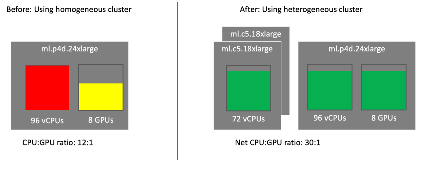
For example, consider a powerful GPU instance type, ml.p4d.24xlarge (96 vCPU, 8 x NVIDIA A100 GPUs), with a CPU:GPU ratio of 12:1. Let’s assume your training job needs 20 vCPUs to preprocess enough data to keep one GPU 100% utilized. Therefore, to keep all 8 GPUs 100% utilized, you need a 160 vCPUs instance type. However, ml.p4d.24xlarge is short of 64 vCPUs, or 40%, limiting GPU utilization to 60%, as depicted on the left of the following diagram. Would adding another ml.p4d.24xlarge instance help? No, because the job’s CPU:GPU ratio would remain the same.
With heterogeneous clusters, we can add two ml.c5.18xlarge (72 vCPU), as shown on the right of the diagram. The net total vCPU in this cluster is 210 (96+2*72), leading to a CPU:GPU ratio to 30:1. Each of these compute-optimized instances will be offloaded with a data preprocessing CPU-intensive task, and will allow efficient GPU utilization. Despite the extra cost of the ml.c5.18xlarge, the higher GPU utilization allows faster processing, and therefore higher price performance benefits.
When to use heterogeneous clusters, and other alternatives
In this section, we explain how to identify a CPU bottleneck, and discuss solving it using instance type scale up vs. heterogeneous clusters.
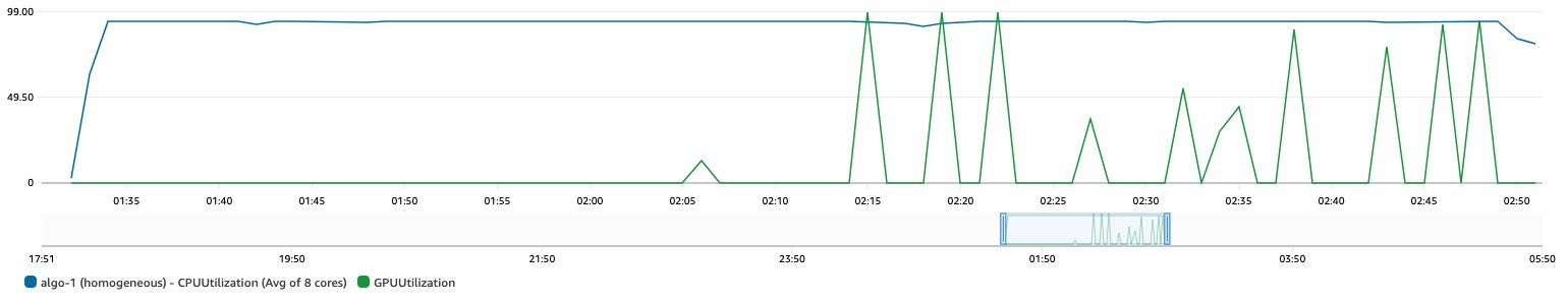
The quick way to identify a CPU bottleneck is to monitor CPU and GPU utilization metrics for SageMaker training jobs in Amazon CloudWatch. You can access these views from the AWS Management Console within the training job page’s instance metrics hyperlink. Pick the relevant metrics and switch from 5-minute to 1-minute resolution. Note that the scale is 100% per vCPU or GPU, so the utilization rate for an instance with 4 vCPUs/GPUs could be as high as 400%. The following figure is one such example from CloudWatch metrics, where CPU is approximately 100% utilized, indicating a CPU bottleneck, whereas GPU is underutilized.
For detailed diagnosis, run the training jobs with Amazon SageMaker Debugger to profile resource utilization status, statistics, and framework operations, by adding a profiler configuration when you construct a SageMaker estimator using the SageMaker Python SDK. After you submit the training job, review the resulting profiler report for CPU bottlenecks.
If you conclude that your job could benefit from a higher CPU:GPU compute ratio, first consider scaling up to another instance type in the same instance family, if one is available. For example, if you’re training your model on ml.g5.8xlarge (32 vCPUs, 1 GPU), consider scaling up to ml.g5.16xlarge (64 vCPUs, 1 GPU). Or, if you’re training your model using multi-GPU instance ml.g5.12xlarge (48 vCPUs, 4 GPUs), consider scaling up to ml.g5.24xlarge (96 vCPUs, 4 GPUs). Refer to the G5 instance family specification for more details.
Sometimes, scaling up isn’t an option, because there is no instance type with a higher vCPU:GPU ratio in the same instance family. For example, if you’re training the model on ml.trn1.32xlarge, ml.p4d.24xlarge, or ml.g5.48xlarge, you should consider heterogeneous clusters for SageMaker model training.
Besides scaling up, we’d like to note that there are additional alternatives to a heterogeneous cluster, like NVIDIA DALI, which offloads image preprocessing to the GPU. For more information, refer to Overcoming Data Preprocessing Bottlenecks with TensorFlow Data Service, NVIDIA DALI, and Other Methods.
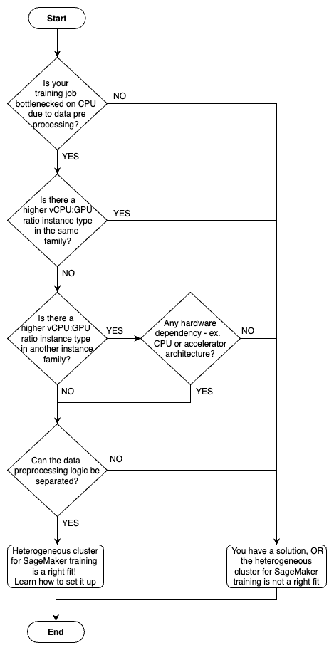
To simplify decision-making, refer to the following flowchart.
How to use SageMaker heterogeneous clusters
To get started quickly, you can directly jump to the TensorFlow or PyTorch examples provided as part of this post.
In this section, we walk you through how to use a SageMaker heterogeneous cluster with a simple example. We assume that you already know how to train a model with the SageMaker Python SDK and the Estimator class. If not, refer to Using the SageMaker Python SDK before continuing.
Prior to this feature, you initialized the training job’s Estimator class with the InstanceCount and InstanceType parameters, which implicitly assumes you only have a single instance type (a homogeneous cluster). With the release of heterogeneous clusters, we introduced the new sagemaker.instance_group.InstanceGroup class. This represents a group of one or more instances of a specific instance type, designed to carry a logical role (like data processing or neural network optimization. You can have two or more groups, and specify a custom name for each instance group, the instance type, and the number of instances for each instance group. For more information, refer to Using the SageMaker Python SDK and Using the Low-Level SageMaker APIs.
After you have defined the instance groups, you need to modify your training script to read the SageMaker training environment information that includes heterogeneous cluster configuration. The configuration contains information such as the current instance groups, the current hosts in each group, and in which group the current host resides with their ranking. You can build logic in your training script to assign the instance groups to certain training and data processing tasks. In addition, your training script needs to take care of inter-instance group communication or distributed data loading mechanisms (for example, tf.data.service in TensorFlow or generic gRPC client-server) or any other framework (for example, Apache Spark).
Let’s go through a simple example of launching a heterogeneous training job and reading the environment configuration at runtime.
- When defining and launching the training job, we configure two instance groups used as arguments to the SageMaker estimator:
from sagemaker.instance_group import InstanceGroup data_group = InstanceGroup("data_group", "ml.c5.18xlarge", 2) dnn_group = InstanceGroup("dnn_group", "ml.p4d.24xlarge", 1) from sagemaker.pytorch import PyTorch estimator = PyTorch(..., entry_point='launcher.py', instance_groups=[data_group, dnn_group] ) - On the entry point training script (named
launcher.py), we read the heterogeneous cluster configuration to whether the instance will run the preprocessing or DNN code:
With this, let’s summarize the tasks SageMaker does on your behalf, and the tasks that you are responsible for.
SageMaker performs the following tasks:
- Provision different instance types according to instance group definition.
- Provision input channels on all or specific instance groups.
- Distribute training scripts and dependencies to instances.
- Set up an MPI cluster on a specific instance group, if defined.
You are responsible for the following tasks:
- Modify your start training job script to specify instance groups.
- Implement a distributed data pipeline (for example,
tf.data.service). - Modify your entry point script (see
launcher.pyin the example notebook) to be a single entry point that will run on all the instances, detect which instance group it’s running in, and trigger the relevant behavior (such as data processing or DNN optimization). - When the training loop is over, you must make sure that your entry point process exits on all instances across all instance groups. This is important because SageMaker waits for all the instances to finish processing before it marks the job as complete and stops billing. The
launcher.pyscript in the TensorFlow and PyTorch example notebooks provides a reference implementation of signaling data group instances to exit when DNN group instances finish their work.
Example notebooks for SageMaker heterogeneous clusters
In this section, we provide a summary of the example notebooks for both TensorFlow and PyTorch ML frameworks. In the notebooks, you can find the implementation details, walkthroughs on how the code works, code snippets that you could reuse in your training scripts, flow diagrams, and cost-comparison analysis.
Note that in both examples, you shouldn’t expect the model to converge in a meaningful way. Our intent is only to measure the data pipeline and neural network optimization throughput expressed in epoch/step time. You must benchmark with your own model and dataset to produce price performance benefits that match your workload.
Heterogeneous cluster using a tf.data.service based distributed data loader (TensorFlow)
This notebook demonstrates how to implement a heterogeneous cluster for SageMaker training using TensorFlow’s tf.data.service based distributed data pipeline. We train a deep learning computer vision model Resnet50 that requires CPU-intensive data augmentation. It uses Horvod for multi-GPU distributed data parallelism.
We run the workload in two configurations: first as a homogeneous cluster, single ml.p4d.24xlarge instance, using a standard tf.data pipeline that showcases CPU bottlenecks leading to lower GPU utilization. In the second run, we switch from a single instance type to two instance groups using a SageMaker heterogeneous cluster. This run offloads some of the data processing to additional CPU instances (using tf.data.service).
We then compare the homogeneous and heterogeneous configurations and find key price performance benefits. As shown in the following table, the heterogeneous job (86ms/step) is 2.2 times faster to train than the homogeneous job (192ms/step), making it 46% cheaper to train a model.
| Example 1 (TF) | ml.p4d.24xl | ml.c5.18xl | Price per Hour* | Average Step Time | Cost per Step | Price Performance Improvement |
| Homogeneous | 1 | 0 | $37.688 | 192 ms | $0.201 | . |
| Heterogeneous | 1 | 2 | $45.032 | 86 ms | $0.108 | 46% |
* Price per hour is based on us-east-1 SageMaker on-demand pricing
This speedup is made possible by utilizing the extra vCPU, provided by the data group, and faster preprocessing. See the notebook for more details and graphs.
Heterogeneous cluster using a gRPC client-server based distributed data loader (PyTorch)
This notebook demonstrates a sample workload using a heterogeneous cluster for SageMaker training using a gRPC client-server based distributed data loader. This example uses a single GPU. We use the PyTorch model based on the following official MNIST example. The training code has been modified to be heavy on data preprocessing. We train this model in both homogeneous and heterogeneous cluster modes, and compare price performance.
In this example, we assumed the workload can’t benefit from multiple GPUs, and has dependency on a specific GPU architecture (NVIDIA V100). We ran both homogeneous and heterogeneous training jobs, and found key price performance benefits, as shown in the following table. The heterogeneous job (1.19s/step) is 6.5 times faster to train than the homogeneous job (0.18s/step), making it 77% cheaper to train a model.
| Example 2 (PT) | ml.p3.2xl | ml.c5.9xl | Price per Hour* | Average Step Time | Cost per Step | Price Performance Improvement |
| Homogeneous | 1 | 0 | $3.825 | 1193 ms | $0.127 | . |
| Heterogeneous | 1 | 1 | $5.661 | 184 ms | $0.029 | 77% |
* Price per hour is based on us-east-1 SageMaker on-demand pricing
This is possible because with a higher CPU count, we could use 32 data loader workers (compared to 8 with ml.p3.2xlarge) to preprocess the data and kept GPU close to 100% utilized at frequent intervals. See the notebook for more details and graphs.
Heterogeneous clusters at Mobileye
Mobileye, an Intel company, develops Advanced Driver Assistance Systems (ADAS) and autonomous vehicle technologies with the goal of revolutionizing the transportation industry, making roads safer, and saving lives. These technologies are enabled using sophisticated computer vision (CV) models that are trained using SageMaker on large amounts of data stored in Amazon Simple Storage Service (Amazon S3). These models use state-of-the-art deep learning neural network techniques.
We noticed that for one of our CV models, the CPU bottleneck was primarily caused by heavy data preprocessing leading to underutilized GPUs. For this specific workload, we started looking at alternative solutions, evaluated distributed data pipeline technologies with heterogeneous clusters based on EC2 instances, and came up with reference implementations for both TensorFlow and PyTorch. The release of the SageMaker heterogeneous cluster allows us to run this and similar workloads on SageMaker to achieve improved price performance benefits.
Considerations
With the launch of the heterogeneous cluster feature, SageMaker offers a lot more flexibility in mixing and matching instance types within your training job. However, consider the following when using this feature:
- The heterogeneous cluster feature is available through SageMaker PyTorch and TensorFlow framework estimator classes. Supported frameworks are PyTorch v1.10 or later and TensorFlow v2.6 or later.
- All instance groups share the same Docker image.
- All instance groups share the same training script. Therefore, your training script should be modified to detect which instance group it belongs to and fork runs accordingly.
- The training instances hostnames (for example, alog-1, algo-2, and so on) are randomly assigned, and don’t indicate which instance group they belong to. To get the instance’s role, we recommend getting its instance group membership during runtime. This is also relevant when reviewing logs in CloudWatch, because the log stream name
[training-job-name]/algo-[instance-number-in-cluster]-[epoch_timestamp]has the hostname. - A distributed training strategy (usually an MPI cluster) can be applied only to one instance group.
- SageMaker Managed Warm Pools and SageMaker Local Mode cannot currently be used with heterogeneous cluster training.
Conclusion
In this post, we discussed when and how to use the heterogeneous cluster feature of SageMaker training. We demonstrated a 46% price performance improvement on a real-world use case and helped you get started quickly with distributed data loader (tf.data.service and gRPC client-server) implementations. You can use these implementations with minimal code changes in your existing training scripts.
To get started, try out our example notebooks. To learn more about this feature, refer to Train Using a Heterogeneous Cluster.
About the authors
 Gili Nachum is a senior AI/ML Specialist Solutions Architect who works as part of the EMEA Amazon Machine Learning team. Gili is passionate about the challenges of training deep learning models, and how machine learning is changing the world as we know it. In his spare time, Gili enjoy playing table tennis.
 Hrushikesh Gangur is a principal solutions architect for AI/ML startups with expertise in both ML Training and AWS Networking. He helps startups in Autonomous Vehicle, Robotics, CV, NLP, MLOps, ML Platform, and Robotics Process Automation technologies to run their business efficiently and effectively on AWS. Prior to joining AWS, Hrushikesh acquired 20+ years of industry experience primarily around Cloud and Data platforms.
 Gal Oshri is a Senior Product Manager on the Amazon SageMaker team. He has 7 years of experience working on Machine Learning tools, frameworks, and services.
 Chaim Rand is a machine learning algorithm developer working on deep learning and computer vision technologies for Autonomous Vehicle solutions at Mobileye, an Intel Company. Check out his blogs.
Reduce food waste to improve sustainability and financial results in retail with Amazon Forecast
With environmental, social, and governance (ESG) initiatives becoming more important for companies, our customer, one of Greater China region’s top convenience store chains, has been seeking a solution to reduce food waste (currently over $3.5 million USD per year). Doing so will allow them to not only realize substantial operating savings, but also support corporate sustainability goals.
In this post, we focus on forecasting demand of freshly prepared food by retail convenience stores. Our customer sells ready-to-eat food items with a short shelf life—typically 2–3 days. They faced two challenges: how to reduce food waste, and how to manage forecast models for over 10,000 SKUs and thousands of stores efficiently and at scale.
With Amazon Forecast, and support from the AWS ProServe team and AWS Machine Learning Solutions Lab, our customer—with limited internal data scientists—now has state-of-the-art forecasting capabilities. Within a few months, this forecasting solution has helped them reduce product waste by 37%, resulting in cost savings of 22% across 168 stores and three merchandise categories.
To achieve these operational benefits, they implemented a number of best practice processes, including a fast data iteration and testing cycle, and parallel testing to find optimal data combinations. They also established data processing and forecasting pipelines, which can scale to thousands of stores and product categories, and developed a scalable reference architecture to be used for future extensions.
The fresh foods ESG challenge
In addition to selling environmentally sustainable products, it’s also important for the retail industry to strive for environmentally friendly processes that minimize waste. Advanced inventory forecasting using machine learning (ML) allows retail stores to maximize sales and minimize waste through more effective inventory management and turnover. Inventory that can’t be sold is a problem for convenience store chains—it drives financial losses and furthers negative environmental effects through excess usage of energy inputs and inefficient production processes. And due to large volumes, short-dated fresh food items can play a big role in both financial and sustainability results.
Besides having a short shelf life, additional demand forecasting challenges for fresh food include rapid turnover, frequent new product launches, and high SKU volumes. Specifically:
- Compared to other categories, short-dated perishables must be sold within a short time window, otherwise they will expire and be discarded. Therefore, accurate forecasting is more important than for items that can be stored and sold over a longer time period.
- New product launches are frequent, making forecasting more challenging at the SKU-level (the cold start problem).
- A large number of items can cause model management issues for traditional algorithms such as ARIMA, which are configured for each item. Many models will need to be maintained, which is both costly and hard to scale.
Inventory forecasting
Amazon Forecast is a fully managed AI/ML service from AWS, and includes both statistical and deep learning algorithms that are based on over 20 years of forecasting experience. With item-level ensemble modeling and automatic model hyperparameter optimization, it provides forecasts that are up to 40% more accurate that using traditional methods alone. In addition, features such as predictor retraining can reduce training time and cost by up to 50%.
To optimize inventory forecasting, we looked at the main drivers of demand. Even within the fresh food category, there are items that are more popular—with higher inventory turnover—and items that sell slower. By separating popular from unpopular items and training predictors, we found that predictors can fit the dataset better and enhance model accuracy with different statistical distributions. In addition, because Forecast provides probabilistic forecasts based on customer-selected quantiles, we set up prediction quantiles based on item expiration dates and item profitability.
To implement demand forecasting that enhances sustainability, we also considered industry-specific properties:
- Short lead times
- High order frequencies
- Product alternatives and substitutes
- Consumer psychology (often, consumers are more likely to make a purchase if they have a diverse set of products to select from)
To balance shelf diversity against inventory wastage, we not only produced daily demand forecasts, but also performed what-if analyses to optimize promotion of unsold items before they expire.
We were able to incorporate these considerations and address our customer’s requirements with Forecast. In the next section, we walk through how the customer solution has been created in more detail.
Solution overview
To train a predictor, training data is ingested into data storage from a data source, using one of the formats supported by Forecast. Amazon Simple Storage Service (Amazon S3) is an object storage service offering industry-leading scalability, data availability, security, and performance. In the ingestion phase, we transform data from our source to the Forecast dataset format. Forecast uses three types of data: target time series (TTS), which is required, and related time series (RTS) and item metadata (IM), both of which are optional.
We started with the most-wasted SKUs at the stores that had the most waste. To forecast each store’s daily demand, we first started with time series (revenues, inventories, promotions) and then fine-tuned our approach based on store properties such as whether it’s a franchise or company-owned store, store type, restroom availability, store size (small or large), and store age. We also used industry knowledge, such as local holidays, promotions, weather, and daily traffic. Our TTS dataset consisted of timestamp, item ID, and demand; RTS consisted of timestamp, item ID, discount, inventory, and weather; and the IM dataset consisted of item ID, category, and store infrastructures. To quantify the importance of these features on our forecasts, we used explainability—a Forecast built-in feature that measures the relative impact of different attributes on forecast values.
A dataset must be created and associated with a dataset group to train the predictor. When creating a predictor, Forecast automatically selects the right algorithms, tunes hyperparameters, and performs ensemble modeling. In an interesting finding from this case, we used cross-COVID-19 data (from 2018–2021) to train the model and found that we didn’t need to add other COVID-19 features such as number of daily confirmed cases. The deep neural network models can learn directly from daily revenue.
The following diagram illustrates the solution architecture.

Our customer maintains their transactional records in Amazon Relational Database Service (Amazon RDS). We also use AWS Glue to conduct ETL (extract, transform, and load), read data covering the target SKUs across a meaningful time range, and load data to Amazon S3 with an indicated prefix. After data is loaded to Amazon S3, an S3 event triggers AWS Lambda and invokes AWS Step Functions as an orchestration tool.
In Step Functions, we prepare datasets that include target time series, related time series, and item metadata. We use an AWS Glue job to process the data into an S3 bucket. We can then call a Forecast API to create a dataset group and import data from the processed S3 bucket. When those datasets are ready, we can start to train the predictor.
To train a predictor, Forecast ensemble models six different algorithms and applies the optimal combination of algorithms to each time series in your dataset. We use the AutoPredictor API, which is also accessible through the Forecast console.
After the predictors have been created, we evaluated their quality metrics in the predictors dashboard. You can choose the predictor name to examine detailed results such as Weighted Quantile Loss (wQL), Weighted Absolute Percentage Error (WAPE), Mean Absolute Scaled Error (MASE), Root Mean Squared Error (RMSE), and Mean Absolute Percentage Error (MAPE). For customized evaluation and analysis, you can also export the forecasted values to evaluate predictor quality metrics. In this case, we used the customer’s original metric—MAPE—to produce a side-by-side comparison with the customer’s legacy model (ARIMA), and ensure that the Forecast model produced better results (a lower MAPE). For future model quality analyses, we recommended that the customer use RMSE, which better accounts for the fact that different items have different sales volumes.
After our predictor was ready, we generated forecast results for every item (item_id) and dimension (store_id) indicated in our target time series dataset. Forecast places results in an S3 bucket with the S3 prefix as the destination.
Forecast results are generated in the S3 bucket, triggering a Lambda function and writing the forecast result to Amazon Aurora for the end-user to query. To provide the forecasting result to the client side, we use Amazon API Gateway as the entry point and query Aurora through the Lambda function.
To automate this process, we used Step Functions, and we also maintain an Amazon SageMaker notebook for data scientists to featurize and test different data variations in the training dataset to find optimal data combinations.
Summary and next steps
In this post, we showed how to use Forecast to minimize waste through more effective inventory forecasting of food products with a short shelf life. The application of ML-based forecasting helped our retail customer reduce product waste by 37% and costs by 22% across 168 stores and three merchandise categories. Moreover, the reference architecture is able to support scaling to thousands of stores and product categories. These efforts not only improved financial outcomes, but also demonstrated their commitment to more sustainable, enviornmental friendly food practices. Together, these achievements helped our customer progress toward their ESG initiatives.
Next up for the team is using the what-if analysis capabilities of Forecast to further test the impact on demand, add subcategories for daily demand forecasting, and scale to more stores. In addition, the team will keep iterating the model to continue reducing food waste, and optimize processes to deliver more sustainable and environmentally friendly results.
To use Forecast to improve retail demand forecasting and support better environmental outcomes, you can access the service through the AWS Management Console, or through our AWS CloudFormation-based solution guidance on GitHub. To learn more about how to use Forecast, check out Amazon Forecast resources.
About the Authors
 Josie Cheng is a HKT AI/ML Go-To-Market at AWS. Her current focus is on business transformation in retail and CPG through data and ML to fuel tremendous enterprise growth. Before joining AWS, Josie worked for Amazon Retail and other China and US internet companies as a Growth Product Manager.
 Ray Wang is a Solutions Architect at AWS. With 8 years of experience in the IT industry, Ray is dedicated to building modern solutions on the cloud, especially in NoSQL, big data, and machine learning. As a hungry go-getter, he passed all 12 AWS certificates to make his technical field not only deep but wide. He loves to read and watch sci-fi movies in his spare time.
 Shanger Lin is Data Scientist and Consultant at AWS, leveraging machine learning, cloud computing, and data strategy to enable customers with digital transformation and to extract impact from data.
 Dan Sinnreich is a Sr. Product Manager for Amazon Forecast. His focus is helping companies drive better business decisions with ML-based forecasting. Outside of work, he can be found playing hockey, reading science fiction, and scuba diving.
Transferring depth estimation knowledge between cameras
A model that estimates depth from 2-D images learns to adjust to differences between images produced by different cameras, reducing error by about 20%.Read More
reMARS revisited: How Amazon builds AI-enabled perception for robots
Examining how Amazon builds intelligent robots and the challenges inherent in training robots to manipulate packages at Amazon’s scale.Read More
Amazon SageMaker Automatic Model Tuning now supports grid search
Today Amazon SageMaker announced the support of Grid search for automatic model tuning, providing users with an additional strategy to find the best hyperparameter configuration for your model.
Amazon SageMaker automatic model tuning finds the best version of a model by running many training jobs on your dataset using a range of hyperparameters that you specify. Then it chooses the hyperparameter values that result in a model that performs the best, as measured by a metric of your choice.
To find the best hyperparameters values for your model, Amazon SageMaker automatic model tuning supports multiple strategies, including Bayesian (default), Random search, and Hyperband.
Grid search
Grid search exhaustively explores the configurations in the grid of hyperparameters that you define, which allows you to get insights into the most promising hyperparameter configurations in your grid and deterministically reproduce your results across different tuning runs. Grid search gives you more confidence that the entire hyper parameter search space was explored. This benefit comes with a trade-off because it’s computationally more expensive than Bayesian and random search if your main goal is to find the best hyperparameter configuration.

Grid search with Amazon SageMaker
In Amazon SageMaker, you use Grid search when your problem requires you to have the optimal hyperparameter combination that maximizes or minimizes your objective metric. A common use case where customer use Grid Search is when model accuracy and reproducibility is more important for your business than the training cost required to obtain it.
To enable Grid Search in Amazon SageMaker, set the Strategy field to Grid when you create a tuning job, as follows:
Additionally, Grid search requires you to define your search space (Cartesian grid) as a categorical range of discrete values in your job definition using the CategoricalParameterRanges key under the ParameterRanges parameter, as follows:
Note that we don’t specify MaxNumberOfTrainingJobs for Grid search in the job definition because this is determined for you from the number of category combinations. When using Random and Bayesian search, you specify the MaxNumberOfTrainingJobs parameter as a way to control tuning job cost by defining an upper boundary for compute. With Grid search, the value of MaxNumberOfTrainingJobs (now optional) is automatically set as the number of candidates for the grid search in the DescribeHyperParameterTuningJob shape. This allows you to explore your desired grid of hyperparameters exhaustively. Additionally, Grid search job definition only accepts discrete categorical ranges and doesn’t require a continuous or integer ranges definition because each value in the grid is considered discrete.
Grid Search experiment
In this experiment, given a regression task, we search for the optimal hyperparameters within a search space of 200 hyperparameters, 20 eta and 10 alpha ranging from 0.1 to 1. We use the direct marketing dataset to tune a regression model.
-
eta: Step size shrinkage used in updates to prevent over-fitting. After each boosting step, you can directly get the weights of new features. The
etaparameter actually shrinks the feature weights to make the boosting process more conservative. - alpha: L1 regularization term on weights. Increasing this value makes models more conservative.
 |
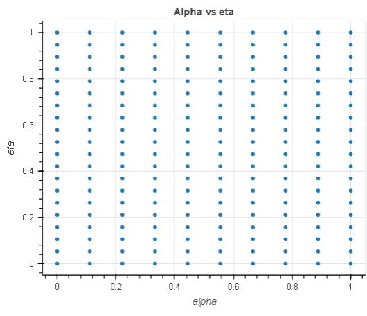 |
The chart to the left shows an analysis of the eta hyperparameter in relation to the objective metric and demonstrates how grid search has exhausted the entire search space (grid) in the X axes before returning the best model. Equally, the chart to the right analyzes the two hyperparameters in a single cartesian space to demonstrate that all the points in the grid were picked during tuning.
The experiment above demonstrates that the exhaustive nature of Grid search guaranties an optimal hyperparameter selection given the defined search space. It also demonstrates that you can reproduce your search result across tuning iterations, all other things being equal.
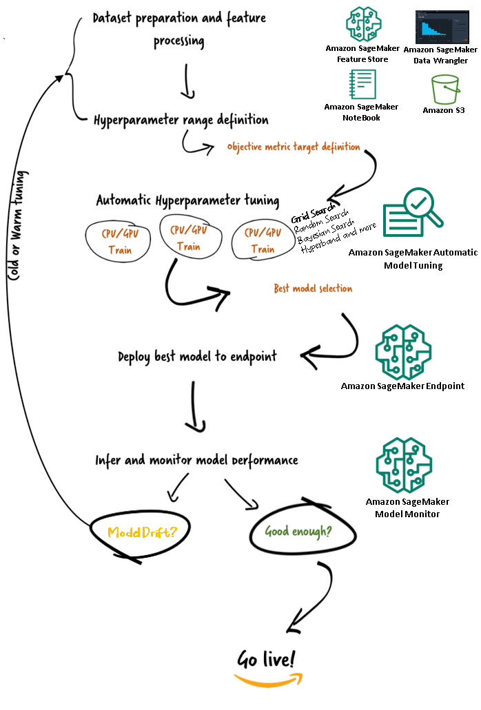
Amazon SageMaker Automatic Model Tuning workflows (AMT)
With Amazon SageMaker automatic model tuning, you can find the best version of your model by running training jobs on your dataset with several search strategies, such as Bayesian, Random search, Grid search, and Hyperband. Automatic model tuning allows you to reduce the time to tune a model by automatically searching for the best hyperparameter configuration within the hyperparameter ranges that you specify.
Now that we have reviewed the advantage of using Grid search in Amazon SageMaker AMT, let’s take a look at AMT’s workflows and understand how it all fits together in SageMaker.
Conclusion
In this post, we discussed how you can now use the Grid search strategy to find the best model and its ability to deterministically reproduce results across different tuning jobs. We discussed the trade-off when using grid search compared to other strategies, and how it allows you to explore what regions of the hyperparameter spaces are most promising and reproduce your results deterministically.
To learn more about automatic model tuning, visit the product page and technical documentation.
About the author
 Doug Mbaya is a Senior Partner Solution architect with a focus in data and analytics. Doug works closely with AWS partners, helping them integrate data and analytics solutions in the cloud.
The breadth of Amazon’s computer vision research is on display at ECCV
Research topics range from visual anomaly detection to road network extraction, regression-constrained neural-architecture search to self-supervised learning for video representations.Read More
Introducing the Amazon SageMaker Serverless Inference Benchmarking Toolkit
Amazon SageMaker Serverless Inference is a purpose-built inference option that makes it easy for you to deploy and scale machine learning (ML) models. It provides a pay-per-use model, which is ideal for services where endpoint invocations are infrequent and unpredictable. Unlike a real-time hosting endpoint, which is backed by a long-running instance, compute resources for serverless endpoints are provisioned on demand, thereby eliminating the need to choose instance types or manage scaling policies.
The following high-level architecture illustrates how a serverless endpoint works. A client invokes an endpoint, which is backed by AWS managed infrastructure.

However, serverless endpoints are prone to cold starts in the order of seconds, and is therefore more suitable for intermittent or unpredictable workloads.
To help determine whether a serverless endpoint is the right deployment option from a cost and performance perspective, we have developed the SageMaker Serverless Inference Benchmarking Toolkit, which tests different endpoint configurations and compares the most optimal one against a comparable real-time hosting instance.
In this post, we introduce the toolkit and provide an overview of its configuration and outputs.
Solution overview
You can download the toolkit and install it from the GitHub repo. Getting started is easy: simply install the library, create a SageMaker model, and provide the name of your model along with a JSON lines formatted file containing a sample set of invocation parameters, including the payload body and content type. A convenience function is provided to convert a list of sample invocation arguments to a JSON lines file or a pickle file for binary payloads such as images, video, or audio.
Install the toolkit
First install the benchmarking library into your Python environment using pip:
You can run the following code from an Amazon SageMaker Studio instance, SageMaker notebook instance, or any instance with programmatic access to AWS and the appropriate AWS Identity and Access Management (IAM) permissions. The requisite IAM permissions are documented in the GitHub repo. For additional guidance and example policies for IAM, refer to How Amazon SageMaker Works with IAM. This code runs a benchmark with a default set of parameters on a model that expects a CSV input with two example records. It’s a good practice to provide a representative set of examples to analyze how the endpoint performs with different input payloads.
Additionally, you can run the benchmark as a SageMaker Processing job, which may be a more reliable option for longer-running benchmarks with a large number of invocations. See the following code:
Note that this will incur additional cost of running an ml.m5.large SageMaker Processing instance for the duration of the benchmark.
Both methods accept a number of parameters to configure, such as a list of memory configurations to benchmark and the number of times each configuration will be invoked. In most cases, the default options should suffice as a starting point, but refer to the GitHub repo for a complete list and descriptions of each parameter.
Benchmarking configuration
Before delving into what the benchmark does and what outputs it produces, it’s important to understand a few key concepts when it comes to configuring serverless endpoints.
There are two key configuration options: MemorySizeInMB and MaxConcurrency. MemorySizeInMB configures the amount of memory that is allocated to the instance, and can be 1024 MB, 2048 MB, 3072 MB, 4096 MB, 5120 MB, or 6144 MB. The number of vCPUs also scales proportionally to the amount of memory allocated. The MaxConcurrency parameter adjusts how many concurrent requests an endpoint is able to service. With a MaxConcurrency of 1, a serverless endpoint can only process a single request at a time.
To summarize, the MemorySizeInMB parameter provides a mechanism for vertical scalability, allowing you to adjust memory and compute resources to serve larger models, whereas MaxConcurrency provides a mechanism for horizontal scalability, allowing your endpoint to process more concurrent requests.
The cost of operating an endpoint is largely determined by the memory size, and there is no cost associated with increasing the max concurrency. However, there is a per-Region account limit for max concurrency across all endpoints. Refer to SageMaker endpoints and quotas for the latest limits.
Benchmarking outputs
Given this, the goal of benchmarking a serverless endpoint is to determine the most cost-effective and reliable memory size setting, and the minimum max concurrency that can handle your expected traffic patterns.
By default, the tool runs two benchmarks. The first is a stability benchmark, which deploys an endpoint for each of the specified memory configurations and invokes each endpoint with the provided sample payloads. The goal of this benchmark is to determine the most effective and stable MemorySizeInMB setting. The benchmark captures the invocation latencies and computes the expected per-invocation cost for each endpoint. It then compares the cost against a similar real-time hosting instance.
When the benchmarking is complete, the tool generates several outputs in the specified result_save_path directory with the following directory structure:
The benchmarking_report directory contains a consolidated report with all the summary outputs that we outline in this post. Additional directories contain raw and intermediate outputs that you can use for additional analyses. Refer to the GitHub repo for a more detailed description of each output artifact.
Let’s examine a few actual benchmarking outputs for an endpoint serving a computer vision MobileNetV2 TensorFlow model. If you’d like to reproduce this example, refer to the example notebooks directory in the GitHub repo.
The first output within the consolidated report is a summary table that provides the minimum, mean, medium, and maximum latency metrics for each MemorySizeInMB successful memory size configuration. As shown in the following table, the average invocation latency (invocation_latency_mean) continued to improve as memory configuration was increased to 3072 MB, but stopped improving thereafter.

In addition to the high-level descriptive statistics, a chart is provided showing the distribution of latency as observed from the client for each of the memory configurations. Again, we can observe that the 1024 MB configuration isn’t as performant as the other options, but there isn’t a substantial difference in performance in configurations of 2048 and above.

Amazon CloudWatch metrics associated with each endpoint configuration are also provided. One key metric here is ModelSetupTime, which measures how long it took to load the model when the endpoint was invoked in a cold state. The metric may not always appear in the report as an endpoint is launched in a warm state. A cold_start_delay parameter is available for specifying the number of seconds to sleep before starting the benchmark on a deployed endpoint. Setting this parameter to a higher number such as 600 seconds should increase the likelihood of a cold state invocation and improve the chances of capturing this metric. Additionally, this metric is far more likely to be captured with the concurrent invocation benchmark, which we discuss later in this section.
The following table shows the metrics captured by CloudWatch for each memory configuration.

The next chart shows the performance and cost trade-offs of different memory configurations. One line shows the estimated cost of invoking the endpoint 1 million times, and the other shows the average response latency. These metrics can inform your decision of which endpoint configuration is most cost-effective. In this example, we see that the average latency flattens out after 2048 MB, whereas the cost continues to increase, indicating that for this model a memory size configuration of 2048 would be most optimal.

The final output of the cost and stability benchmark is a recommended memory configuration, along with a table comparing the cost of operating a serverless endpoint against a comparable SageMaker hosting instance. Based on the data collected, the tool determined that the 2048 MB configuration is the most optimal one for this model. Although the 3072 configuration provides roughly 10 milliseconds better latency, that comes with a 30% increase in cost, from $4.55 to $5.95 per 1 million requests. Additionally, the output shows that a serverless endpoint would provide savings of up to 88.72% against a comparable real-time hosting instance when there are fewer than 1 million monthly invocation requests, and breaks even with a real-time endpoint after 8.5 million requests.

The second type of benchmark is optional and tests various MaxConcurency settings under different traffic patterns. This benchmark is usually run using the optimal MemorySizeInMB configuration from the stability benchmark. The two key parameters for this benchmark is a list of MaxConcurency settings to test along with a list of client multipliers, which determine the number of simulated concurrent clients that the endpoint is tested with.
For example, by setting the concurrency_benchmark_max_conc parameter to [4, 8] and concurrency_num_clients_multiplier to [1, 1.5, 2], two endpoints are launched: one with MaxConcurency of 4 and the other 8. Each endpoint is then benchmarked with a (MaxConcurency x multiplier) number of simulated concurrent clients, which for the endpoint with a concurrency of 4 translates to load test benchmarks with 4, 6, and 8 concurrent clients.
The first output of this benchmark is a table that shows the latency metrics, throttling exceptions, and transactions per second metrics (TPS) associated with each MaxConcurrency configuration with different numbers of concurrent clients. These metrics help determine the appropriate MaxConcurrency setting to handle the expected traffic load. In the following table, we can see that an endpoint configured with a max concurrency of 8 was able to handle up to 16 concurrent clients with only two throttling exceptions out of 2,500 invocations made at an average of 24 transactions per second.

The next set of outputs provides a chart for each MaxConcurrency setting showing the distribution of latency under different loads. In this example, we can see that an endpoint with a MaxConcurrency setting of 4 was able to successfully process all requests with up to 8 concurrent clients with a minimal increase in invocation latency.

The final output provides a table with CloudWatch metrics for each MaxConcurrency configuration. Unlike the previous table showing the distribution of latency for each memory configuration, which may not always display the cold start ModelSetupTime metric, this metric is far more likely to appear in this table due to the larger number of invocation requests and a greater MaxConcurrency.

Conclusion
In this post, we introduced the SageMaker Serverless Inference Benchmarking Toolkit and provided an overview of its configuration and outputs. The tool can help you make a more informed decision with regards to serverless inference by load testing different configurations with realistic traffic patterns. Try the benchmarking toolkit with your own models to see for yourself the performance and cost saving you can expect by deploying a serverless endpoint. Please refer to the GitHub repo for additional documentation and example notebooks.
Additional resources
About the authors
 Simon Zamarin is an AI/ML Solutions Architect whose main focus is helping customers extract value from their data assets. In his spare time, Simon enjoys spending time with family, reading sci-fi, and working on various DIY house projects.
 Dhawal Patel is a Principal Machine Learning Architect at AWS. He has worked with organizations ranging from large enterprises to mid-sized startups on problems related to distributed computing and artificial intelligence. He focuses on deep learning, including NLP and computer vision domains. He helps customers achieve high-performance model inference on SageMaker.
 Rishabh Ray Chaudhury is a Senior Product Manager with Amazon SageMaker, focusing on machine learning inference. He is passionate about innovating and building new experiences for machine learning customers on AWS to help scale their workloads. In his spare time, he enjoys traveling and cooking. You can find him on LinkedIn.