Amazon Lex is a service for building conversational interfaces using voice and text. Amazon Lex provides high-quality speech recognition and language understanding capabilities. With Amazon Lex, you can add sophisticated, natural language bots to new and existing applications. Amazon Lex reduces multi-platform development efforts, allowing you to easily publish your speech or text chatbots to mobile devices and multiple chat services, like Facebook Messenger, Slack, Kik, or Twilio SMS.

Today, we added a Visual Conversation Builder (VCB) to Amazon Lex—a drag-and-drop conversation builder that allows users to interact and define bot information by manipulating visual objects. These are used to design and edit conversation flows in a no-code environment. There are three main benefits of the VCB:

• It’s easier to collaborate through a single pane of glass
• It simplifies conversational design and testing
• It reduces code complexity

In this post, we introduce the VCB, how to use it, and share customer success stories.

Overview of the Visual Conversation Builder

In addition to the already available menu-based editor and Amazon Lex APIs, the visual builder gives a single view of an entire conversation flow in one location, simplifying bot design and reducing dependency on development teams. Conversational designers, UX designers, and product managers—anyone with an interest in building a conversation on Amazon Lex—can utilize the builder.

Designers and developers can now collaborate and build conversations easily in the VCB without coding the business logic behind the conversation. The visual builder helps accelerate time to market for Amazon Lex-based solutions by providing better collaboration, easier iterations of the conversation design, and reduced code complexity.

With the visual builder, it’s now possible to quickly view the entire conversation flow of the intent at a glance and get visual feedback as changes are made. Changes to your design are instantly reflected in the view, and any effects to dependencies or branching logic is immediately apparent to the designer. You can use the visual builder to make any changes to the intent, such as adding utterances, slots, prompts, or responses. Each block type has its own settings that you can configure to tailor the flow of the conversation.

Previously, complex branching of conversations required implementation of AWS Lambda—a serverless, event-driven compute service—to achieve the desired pathing. The visual builder reduces the need for Lambda integrations, and designers can perform conversation branching without the need for Lambda code, as shown in the following example. This helps to decouple conversation design activities from Lambda business logic and integrations. You can still use the existing intent editor in conjunction with the visual builder, or switch between them at any time when creating and modifying intents.

The VCB is a no-code method of designing complex conversations. For example, you can now add a confirmation prompt in an intent and branch based on a Yes or No response to different paths in the flow without code. Where future Lambda business logic is needed, conversation designers can add placeholder blocks into the flow so developers know what needs to be addressed through code. Code hook blocks with no Lambda functions attached automatically take the Success pathway so testing of the flow can continue until the business logic is completed and implemented. In addition to branching, the visual builder offers designers the ability to go to another intent as part of the conversation flow.

Upon saving, VCB automatically scans the build to detect any errors in the conversation flow. In addition, the VCB auto-detects missing failure paths and provides the capability to auto-add those paths into the flow, as shown in the following example.

Using the Visual Conversation Builder

You can access the VCB via the Amazon Lex console by going to a bot and editing or creating a new intent. On the intent page, you can now switch between the visual builder interface and the traditional intent editor, as shown in the following screenshot.

For the intent, the visual builder shows what has already been designed in a visual layout, whereas new intents start with a blank canvas. The visual builder displays existing intents graphically on the canvas. For new intents, you start with a blank canvas and simply drag the components you want to add onto the canvas and begin connecting them together to create the conversation flow.

The visual builder has three main components: blocks, ports, and edges. Let’s get into how these are used in conjunction to create a conversation from beginning to end within an intent.

The basic building unit of a conversation flow is called a block. The top menu of the visual builder contains all the blocks you are able to use. To add a block to a conversation flow, drag it from the top menu onto the flow.

Each block has a specific functionality to handle different use cases of a conversation. The currently available block types are as follows:

• Start – The root or first block of the conversation flow that can also be configured to send an initial response
• Get slot value – Tries to elicit a value for a single slot
• Condition – Can contain up to four custom branches (with conditions) and one default branch
• Dialog code hook – Handles invocation of the dialog Lambda function and includes bot responses based on dialog Lambda functions succeeding, failing, or timing out
• Confirmation – Queries the customer prior to fulfillment of the intent and includes bot responses based on the customer saying yes or no to the confirmation prompt
• Fulfillment – Handles fulfillment of the intent and can be configured to invoke Lambda functions and respond with messages if fulfillment succeeds or fails
• Closing response – Allows the bot to respond with a message before ending the conversation
• Wait for user input – Captures input from the customer and switches to another intent based on the utterance
• End conversation – Indicates the end of the conversation flow

Take the Order Flowers bot as an example. The OrderFlowers intent, when viewed in the visual builder, uses five blocks: Start, three different Get slot value blocks, and Confirmation.

Each block can contain one more ports, which are used to connect one block to another. Blocks contain an input port and one or more output ports based on desired paths for states such a success, timeout, and error.

The connection between the output port of one block and the input port of another block is referred to as an edge.

In the OrderFlowers intent, when the conversation starts, the Start output port is connected to the Get slot value: FlowerType input port using an edge. Each Get slot value block is connected using ports and edges to create a sequence in the conversation flow, which ensures the intent has all the slot values it needs to put in the order.

Notice that currently there is no edge connected to the failure output port of these blocks, but the builder will automatically add these if you choose Save intent and then choose Confirm in the pop-up Auto add block and edges for failure paths. The visual builder then adds an End conversation block and a Go to intent block, connecting the failure and error output ports to Go to intent and connecting the Yes/No ports of the Confirmation block to End conversation.

After the builder adds the blocks and edges, the intent is saved and the conversation flow can be built and tested. Let’s add a Welcome intent to the bot using the visual builder. From the OrderFlowers intent visual builder, choose Back to intents list in the navigation pane. On the Intents page, choose Add intent followed by Add empty intent. In the Intent name field, enter Welcome and choose Add.

Switch to the Visual builder tab and you will see an empty intent, with only the Start block currently on the canvas. To start, add some utterances to this intent so that the bot will be able to direct users to the Welcome intent. Choose the edit button of the Start block and scroll down to Sample utterances. Add the following utterances to this intent and then close the block:

• Can you help me?
• Hi
• Hello
• I need help

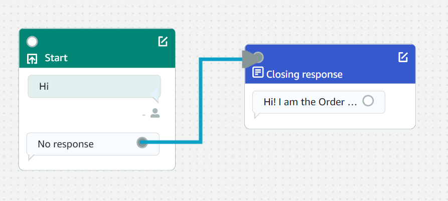
Now let’s add a response for the bot to give when it hits this intent. Because the Welcome intent won’t be processing any logic, we can drag a Closing response block into the canvas to add this message. After you add the block, choose the edit icon on the block and enter the following response:

Hi! I am the Order Flowers Bot. How can I help you today?

The canvas should now have two blocks, but they aren’t connected to each other. We can connect the ports of these two blocks using an edge.

To connect the two ports, simply click and drag from the No response output port of the Start block to the input port of the Closing response block.

At this point, you can complete the conversation flow in two different ways:

• First, you can manually add the End conversation block and connect it to the Closing response block.
• Alternatively, choose Save intent and then choose Confirm to have the builder create this block and connection for you.

After the intent is saved, choose Build and wait for the build to complete, then choose Test.

The bot will now properly greet the customer if an utterance matches this newly created intent.

Customer stories

NeuraFlash is an Advanced AWS Partner with over 40 collective years of experience in the voice and automation space. With a dedicated team of Conversational Experience Designers, Speech Scientists, and AWS developers, NeuraFlash helps customers take advantage of the power of Amazon Lex in their contact centers.

“One of our key focus areas is helping customers leverage AI capabilities for developing conversational interfaces. These interfaces often require specialized bot configuration skills to build effective flows. With the Visual Conversation Builder, our designers can quickly and easily build conversational interfaces, allowing them to experiment at a faster rate and deliver quality products for our customers without requiring developer skills. The drag-and-drop UI and the visual conversation flow is a game-changer for reinventing the contact center experience.”

The SmartBots ML-powered platform lies at the core of the design, prototyping, testing, validating, and deployment of AI-driven chatbots. This platform supports the development of custom enterprise bots that can easily integrate with any application—even an enterprise’s custom application ecosystem.

“The Visual Conversation Builder’s easy-to-use drag-and-drop interface enables us to easily onboard Amazon Lex, and build complex conversational experiences for our customers’ contact centers. With this new functionality, we can improve Interactive Voice Response (IVR) systems faster and with minimal effort. Implementing new technology can be difficult with a steep learning curve, but we found that the drag-and-drop features were easy to understand, allowing us to realize value immediately.“

Conclusion

The Visual Conversation Builder for Amazon Lex is now generally available, for free, in all AWS Regions where Amazon Lex V2 operates.

Additionally, on August 17, 2022, Amazon Lex V2 released a change to the way conversations are managed with the user. This change gives you more control over the path that the user takes through the conversation. For more information, see Understanding conversation flow management. Note that bots created before August 17, 2022, do not support the VCB for creating conversation flows.

To learn more, see Amazon Lex FAQs and the Amazon Lex V2 Developer Guide. Please send feedback to AWS re:Post for Amazon Lex or through your usual AWS support contacts.

About the authors

Thomas Rindfuss is a Sr. Solutions Architect on the Amazon Lex team. He invents, develops, prototypes, and evangelizes new technical features and solutions for Language AI services that improves the customer experience and eases adoption.

Austin Johnson is a Solutions Architect at AWS , helping customers on their cloud journey. He is passionate about building and utilizing conversational AI platforms to add sophisticated, natural language interfaces to their applications.

Read More

“85% of buyers trust online reviews as much as a personal recommendation” – Gartner

Consumers are increasingly engaging with businesses through digital surfaces and multiple touchpoints. Statistics show that the majority of shoppers use reviews to determine what products to buy and which services to use. As per Spiegel Research Centre, the purchase likelihood for a product with five reviews is 270% greater than the purchase likelihood of a product with no reviews. Reviews have the power to influence consumer decisions and strengthen brand value.

In this post, we use Amazon Comprehend to extract meaningful information from product reviews, analyze it to understand how users of different demographics are reacting to products, and discover aggregated information on user affinity towards a product. Amazon Comprehend is a fully managed and continuously trained natural language processing (NLP) service that can extract insight about content of a document or text.

Solution overview

Today, reviews can be provided by customers in various ways, such as star ratings, free text or natural language, or social media shares. Free text or natural language reviews help build trust, as it’s an independent opinion from consumers. It’s often used by product teams to interact with customers through review channels. It’s a proven fact that when customers feel heard, their feeling about the brand improves. Whereas it’s comparatively easier to analyze star ratings or social media shares, natural language or free text reviews pose multiple challenges, like identifying keywords or phrases, topics or concepts, and sentiment or entity-level sentiments. The challenge is mainly due to the variability of length in written text and plausible presence of both signals and noise. Furthermore, the information can either be very clear and explicit (for example, with keywords and key phrases) or unclear and implicit (abstract topics and concepts). Even more challenging is understanding different types of sentiments and relating them to appropriate products and services. Nevertheless, it’s highly critical to understand this information and textual signals in order to provide a frictionless customer experience.

In this post, we use a publicly available NLP – fast.ai dataset to analyze the product reviews provided by customers. We start by using an unsupervised machine learning (ML) technique known as topic modeling. This a popular unsupervised technique that discovers abstract topics that can occur in a text review collection. Topic modeling is a clustering problem that is unsupervised, meaning that the models have no knowledge on possible target variables (such as topics in a review). The topics are represented as clusters. Often, the number of clusters in a corpus of documents is decided with the help of domain experts or by using some standard statistical analysis. The model outputs generally have three components: numbered clusters (topic 0, topic 1, and so on), keywords associated to each cluster, and representative clusters for each document (or review in our case). By its inherent nature, topic models don’t generate human-readable labels for the clusters or topics, which is a common misconception. Something to note about topic modeling in general is that it’s a mixed membership model— every document in the model may have a resemblance to every topic. The topic model learns in an iterative Bayesian process to determine the probability that each document is associated with a given theme or topic. The model output depends on selecting the number of topics optimally. A small number of topics can result in the topics being too broad, and a larger number of topics may result in redundant topics or topics with similarity. There are a number of ways to evaluate topic models:

• Human judgment – Observation-based, interpretation-based
• Quantitative metrics – Perplexity, coherence calculations
• Mixed approach – A combination of judgment-based and quantitative approaches

Perplexity is calculated by splitting a dataset into two parts—a training set and a test set. Likelihood is usually calculated as a logarithm, so this metric is sometimes referred to as the held-out log-likelihood. Perplexity is a predictive metric. It assesses a topic model’s ability to predict a test set after having been trained on a training set. One of the shortcomings of perplexity is that it doesn’t capture context, meaning that it doesn’t capture the relationship between words in a topic or topics in a document. However, the idea of semantic context is important for human understanding. Measures such as the conditional likelihood of the co- occurrence of words in a topic can be helpful. These approaches are collectively referred to as coherence. For this post, we focus on the human judgment (observation-based) approach, namely observing the top n words in a topic.

The solution consists of the following high-level steps:

1. Set up an Amazon SageMaker notebook instance.
2. Create a notebook.
3. Perform exploratory data analysis.
4. Run your Amazon Comprehend topic modeling job.
5. Generate topics and understand sentiment.
6. Use Amazon QuickSight to visualize data and generate reports.

You can use this solution in any AWS Region, but you need to make sure that the Amazon Comprehend APIs and SageMaker are in the same Region. For this post, we use the Region US East (N. Virginia).

Set up your SageMaker notebook instance

You can interact with Amazon Comprehend via the AWS Management Console, AWS Command Line Interface (AWS CLI), or Amazon Comprehend API. For more information, refer to Getting started with Amazon Comprehend. We use a SageMaker notebook and Python (Boto3) code throughout this post to interact with the Amazon Comprehend APIs.

1. On the Amazon SageMaker console, under Notebook in the navigation pane, choose
   Notebook instances.
2. Choose Create notebook instance.
3. Specify a notebook instance name and set the instance type as ml.r5.2xlarge.
4. Leave the rest of the default settings.
5. Create an AWS Identity and Access Management (IAM) role with AmazonSageMakerFullAccess and access to any necessary Amazon Simple Storage Service (Amazon S3) buckets and Amazon Comprehend APIs.
6. Choose Create notebook instance.
   After a few minutes, your notebook instance is ready.
7. To access Amazon Comprehend from the notebook instance, you need to attach the ComprehendFullAccess policy to your IAM role.

For a security overview of Amazon Comprehend, refer to Security in Amazon Comprehend.

Create a notebook

After you open the notebook instance that you provisioned, on the Jupyter console, choose New and then Python 3 (Data Science). Alternatively, you can access the sample code file in the GitHub repo. You can upload the file to the notebook instance to run it directly or clone it.

The GitHub repo contains three notebooks:

• data_processing.ipynb
• model_training.ipynb
• topic_mapping_sentiment_generation.ipynb

Perform exploratory data analysis

We use the first notebook (data_processing.ipynb) to explore and process the data. We start by simply loading the data from an S3 bucket into a DataFrame.

# Bucket containing the data
BUCKET = 'clothing-shoe-jewel-tm-blog'

# Item ratings and metadata
S3_DATA_FILE = 'Clothing_Shoes_and_Jewelry.json.gz' # Zip
S3_META_FILE = 'meta_Clothing_Shoes_and_Jewelry.json.gz' # Zip

S3_DATA = 's3://' + BUCKET + '/' + S3_DATA_FILE
S3_META = 's3://' + BUCKET + '/' + S3_META_FILE

# Transformed review, input for Comprehend
LOCAL_TRANSFORMED_REVIEW = os.path.join('data', 'TransformedReviews.txt')
S3_OUT = 's3://' + BUCKET + '/out/' + 'TransformedReviews.txt'

# Final dataframe where topics and sentiments are going to be joined
S3_FEEDBACK_TOPICS = 's3://' + BUCKET + '/out/' + 'FinalDataframe.csv'

def convert_json_to_df(path):
    """Reads a subset of a json file in a given path in chunks, combines, and returns
    """
    # Creating chunks from 500k data points each of chunk size 10k
    chunks = pd.read_json(path, orient='records', 
                                lines=True, 
                                nrows=500000, 
                                chunksize=10000, 
                                compression='gzip')
    # Creating a single dataframe from all the chunks
    load_df = pd.DataFrame()
    for chunk in chunks:
        load_df = pd.concat([load_df, chunk], axis=0)
    return load_df

# Review data
original_df = convert_json_to_df(S3_DATA)

# Metadata
original_meta = convert_json_to_df(S3_META)

In the following section, we perform exploratory data analysis (EDA) to understand the data. We start by exploring the shape of the data and metadata. For authenticity, we use verified reviews only.

# Shape of reviews and metadata
print('Shape of review data: ', original_df.shape)
print('Shape of metadata: ', original_meta.shape)

# We are interested in verified reviews only
# Also checking the amount of missing values in the review data
print('Frequency of verified/non verified review data: ', original_df['verified'].value_counts())
print('Frequency of missing values in review data: ', original_df.isna().sum())

We further explore the count of each category, and see if any duplicate data is present.

# Count of each categories for EDA.
print('Frequncy of different item categories in metadata: ', original_meta['category'].value_counts())

# Checking null values for metadata
print('Frequency of missing values in metadata: ', original_meta.isna().sum())

# Checking if there are duplicated data. There are indeed duplicated data in the dataframe.
print('Duplicate items in metadata: ', original_meta[original_meta['asin'].duplicated()])

When we’re satisfied with the results, we move to the next step of preprocessing the data. Amazon Comprehend recommends providing at least 1,000 documents in each topic modeling job, with each document at least three sentences long. Documents must be in UTF-8 formatted text files. In the following step, we make sure that data is in the recommended UTF-8 format and each input is no more than 5,000 bytes in size.

def clean_text(df):
    """Preprocessing review text.
    The text becomes Comprehend compatible as a result.
    This is the most important preprocessing step.
    """
    # Encode and decode reviews
    df['reviewText'] = df['reviewText'].str.encode("utf-8", "ignore")
    df['reviewText'] = df['reviewText'].str.decode('ascii')

    # Replacing characters with whitespace
    df['reviewText'] = df['reviewText'].replace(r'r+|n+|t+|u2028',' ', regex=True)

    # Replacing punctuations
    df['reviewText'] = df['reviewText'].str.replace('[^ws]','', regex=True)

    # Lowercasing reviews
    df['reviewText'] = df['reviewText'].str.lower()
    return df

def prepare_input_data(df):
    """Encoding and getting reviews in byte size.
    Review gets encoded to utf-8 format and getting the size of the reviews in bytes. 
    Comprehend requires each review input to be no more than 5000 Bytes
    """
    df['review_size'] = df['reviewText'].apply(lambda x:len(x.encode('utf-8')))
    df = df[(df['review_size'] > 0) & (df['review_size'] < 5000)]
    df = df.drop(columns=['review_size'])
    return df

# Only data points with a verified review will be selected and the review must not be missing
filter = (original_df['verified'] == True) & (~original_df['reviewText'].isna())
filtered_df = original_df[filter]

# Only a subset of fields are selected in this experiment. 
filtered_df = filtered_df[['asin', 'reviewText', 'summary', 'unixReviewTime', 'overall', 'reviewerID']]

# Just in case, once again, dropping data points with missing review text
filtered_df = filtered_df.dropna(subset=['reviewText'])
print('Shape of review data: ', filtered_df.shape)

# Dropping duplicate items from metadata
original_meta = original_meta.drop_duplicates(subset=['asin'])

# Only a subset of fields are selected in this experiment. 
original_meta = original_meta[['asin', 'category', 'title', 'description', 'brand', 'main_cat']]

# Clean reviews using text cleaning pipeline
df = clean_text(filtered_df)

# Dataframe where Comprehend outputs (topics and sentiments) will be added
df = prepare_input_data(df)

We then save the data to Amazon S3 and also keep a local copy in the notebook instance.

# Saving dataframe on S3 df.to_csv(S3_FEEDBACK_TOPICS, index=False) 

# Reviews are transformed per Comprehend guideline- one review per line
# The txt file will be used as input for Comprehend
# We first save the input file locally
with open(LOCAL_TRANSFORMED_REVIEW, "w") as outfile:
    outfile.write("n".join(df['reviewText'].tolist()))

# Transferring the transformed review (input to Comprehend) to S3
!aws s3 mv {LOCAL_TRANSFORMED_REVIEW} {S3_OUT}

This completes our data processing phase.

Run an Amazon Comprehend topic modeling job

We then move to the next phase, where we use the preprocessed data to run a topic modeling job using Amazon Comprehend. At this stage, you can either use the second notebook (model_training.ipynb) or use the Amazon Comprehend console to run the topic modeling job. For instructions on using the console, refer to Running analysis jobs using the console. If you’re using the notebook, you can start by creating an Amazon Comprehend client using Boto3, as shown in the following example.

# Client and session information
session = boto3.Session()
s3 = boto3.resource('s3')

# Account id. Required downstream.
account_id = boto3.client('sts').get_caller_identity().get('Account')

# Initializing Comprehend client
comprehend = boto3.client(service_name='comprehend', 
                          region_name=session.region_name)

You can submit your documents for topic modeling in two ways: one document per file, or one document per line.

We start with 5 topics (k-number), and use one document per line. There is no single best way as a standard practice to select k or the number of topics. You may try out different values of k, and select the one that has the largest likelihood.

# Number of topics set to 5 after having a human-in-the-loop
# This needs to be fully aligned with topicMaps dictionary in the third script 
NUMBER_OF_TOPICS = 5

# Input file format of one review per line
input_doc_format = "ONE_DOC_PER_LINE"

# Role arn (Hard coded, masked)
data_access_role_arn = "arn:aws:iam::XXXXXXXXXXXX:role/service-role/AmazonSageMaker-ExecutionRole-XXXXXXXXXXXXXXX"

Our Amazon Comprehend topic modeling job requires you to pass an InputDataConfig dictionary object with S3, InputFormat, and DocumentReadAction as required parameters. Similarly, you need to provide the OutputDataConfig object with S3 and DataAccessRoleArn as required parameters. For more information, refer to the Boto3 documentation for start_topics_detection_job.

# Constants for S3 bucket and input data file
BUCKET = 'clothing-shoe-jewel-tm-blog'
input_s3_url = 's3://' + BUCKET + '/out/' + 'TransformedReviews.txt'
output_s3_url = 's3://' + BUCKET + '/out/' + 'output/'

# Final dataframe where we will join Comprehend outputs later
S3_FEEDBACK_TOPICS = 's3://' + BUCKET + '/out/' + 'FinalDataframe.csv'

# Local copy of Comprehend output
LOCAL_COMPREHEND_OUTPUT_DIR = os.path.join('comprehend_out', '')
LOCAL_COMPREHEND_OUTPUT_FILE = os.path.join(LOCAL_COMPREHEND_OUTPUT_DIR, 'output.tar.gz')

INPUT_CONFIG={
    # The S3 URI where Comprehend input is placed.
    'S3Uri':    input_s3_url,
    # Document format
    'InputFormat': input_doc_format,
}
OUTPUT_CONFIG={
    # The S3 URI where Comprehend output is placed.
    'S3Uri':    output_s3_url,
}

You can then start an asynchronous topic detection job by passing the number of topics, input configuration object, output configuration object, and an IAM role, as shown in the following example.

# Reading the Comprehend input file just to double check if number of reviews 
# and the number of lines in the input file have an exact match.
obj = s3.Object(input_s3_url)
comprehend_input = obj.get()['Body'].read().decode('utf-8')
comprehend_input_lines = len(comprehend_input.split('n'))

# Reviews where Comprehend outputs will be merged
df = pd.read_csv(S3_FEEDBACK_TOPICS)
review_df_length = df.shape[0]

# The two lengths must be equal
assert comprehend_input_lines == review_df_length

# Start Comprehend topic modelling job.
# Specifies the number of topics, input and output config and IAM role ARN 
# that grants Amazon Comprehend read access to data.
start_topics_detection_job_result = comprehend.start_topics_detection_job(
                                                    NumberOfTopics=NUMBER_OF_TOPICS,
                                                    InputDataConfig=INPUT_CONFIG,
                                                    OutputDataConfig=OUTPUT_CONFIG,
                                                    DataAccessRoleArn=data_access_role_arn)

print('start_topics_detection_job_result: ' + json.dumps(start_topics_detection_job_result))

# Job ID is required downstream for extracting the Comprehend results
job_id = start_topics_detection_job_result["JobId"]
print('job_id: ', job_id)

You can track the current status of the job by calling the DescribeTopicDetectionJob operation. The status of the job can be one of the following:

• SUBMITTED – The job has been received and is queued for processing
• IN_PROGRESS – Amazon Comprehend is processing the job
• COMPLETED – The job was successfully completed and the output is available
• FAILED – The job didn’t complete

# Topic detection takes a while to complete. 
# We can track the current status by calling Use the DescribeTopicDetectionJob operation.
# Keeping track if Comprehend has finished its job
description = comprehend.describe_topics_detection_job(JobId=job_id)

topic_detection_job_status = description['TopicsDetectionJobProperties']["JobStatus"]
print(topic_detection_job_status)
while topic_detection_job_status not in ["COMPLETED", "FAILED"]:
    time.sleep(120)
    topic_detection_job_status = comprehend.describe_topics_detection_job(JobId=job_id)['TopicsDetectionJobProperties']["JobStatus"]
    print(topic_detection_job_status)

topic_detection_job_status = comprehend.describe_topics_detection_job(JobId=job_id)['TopicsDetectionJobProperties']["JobStatus"]
print(topic_detection_job_status)

When the job is successfully complete, it returns a compressed archive containing two files: topic-terms.csv and doc-topics.csv. The first output file, topic-terms.csv, is a list of topics in the collection. For each topic, the list includes, by default, the top terms by topic according to their weight. The second file, doc-topics.csv, lists the documents associated with a topic and the proportion of the document that is concerned with the topic. Because we specified ONE_DOC_PER_LINE earlier in the input_doc_format variable, the document is identified by the file name and the 0-indexed line number within the file. For more information on topic modeling, refer to Topic modeling.
The outputs of Amazon Comprehend are copied locally for our next steps.

# Bucket prefix where model artifacts are stored
prefix = f'{account_id}-TOPICS-{job_id}'

# Model artifact zipped file
artifact_file = 'output.tar.gz'

# Location on S3 where model artifacts are stored
target = f's3://{BUCKET}/out/output/{prefix}/{artifact_file}'

# Copy Comprehend output from S3 to local notebook instance
! aws s3 cp {target}  ./comprehend-out/

# Unzip the Comprehend output file. 
# Two files are now saved locally- 
#       (1) comprehend-out/doc-topics.csv and 
#       (2) comprehend-out/topic-terms.csv

comprehend_tars = tarfile.open(LOCAL_COMPREHEND_OUTPUT_FILE)
comprehend_tars.extractall(LOCAL_COMPREHEND_OUTPUT_DIR)
comprehend_tars.close()

Because the number of topics is much less than the vocabulary associated with the document collection, the topic space representation can be viewed as a dimensionality reduction process as well. You may use this topic space representation of documents to perform clustering. On the other hand, you can analyze the frequency of words in each cluster to determine topic associated with each cluster. For this post, we don’t perform any other techniques like clustering.

Generate topics and understand sentiment

We use the third notebook (topic_mapping_sentiment_generation.ipynb) to find how users of different demographics are reacting to products, and also analyze aggregated information on user affinity towards a particular product.

We can combine the outputs from the previous notebook to get topics and associated terms for each topic. However, the topics are numbered and may lack explainability. Therefore, we prefer to use a human-in-the-loop with enough domain knowledge and subject matter expertise to name the topics by looking at their associated terms. This process can be considered as a mapping from topic numbers to topic names. However, it’s noteworthy that the individual list of terms for the topics can be mutually inclusive and therefore may create multiple mappings. The human-in-the-loop should formalize the mappings based on the context of the use case. Otherwise, the downstream performance may be impacted.

We start by declaring the variables. For each review, there can be multiple topics. We count their frequency and select a maximum of three most frequent topics. These topics are reported as the representative topics of a review. First, we define a variable TOP_TOPICS to hold the maximum number of representative topics. Second, we define and set values to the language_code variable to support the required language parameter of Amazon Comprehend. Finally, we create topicMaps, which is a dictionary that maps topic numbers to topic names.

# boto3 session to access service
session = boto3.Session()
comprehend = boto3.client(  'comprehend',
                            region_name=session.region_name)

# S3 bucket
BUCKET = 'clothing-shoe-jewel-tm-blog'

# Local copy of doc-topic file
DOC_TOPIC_FILE = os.path.join('comprehend-out', 'doc-topics.csv')

# Final dataframe where we will join Comprehend outputs later
S3_FEEDBACK_TOPICS = 's3://' + BUCKET + '/out/' + 'FinalDataframe.csv'

# Final output
S3_FINAL_OUTPUT = 's3://' + BUCKET + '/out/' + 'reviewTopicsSentiments.csv'

# Top 3 topics per product will be aggregated
TOP_TOPICS = 3

# Working on English language only. 
language_code = 'en'

# Topic names for 5 topics created by human-in-the-loop or SME feed
topicMaps = {
    0: 'Product comfortability',
    1: 'Product Quality and Price',
    2: 'Product Size',
    3: 'Product Color',
    4: 'Product Return',
}

Next, we use the topic-terms.csv file generated by Amazon Comprehend to connect the unique terms associated with each topic. Then, by applying the mapping dictionary on this topic-term association, we connect the unique terms to the topic names.

# Loading documents and topics assigned to each of them by Comprehend
docTopics = pd.read_csv(DOC_TOPIC_FILE)
docTopics.head()

# Creating a field with doc number. 
# This doc number is the line number of the input file to Comprehend.
docTopics['doc'] = docTopics['docname'].str.split(':').str[1]
docTopics['doc'] = docTopics['doc'].astype(int)
docTopics.head()

# Load topics and associated terms
topicTerms = pd.read_csv(DOC_TOPIC_FILE)

# Consolidate terms for each topic
aggregatedTerms = topicTerms.groupby('topic')['term'].aggregate(lambda term: term.unique().tolist()).reset_index()

# Sneak peek
aggregatedTerms.head(10)

This mapping improves the readability and explainability of the topics generated by Amazon Comprehend, as we can see in the following DataFrame.

Furthermore, we join the topic number, terms, and names to the initial input data, as shown in the following steps.

This returns topic terms and names corresponding to each review. The topic numbers and terms are joined with each review and then further joined back to the original DataFrame we saved in the first notebook.

# Load final dataframe where Comprehend results will be merged to 
feedbackTopics = pd.read_csv(S3_FEEDBACK_TOPICS)

# Joining topic numbers to main data
# The index of feedbackTopics is referring to doc field of docTopics dataframe
feedbackTopics = pd.merge(feedbackTopics, 
                          docTopics, 
                          left_index=True, 
                          right_on='doc', 
                          how='left')

# Reviews will now have topic numbers, associated terms and topics names
feedbackTopics = feedbackTopics.merge(aggregatedTerms, 
                                      on='topic', 
                                      how='left')
feedbackTopics.head()

We generate sentiment for the review text using detect_sentiment. It inspects text and returns an inference of the prevailing sentiment (POSITIVE, NEUTRAL, MIXED, or NEGATIVE).

def detect_sentiment(text, language_code):
    """Detects sentiment for a given text and language
    """
    comprehend_json_out = comprehend.detect_sentiment(Text=text, LanguageCode=language_code)
    return comprehend_json_out

# Comprehend output for sentiment in raw json 
feedbackTopics['comprehend_sentiment_json_out'] = feedbackTopics['reviewText'].apply(lambda x: detect_sentiment(x, language_code))

# Extracting the exact sentiment from raw Comprehend Json
feedbackTopics['sentiment'] = feedbackTopics['comprehend_sentiment_json_out'].apply(lambda x: x['Sentiment'])

# Sneak peek
feedbackTopics.head(2)

Both topics and sentiments are tightly coupled with reviews. Because we will be aggregating topics and sentiments at product level, we need to create a composite key by combining the topics and sentiments generated by Amazon Comprehend.

# Creating a composite key of topic name and sentiment.
# This is because we are counting frequency of this combination.
feedbackTopics['TopicSentiment'] = feedbackTopics['TopicNames'] + '_' + feedbackTopics['sentiment']

Afterwards, we aggregate at product level and count the composite keys for each product.

This final step helps us better understand the granularity of the reviews per product and categorizing it per topic in an aggregated manner. For instance, we can consider the values shown for topicDF DataFrame. For the first product, of all the reviews for it, overall the customers had a positive experience on product return, size, and comfort. For the second product, the customers had mostly a mixed-to-positive experience on product return and a positive experience on product size.

# Create product id group
asinWiseDF = feedbackTopics.groupby('asin')

# Each product now has a list of topics and sentiment combo (topics can appear multiple times)
topicDF = asinWiseDF['TopicSentiment'].apply(lambda x:list(x)).reset_index()

# Count appreances of topics-sentiment combo for product
topicDF['TopTopics'] = topicDF['TopicSentiment'].apply(Counter)

# Sorting topics-sentiment combo based on their appearance
topicDF['TopTopics'] = topicDF['TopTopics'].apply(lambda x: sorted(x, key=x.get, reverse=True))

# Select Top k topics-sentiment combo for each product/review
topicDF['TopTopics'] = topicDF['TopTopics'].apply(lambda x: x[:TOP_TOPICS])

# Sneak peek
topicDF.head()

Our final DataFrame consists of this topic information and sentiment information joined back to the final DataFrame named feedbackTopics that we saved on Amazon S3 in our first notebook.

# Adding the topic-sentiment combo back to product metadata
finalDF = S3_FEEDBACK_TOPICS.merge(topicDF, on='asin', how='left')

# Only selecting a subset of fields
finalDF = finalDF[['asin', 'TopTopics', 'category', 'title']]

# Saving the final output locally
finalDF.to_csv(S3_FINAL_OUTPUT, index=False)

Use Amazon QuickSight to visualize the data

You can use QuickSight to visualize the data and generate reports. QuickSight is a business intelligence (BI) service that you can use to consume data from many different sources and build intelligent dashboards. In this example, we generate a QuickSight analysis using the final dataset we produced, as shown in the following example visualizations.

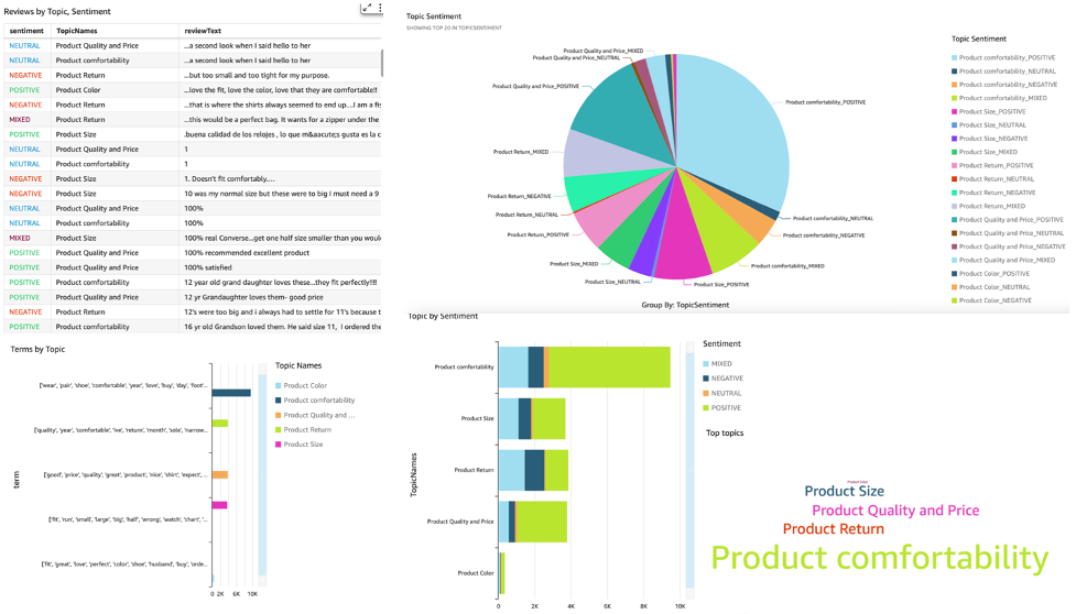
To learn more about Amazon QuickSight, refer to Getting started with Amazon Quicksight.

Cleanup

At the end, we need to shut down the notebook instance we have used in this experiment from AWS Console.

Conclusion

In this post, we demonstrated how to use Amazon Comprehend to analyze product reviews and find the top topics using topic modeling as a technique. Topic modeling enables you to look through multiple topics and organize, understand, and summarize them at scale. You can quickly and easily discover hidden patterns that are present across the data, and then use that insight to make data-driven decisions. You can use topic modeling to solve numerous business problems, such as automatically tagging customer support tickets, routing conversations to the right teams based on topic, detecting the urgency of support tickets, getting better insights from conversations, creating data-driven plans, creating problem-focused content, improving sales strategy, and identifying customer issues and frictions.

These are just a few examples, but you can think of many more business problems that you face in your organization on a daily basis, and how you can use topic modeling with other ML techniques to solve those.

About the Authors

Gurpreet is a Data Scientist with AWS Professional Services based out of Canada. She is passionate about helping customers innovate with Machine Learning and Artificial Intelligence technologies to tap business value and insights from data. In her spare time, she enjoys hiking outdoors and reading books.i

Rushdi Shams is a Data Scientist with AWS Professional Services, Canada. He builds machine learning products for AWS customers. He loves to read and write science fictions.

Wrick Talukdar is a Senior Architect with Amazon Comprehend Service team. He works with AWS customers to help them adopt machine learning on a large scale. Outside of work, he enjoys reading and photography.

Read More

Amazon SageMaker Studio is the first fully integrated development environment (IDE) for machine learning (ML). It provides a single, web-based visual interface where you can perform all ML development steps, including preparing data and building, training, and deploying models.

AWS Glue is a serverless data integration service that makes it easy to discover, prepare, and combine data for analytics, ML, and application development. AWS Glue enables you to seamlessly collect, transform, cleanse, and prepare data for storage in your data lakes and data pipelines using a variety of capabilities, including built-in transforms.

Data engineers and data scientists can now interactively prepare data at scale using their Studio notebook’s built-in integration with serverless Spark sessions managed by AWS Glue. Starting in seconds and automatically stopping compute when idle, AWS Glue interactive sessions provide an on-demand, highly-scalable, serverless Spark backend to achieve scalable data preparation within Studio. Notable benefits of using AWS Glue interactive sessions on Studio notebooks include:

• No clusters to provision or manage
• No idle clusters to pay for
• No up-front configuration required
• No resource contention for the same development environment
• The exact same serverless Spark runtime and platform as AWS Glue extract, transform, and load (ETL) jobs

In this post, we show you how to prepare data at scale in Studio using serverless AWS Glue interactive sessions.

Solution overview

To implement this solution, you complete the following high-level steps:

1. Update your AWS Identity and Access Management (IAM) role permissions.
2. Launch an AWS Glue interactive session kernel.
3. Configure your interactive session.
4. Customize your interactive session and run a scalable data preparation workload.

Update your IAM role permissions

To start, you need to update your Studio user’s IAM execution role with the required permissions. For detailed instructions, refer to Permissions for Glue interactive sessions in SageMaker Studio.

You first add the managed policies to your execution role:

1. On the IAM console, choose Roles in the navigation pane.
2. Find the Studio execution role that you will use, and choose the role name to go to the role summary page.
3. On the Permissions tab, on the Add Permissions menu, choose Attach policies.
4. Select the managed policies AmazonSageMakerFullAccess and AwsGlueSessionUserRestrictedServiceRole
5. Choose Attach policies.
   The summary page shows your newly-added managed policies.Now you add a custom policy and attach it to your execution role.
6. On the Add Permissions menu, choose Create inline policy.
7. On the JSON tab, enter the following policy:

   {
       "Version": "2012-10-17",
       "Statement": [
           {
               "Sid": "VisualEditor0",
               "Effect": "Allow",
               "Action": [
                   "iam:GetRole",
                   "iam:PassRole",
                   "sts:GetCallerIdentity"
               ],
               "Resource": "*"
           }
       ]
   }

8. Modify your role’s trust relationship:

   {
       "Version": "2012-10-17",
       "Statement": [
           {
               "Effect": "Allow",
               "Principal": {
                   "Service": [
                       "glue.amazonaws.com",
                       "sagemaker.amazonaws.com"
                   ]
               },
               "Action": "sts:AssumeRole"
           }
       ]
   }

Launch an AWS Glue interactive session kernel

If you already have existing users within your Studio domain, you may need to have them shut down and restart their Jupyter Server to pick up the new notebook kernel images.

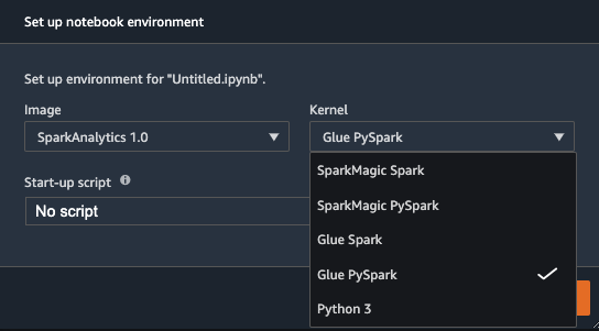
Upon reloading, you can create a new Studio notebook and select your preferred kernel. The built-in SparkAnalytics 1.0 image should now be available, and you can choose your preferred AWS Glue kernel (Glue Scala Spark or Glue PySpark).

Configure your interactive session

You can easily configure your AWS Glue interactive session with notebook cell magics prior to initialization. Magics are small commands prefixed with % at the start of Jupyter cells that provide shortcuts to control the environment. In AWS Glue interactive sessions, magics are used for all configuration needs, including:

• %region – The AWS Region in which to initialize a session. The default is the Studio Region.
• %iam_role – The IAM role ARN to run your session with. The default is the user’s SageMaker execution role.
• %worker_type – The AWS Glue worker type. The default is standard.
• %number_of_workers – The number of workers that are allocated when a job runs. The default is five.
• %idle_timeout – The number of minutes of inactivity after which a session will time out. The default is 2,880 minutes.
• %additional_python_modules – A comma-separated list of additional Python modules to include in your cluster. This can be from PyPi or Amazon Simple Storage Service (Amazon S3).
• %%configure – A JSON-formatted dictionary consisting of AWS Glue-specific configuration parameters for a session.

For a comprehensive list of configurable magic parameters for this kernel, use the %help magic within your notebook.

Your AWS Glue interactive session will not start until the first non-magic cell is run.

Customize your interactive session and run a data preparation workload

As an example, the following notebook cells show how you can customize your AWS Glue interactive session and run a scalable data preparation workload. In this example, we perform an ETL task to aggregate air quality data for a given city, grouping by the hour of the day.

We configure our session to save our Spark logs to an S3 bucket for real-time debugging, which we see later in this post. Be sure that the iam_role that is running your AWS Glue session has write access to the specified S3 bucket.

%help

%session_id_prefix air-analysis-
%glue_version 3.0
%idle_timeout 60
%%configure
{
"--enable-spark-ui": "true",
"--spark-event-logs-path": "s3://<BUCKET>/gis-spark-logs/"
}

Next, we load our dataset directly from Amazon S3. Alternatively, you could load data using your AWS Glue Data Catalog.

from pyspark.sql.functions import split, lower, hour
print(spark.version)
day_to_analyze = "2022-01-05"
df = spark.read.json(f"s3://openaq-fetches/realtime-gzipped/{day_to_analyze}/1641409725.ndjson.gz")
df_air = spark.read.schema(df.schema).json(f"s3://openaq-fetches/realtime-gzipped/{day_to_analyze}/*")

Finally, we write our transformed dataset to an output bucket location that we defined:

df_city = df_air.filter(lower((df_air.city)).contains('delhi')).filter(df_air.parameter == "no2").cache()
df_avg = df_city.withColumn("Hour", hour(df_city.date.utc)).groupBy("Hour").avg("value").withColumnRenamed("avg(value)", "no2_avg")
df_avg.sort("Hour").show()

# Examples of reading / writing to other data stores: 
# https://github.com/aws-samples/aws-glue-samples/tree/master/examples/notebooks

df_avg.write.parquet(f"s3://<BUCKET>/{day_to_analyze}.parquet")

After you’ve completed your work, you can end your AWS Glue interactive session immediately by simply shutting down the Studio notebook kernel, or you could use the %stop_session magic.

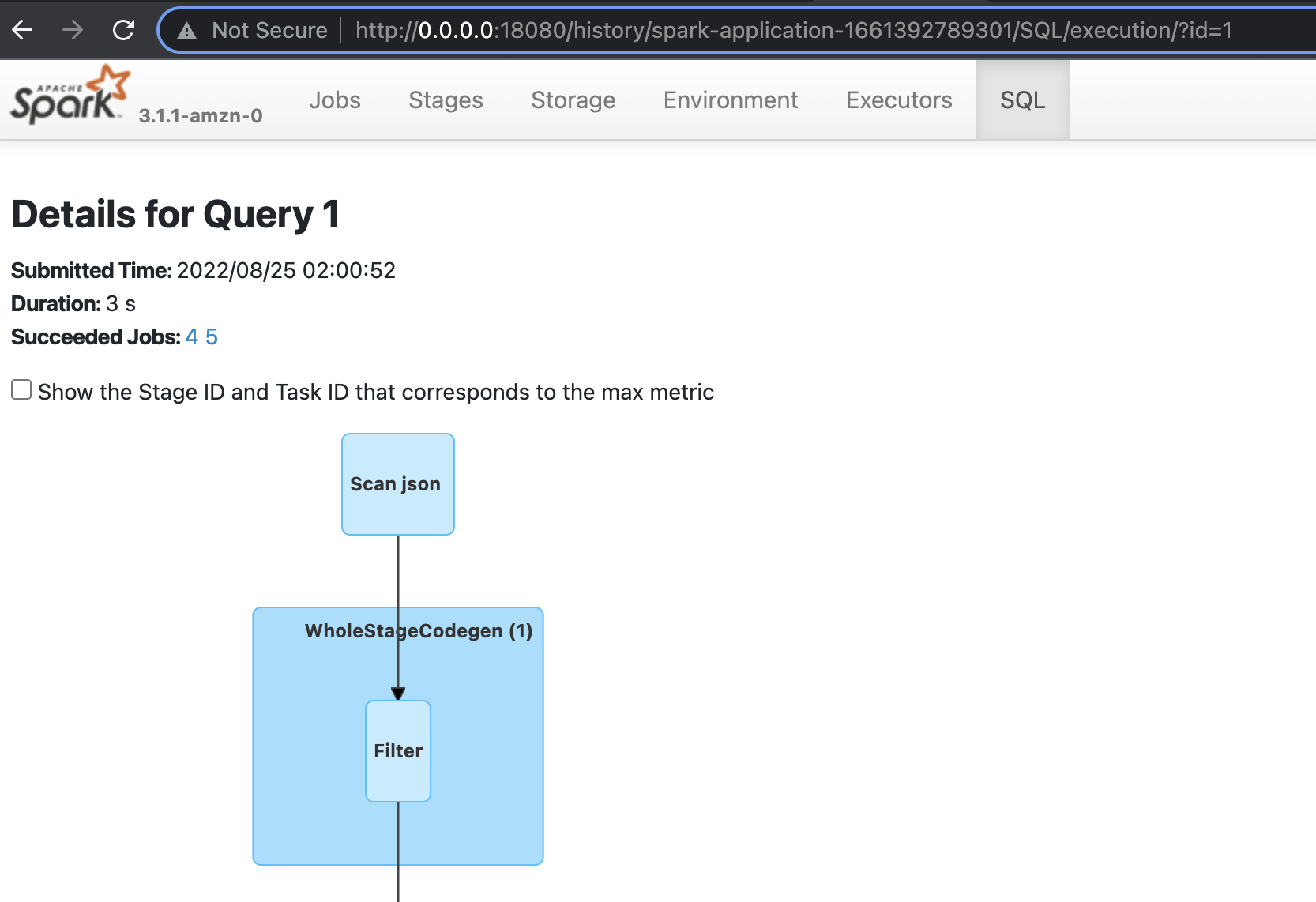
Debugging and Spark UI

In the preceding example, we specified the ”--enable-spark-ui”: “true” argument along with a "--spark-event-logs-path": location. This configures our AWS Glue session to record the sessions logs so that we can utilize a Spark UI to monitor and debug our AWS Glue job in real time.

For the process for launching and reading those Spark logs, refer to Launching the Spark history server. In the following screenshot, we’ve launched a local Docker container that has permission to read the S3 bucket the contains our logs. Optionally, you could host an Amazon Elastic Compute Cloud (Amazon EC2) instance to do this, as described in the preceding linked documentation.

Pricing

When you use AWS Glue interactive sessions on Studio notebooks, you’re charged separately for resource usage on AWS Glue and Studio notebooks.

AWS charges for AWS Glue interactive sessions based on how long the session is active and the number of Data Processing Units (DPUs) used. You’re charged an hourly rate for the number of DPUs used to run your workloads, billed in increments of 1 second. AWS Glue interactive sessions assign a default of 5 DPUs and require a minimum of 2 DPUs. There is also a 1-minute minimum billing duration for each interactive session. To see the AWS Glue rates and pricing examples, or to estimate your costs using the AWS Pricing Calculator, see AWS Glue pricing.

Your Studio notebook runs on an EC2 instance and you’re charged for the instance type you choose, based on the duration of use. Studio assigns you a default EC2 instance type of ml-t3-medium when you select the SparkAnalytics image and associated kernel. You can change the instance type of your Studio notebook to suit your workload. For information about SageMaker Studio pricing, see Amazon SageMaker Pricing.

Conclusion

The native integration of Studio notebooks with AWS Glue interactive sessions facilitates seamless and scalable serverless data preparation for data scientists and data engineers. We encourage you to try out this new functionality in Studio!

See Prepare Data using AWS Glue Interactive Sessions for more information.

About the authors

Sean Morgan is a Senior ML Solutions Architect at AWS. He has experience in the semiconductor and academic research fields, and uses his experience to help customers reach their goals on AWS. In his free time Sean is an activate open source contributor/maintainer and is the special interest group lead for TensorFlow Addons.

Sumedha Swamy is a Principal Product Manager at Amazon Web Services. He leads SageMaker Studio team to build it into the IDE of choice for interactive data science and data engineering workflows. He has spent the past 15 years building customer-obsessed consumer and enterprise products using Machine Learning. In his free time he likes photographing the amazing geology of the American Southwest.

Read More

Register free for NVIDIA GTC to learn from experts on how AI and the evolution of the 3D internet are profoundly impacting industries—and society as a whole. We have prepared several AWS sessions to give you guidance on how to use AWS services powered by NVIDIA technology to meet your goals. Amazon Elastic Compute Cloud (Amazon EC2) instances powered by NVIDIA GPUs deliver the scalable performance needed for fast machine learning (ML) training, cost-effective ML inference, flexible remote virtual workstations, and powerful HPC computations.

AWS is a Global Diamond Sponsor of the conference.

Available sessions

Scaling Deep Learning Training on Amazon EC2 using PyTorch (Presented by Amazon Web Services) [A41454]
As deep learning models grow in size and complexity, they need to be trained using distributed architectures. In this session, we review the details of the PyTorch fully sharded data parallel (FSDP) algorithm, which enables you to train deep learning models at scale.

• Tuesday, September 20, at 2:00 PM – 2:50 PM PDT
• Speakers: Shubha Kumbadakone, Senior GTM Specialist, AWS ML, AWS; and Less Wright, Partner Engineer, Meta

A Developer’s Guide to Choosing the Right GPUs for Deep Learning (Presented by Amazon Web Services) [A41463]
As a deep learning developer or data scientist, choosing the right GPU for deep learning can be challenging. On AWS, you can choose from multiple NVIDIA GPU-based EC2 compute instances depending on your training and deployment requirements. We dive into how to choose the right instance for your needs in this session.

• Available on demand
• Speaker: Shashank Prasanna, Senior Developer Advocate, AI/ML, AWS

Real-time Design in the Cloud with NVIDIA Omniverse on Amazon EC2 (Presented by Amazon Web Services) [A4631]
In this session, we discuss how, by deploying NVIDIA Omniverse Nucleus—the Universal Scene Description (USD) collaboration engine—on EC2 On-Demand compute instances, Omniverse is able to scale to meet the demands of global teams.

• Available on demand
• Speaker: Kellan Cartledge, Spatial Computing Solutions Architect, AWS

5G Killer App: Making Augmented and Virtual Reality a Reality [A41234]
Extended reality (XR), which comprises augmented, virtual, and mixed realities, is consistently envisioned as one of the key killer apps for 5G, because XR requires ultra-low latency and large bandwidths to deliver wired-equivalent experiences for users. In this session, we share how Verizon, AWS, and Ericsson are collaborating to combine 5G and XR technology with NVIDIA GPUs, RTX vWS, and CloudXR to build the infrastructure for commercial XR services across a variety of industries.

• Tuesday, September 20, at 1:00 PM – 1:50 PM PDT
• Speakers: David Randle, Global Head of GTM for Spatial Computing, AWS; Veronica Yip, Product Manager and Product Marketing Manager, NVIDIA; Balaji Raghavachari, Executive Director, Tech Strategy, Verizon; and Peter Linder, Head of 5G Marketing, North America, Ericsson

Accelerate and Scale GNNs with Deep Graph Library and GPUs [A41386]
Graphs play important roles in many applications, including drug discovery, recommender systems, fraud detection, and cybersecurity. Graph neural networks (GNNs) are the current state-of-the-art method for computing graph embeddings in these applications. This session discusses the recent improvements of the Deep Graph Library on NVIDIA GPUs in the DGL 0.9 release cycle.

• Wednesday, September 21, at 2:00 PM – 2:50 PM PDT
• Speaker: Da Zheng, Senior Applied Scientist, AWS

About the author

Jeremy Singh is a Partner Marketing Manager for storage partners within the AWS Partner Network. In his spare time, he enjoys traveling, going to the beach, and spending time with his dog Bolin.

Read More

This post is co-written with Rajnish Jain, Priyanka Kulkarni and Daniel Johnson from Medidata.

Medidata is leading the digital transformation of life sciences, creating hope for millions of patients. Medidata helps generate the evidence and insights to help pharmaceutical, biotech, medical devices, and diagnostics companies as well as academic researchers with accelerating value, minimizing risk, and optimizing outcomes for their solutions. More than one million registered users across over 1,900 customers and partners access the world’s most trusted platform for clinical development, commercial, and real-world data.

Medidata’s AI team combines unparalleled clinical data, advanced analytics, and industry expertise to help life sciences leaders reimagine what is possible, uncover breakthrough insights to make confident decisions, and pursue continuous innovation. Medidata’s AI suite of solutions is backed by an integrated team of scientists, physicians, technologists, and ex-regulatory officials—built upon Medidata’s core platform comprising over 27,000 trials and 8 million patients.

Amazon SageMaker is a fully managed machine learning (ML) platform within the secure AWS landscape. With SageMaker, data scientists and developers can quickly and easily build and train ML models, and then directly deploy them into a production-ready hosted environment. For hosting trained ML models, SageMaker offers a wide array of options. Depending on the type of traffic pattern and latency requirements, you could choose one of these several options. For example, real-time inference is suitable for persistent workloads with millisecond latency requirements, payload sizes up to 6 MB, and processing times of up to 60 seconds. With Serverless Inference, you can quickly deploy ML models for inference without having to configure or manage the underlying infrastructure, and you pay only for the compute capacity used to process inference requests, which is ideal for intermittent workloads. For requests with large unstructured data with payload sizes up to 1 GB, with processing times up to 15 mins, and near real-time latency requirements, you can use asynchronous inference. Batch transform is ideal for offline predictions on large batches of data that are available up front.

In this collaborative post, we demonstrate how AWS helped Medidata take advantage of the various hosting capabilities within SageMaker to experiment with different architecture choices for predicting the operational success of proposed clinical trials. We also validate why Medidata chose SageMaker asynchronous inference for its final design and how this final architecture helped Medidata serve its customers with predictions up to 30 times faster while keeping ML infrastructure costs relatively low.

Architecture evolution

System design is not about choosing one right architecture. It’s the ability to discuss and experiment multiple possible approaches and weigh their trade-offs in satisfying the given requirements for our use case. During this process, it’s essential to take into account prior knowledge of various types of requirements and existing common systems that can interact with our proposed design. The scalability of a system is its ability to easily and cost-effectively vary resources allocated to it so as to serve changes in load. This applies to both increasing or decreasing user numbers or requests to the system.

In the following sections, we discuss how Medidata worked with AWS in iterating over a list of possible scalable architecture designs. We especially focus on the evolution journey, design choices, and trade-offs we went through to arrive at a final choice.

SageMaker batch transform

Medidata originally used SageMaker batch transform for ML inference to meet current requirements and develop a minimum viable product (MVP) for a new predictive solution due to low usage and loose performance requirements of the application. When a batch transform job starts, SageMaker initializes compute instances and distributes the inference or preprocessing workload between them. It’s a high-performance and high-throughput method for transforming data and generating inferences. It’s ideal for scenarios where you’re dealing with large batches of data, don’t need subsecond latency, and need to either preprocess or transform the data or use a trained model to run batch predictions on it in a distributed manner. The Sagemaker batch transform workflow also uses Amazon Simple Storage Service (Amazon S3) as the persistent layer, which maps to one of our data requirements.

Initially, using SageMaker batch transform worked well for the MVP, but as the requirements evolved and Medidata needed to support its customers in near real time, batch transform wasn’t suitable because it was an offline method and customers need to wait anywhere between 5–15 minutes for responses. This primarily included the startup cost for the underlying compute cluster to spin up every time a batch workload needs to be processed. This architecture also required configuring Amazon CloudWatch event rules to track the progress of the batch predictions job together with employing a database of choice to track the states and metadata of the fired job. The MVP architecture is shown in the following diagram.

The flow of this architecture is as follows:

1. The incoming bulk payload is persisted as an input to an S3 location. This event in turn triggers an AWS Lambda Submit function.
2. The Submit function kicks off a SageMaker batch transform job using the SageMaker runtime client.
3. The Submit function also updates a state and metadata tracker database of choice with the job ID and sets the status of the job to inProgress. The function also updates the job ID with its corresponding metadata information.
4. The transient (on-demand) compute cluster required to process the payload spins up, initiating a SageMaker batch transform job. At the same time, the job also emits status notifications and other logging information to CloudWatch logs.
5. The CloudWatch event rule captures the status of the batch transform job and sends a status notification to an Amazon Simple Notification Service (Amazon SNS) topic configured to capture this information.
6. The SNS topic is subscribed by a Notification Lambda function that is triggered every time an event rule is fired by CloudWatch and when there is a message in the SNS topic.
7. The Notification function then updates the status of the transform job for success or failure in the tracking database.

While exploring alternative strategies and architectures, Medidata realized that the traffic pattern for the application consisted of short bursts followed by periods of inactivity. To validate the drawbacks of this existing MVP architecture, Medidata performed some initial benchmarking to understand and prioritize the bottlenecks of this pipeline. As shown in the following diagram, the largest bottleneck was the transition time before running the model for inference due to spinning up new resources with each bulk request. The definition of a bulk request here corresponds to a payload that is a collection of operational site data to be processed rather than a single instance of a request. The second biggest bottleneck was the time to save and write the output, which was also introduced due to the batch model architecture.

As the number of clients increased and usage multiplied, Medidata prioritized user experience by tightening performance requirements. Therefore, Medidata decided to replace the batch transform workflow with a faster alternative. This led to Medidata experimenting with several architecture designs involving SageMaker real-time inference, Lambda, and SageMaker asynchronous inference. In the following sections, we compare these evaluated designs in depth and analyze the technical reasons for choosing one over the other for Medidata’s use case.

SageMaker real-time inference

You can use SageMaker real-time endpoints to serve your models for predictions in real time with low latency. Serving your predictions in real time requires a model serving stack that not only has your trained model, but also a hosting stack to be able to serve those predictions. The hosting stack typically include a type of proxy, a web server that can interact with your loaded serving code, and your trained model. Your model can then be consumed by client applications through a real-time invoke API request. The request payload sent when you invoke the endpoint is routed to a load balancer and then routed to your ML instance or instances that are hosting your models for prediction. SageMaker real-time inference comes with all of the aforementioned components and makes it relatively straightforward to host any type of ML model for synchronous real-time inference.

SageMaker real-time inference has a 60-second timeout for endpoint invocation, and the maximum payload size for invocation is capped out at 6 MB. Because Medidata’s inference logic is complex and frequently requires more than 60 seconds, real-time inference alone can’t be a viable option for dealing with bulk requests that normally require unrolling and processing many individual operational identifiers without re-architecting the existing ML pipeline. Additionally, real-time inference endpoints need to be sized to handle peak load. This could be challenging because Medidata has quick bursts of high traffic. Auto scaling could potentially fix this issue, but it would require manual tuning to ensure there are enough resources to handle all requests at any given time. Alternatively, we could manage a request queue to limit the number of concurrent requests at a given time, but this would introduce additional overhead.

Lambda

Serverless offerings like Lambda eliminate the hassle of provisioning and managing servers, and automatically take care of scaling in response to varying workloads. They can be also much cheaper for lower-volume services because they don’t run 24/7. Lambda works well for workloads that can tolerate cold starts after periods of inactivity. If a serverless function has not been run for approximately 15 minutes, the next request experiences what is known as a cold start because the function’s container must be provisioned.

Medidata built several proof of concept (POC) architecture designs to compare Lambda with other alternatives. As a first simple implementation, the ML inference code was packaged as a Docker image and deployed as a container using Lambda. To facilitate faster predictions with this setup, the invoked Lambda function requires a large provisioned memory footprint. For larger payloads, there is an extra overhead to compress the input before calling the Lambda Docker endpoint. Additional configurations are also needed for the CloudWatch event rules to save the inputs and outputs, tracking the progress of the request, and employing a database of choice to track the internal states and metadata of the fired requests. Additionally, there is also an operational overhead for reading and writing data to Amazon S3. Medidata calculated the projected cost of the Lambda approach based on usage estimates and determined it would be much more expensive than SageMaker with no added benefits.

SageMaker asynchronous inference

Asynchronous inference is one of the newest inference offerings in SageMaker that uses an internal queue for incoming requests and processes them asynchronously. This option is ideal for inferences with large payload sizes (up to 1 GB) or long-processing times (up to 15 minutes) that need to be processed as requests arrive. Asynchronous inference enables you to save on costs by autoscaling the instance count to zero when there are no requests to process, so you only pay when your endpoint is processing requests.

For use cases that can tolerate a cold start penalty of a few minutes, you can optionally scale down the endpoint instance count to zero when there are no outstanding requests and scale back up as new requests arrive so that you only pay for the duration that the endpoints are actively processing requests.

Creating an asynchronous inference endpoint is very similar to creating a real-time endpoint. You can use your existing SageMaker models and only need to specify additional asynchronous inference configuration parameters while creating your endpoint configuration. Additionally, you can attach an auto scaling policy to the endpoint according to your scaling requirements. To invoke the endpoint, you need to place the request payload in Amazon S3 and provide a pointer to the payload as a part of the invocation request. Upon invocation, SageMaker enqueues the request for processing and returns an output location as a response. Upon processing, SageMaker places the inference response in the previously returned Amazon S3 location. You can optionally choose to receive success or error notifications via Amazon SNS.

Based on the different architecture designs discussed previously, we identified several bottlenecks and complexity challenges with these architectures. With the launch of asynchronous inference and based on our extensive experimentation and performance benchmarking, Medidata decided to choose SageMaker asynchronous inference for their final architecture for hosting due to a number of reasons outlined earlier. SageMaker is designed from the ground up to support ML workloads, whereas Lambda is more of a general-purpose tool. For our specific use case and workload type, SageMaker asynchronous inference is cheaper than Lambda. Also, SageMaker asynchronous inference’s timeout is much longer (15 minutes) compared to the real-time inference timeout of 60 seconds. This ensures that asynchronous inference can support all of Medidata’s workloads without modification. Additionally, SageMaker asynchronous inference queues up requests during quick bursts of traffic rather than dropping them, which was a strong requirement as per our use case. Exception and error handling is automatically taken care of for you. Asynchronous inference also makes it easy to handle large payload sizes, which is a common pattern with our inference requirements. The final architecture diagram using SageMaker asynchronous inference is shown in the following figure.

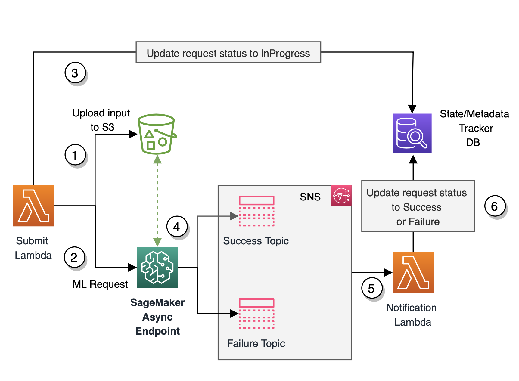
The flow of our final architecture is as follows:

1. The Submit function receives the bulk payload from upstream consumer applications and is set up to be event-driven. This function uploads the payload to the pre-designated Amazon S3 location.
2. The Submit function then invokes the SageMaker asynchronous endpoint, providing it with the Amazon S3 pointer to the uploaded payload.
3. The function also updates the state of the request to inProgress in the state and metadata tracker database.
4. The SageMaker asynchronous inference endpoint reads the input from Amazon S3 and runs the inference logic. When the ML inference succeeds or fails, the inference output is written back to Amazon S3 and the status is sent to an SNS topic.
5. A Notification Lambda function subscribes to the SNS topic. The function is invoked whenever a status update notification is published to the topic.
6. The Notification function updates the status of the request to success or failure in the state and metadata tracker database.

To recap, the batch transform MVP architecture we started with took 5–15 minutes to run depending on the size of the input. With the switch to asynchronous inference, the new solution runs end to end in 10–60 seconds. We see a speedup of at least five times faster for larger inputs and up to 30 times faster for smaller inputs, leading to better customer satisfaction with the performance results. The revised final architecture greatly simplifies the previous asynchronous fan-out/fan-in architecture because we don’t have to worry about partitioning the incoming payload, spawning workers, and delegating and consolidating work amongst the worker Lambda functions.

Conclusion

With SageMaker asynchronous inference, Medidata’s customers using this new predictive application now experience a speedup that’s up to 30 times faster for predictions. Requests aren’t dropped during traffic spikes because the asynchronous inference endpoint queues up requests rather than dropping them. The built-in SNS notification was able to overcome the custom CloudWatch event log notification that Medidata had built to notify the app when the job was complete. In this case, the asynchronous inference approach is cheaper than Lambda. SageMaker asynchronous inference is an excellent option if your team is running heavy ML workloads with burst traffic while trying to minimize cost. This is a great example of collaboration with the AWS team to push the boundaries and use bleeding edge technology for maximum efficiency.

For detailed steps on how to create, invoke, and monitor asynchronous inference endpoints, refer to documentation, which also contains a sample notebook to help you get started. For pricing information, visit Amazon SageMaker Pricing. For examples on using asynchronous inference with unstructured data such as computer vision and natural language processing (NLP), refer to Run computer vision inference on large videos with Amazon SageMaker asynchronous endpoints and Improve high-value research with Hugging Face and Amazon SageMaker asynchronous inference endpoints, respectively.

About the authors

Rajnish Jain is a Senior Director of Engineering at Medidata AI based in NYC. Rajnish heads engineering for a suite of applications that use machine learning on AWS to help customers improve operational success of proposed clinical trials. He is passionate about the use of machine learning to solve business problems.

Priyanka Kulkarni is a Lead Software Engineer within Acorn AI at Medidata Solutions. She architects and develops solutions and infrastructure to support ML predictions at scale. She is a data-driven engineer who believes in building innovative software solutions for customer success.

Daniel Johnson is a Senior Software Engineer within Acorn AI at Medidata Solutions. He builds APIs to support ML predictions around the feasibility of proposed clinical trials.

Arunprasath Shankar is a Senior AI/ML Specialist Solutions Architect with AWS, helping global customers scale their AI solutions effectively and efficiently in the cloud. In his spare time, Arun enjoys watching sci-fi movies and listening to classical music.

Raghu Ramesha is an ML Solutions Architect with the Amazon SageMaker Service team. He focuses on helping customers build, deploy, and migrate ML production workloads to SageMaker at scale. He specializes in machine learning, AI, and computer vision domains, and holds a master’s degree in Computer Science from UT Dallas. In his free time, he enjoys traveling and photography.

Read More

The last few years have seen rapid development in the field of natural language processing (NLP). Although hardware has improved, such as with the latest generation of accelerators from NVIDIA and Amazon, advanced machine learning (ML) practitioners still regularly encounter issues deploying their large language models. Today, we announce new capabilities in Amazon SageMaker that can help: you can configure the maximum Amazon EBS volume size and timeout quotas to facilitate large model inference. Coupled with model parallel inference techniques, you can now use the fully managed model deployment and management capabilities of SageMaker when working with large models with billions of parameters.

In this post, we demonstrate these new SageMaker capabilities by deploying a large, pre-trained NLP model from Hugging Face across multiple GPUs. In particular, we use the Deep Java Library (DJL) serving and tensor parallelism techniques from DeepSpeed to achieve under 0.1 second latency in a text generation use case with 6 billion parameter GPT-J. Complete example on our GitHub repository coming soon.

Large language models and the increasing necessity of model parallel inference

Language models have recently exploded in both size and popularity. In 2018, BERT-large entered the scene and, with its 340 million parameters and novel transformer architecture, set the standard on NLP task accuracy. Within just a few years, state-of-the-art NLP model size has grown by more than 500 times, with models such as OpenAI’s 175 billion parameter GPT-3 and similarly sized open-source Bloom 176 B raising the bar on NLP accuracy. This increase in the number of parameters is driven by the simple and empirically-demonstrated positive relationship between model size and accuracy: more is better. With easy access from model zoos such as Hugging Face and improved accuracy in NLP tasks such as classification and text generation, practitioners are increasingly reaching for these large models. However, deploying them can be a challenge.

Large language models can be difficult to host for low-latency inference use cases because of their size. Typically, ML practitioners simply host a model (or even multiple models) within the memory of a single accelerator device that handles inference end to end on its own. However, large language models can be too big to fit within the memory of a single accelerator, so this paradigm can’t work. For example, open-source GPT-NeoX with 20 billion parameters can require more than 80 GB of accelerator memory, which is more than triple what is available on an NVIDIA A10G, a popular GPU for inference. Practitioners have a few options to work against this accelerator memory constraint. A simple but slow approach is to use CPU memory and stream model parameters sequentially to the accelerator. However, this introduces a communication bottleneck between the CPU and GPU, which can add seconds to inference latency and is therefore unsuitable for many use cases that require fast responses. Another approach is to optimize or compress the model so that it can fit on a single device. Practitioners must implement complex techniques such as quantization, pruning, distillation, and others to reduce the memory requirements. This approach requires a lot of time and expertise and can also reduce the accuracy and generalization of a model, which can also be a non-starter for many use cases.

A third option to use model parallelism. With model parallelism, the parameters and layers of a model are partitioned and then spread across multiple accelerators. This approach allows practitioners to take advantage of both the memory and processing power of multiple accelerators at once and can deliver low-latency inference without impacting the accuracy of the model. Model parallelism is already a popular technique in training (see Introduction to Model Parallelism) and is increasingly becoming used in inference as practitioners require low-latency responses from large models.

There are two general types of model parallelism: pipeline parallelism and tensor parallelism. Pipeline parallelism splits a model between layers, so that any given layer is contained within the memory of a single GPU. In contrast, tensor parallelism splits layers such that a model layer is spread out across multiple GPUs. Both of these model parallel techniques are used in training (often together), but tensor parallelism can be a better choice for inference because batch size is often one with inference. When batch size is one, only tensor parallelism can take advantage of multiple GPUs at once when processing the forward pass to improve latency.

In this post, we use DeepSpeed to partition the model using tensor parallelism techniques. DeepSpeed Inference supports large Transformer-based models with billions of parameters. It allows you to efficiently serve large models by adapting to the best parallelism strategies for multi-GPU inference, accounting for both inference latency and cost. For more information, refer to DeepSpeed: Accelerating large-scale model inference and training via system optimizations and compression and this DeepSpeed Inference: Enabling Efficient Inference of Transformer Models at Unprecedented Scale.

Solution overview

The Deep Java Library (DJL) is an open-source, high-level, engine-agnostic Java framework for deep learning. The DJL is built with native Java concepts on top of existing deep learning frameworks. The DJL is designed to be deep learning engine agonistic. You can switch engines at any point. The DJL also provides automatic CPU/GPU choice based on hardware configuration.

Although the DJL is designed originally for Java developers to get start with ML, DJLServing is a high-performance universal model serving solution powered by the DJL that is programming language agnostic. It can serve the commonly seen model types, such the PyTorch TorchScript model, TensorFlow SavedModel bundle, Apache MXNet model, ONNX model, TensorRT model, and Python script model. DJLServing supports dynamic batching and worker auto scaling to increase throughput. You can load different versions of a model on a single endpoint. You can also serve models from different ML frameworks at the same time. What’s more, DJLServing natively supports multi-GPU by setting up MPI configurations and socket connections for inference. This frees the heavy lifting of setting up a multi-GPU environment.

Our proposed solution uses the newly announced SageMaker capabilities, DJLServing and DeepSpeed Inference, for large model inference. As of this writing, all Transformer-based models are supported. This solution is intended for parallel model inference using a single model on a single instance.

DJLServing is built with multiple layers. The routing layer is built on top of Netty. The remote requests are handled in the routing layer to distribute to workers, either threads in Java or processes in Python, to run inference. The total number of Java threads are set to 2 * cpu_core from the machine to make full usage of computing power. The worker numbers can be configured per model or the DJL’s auto-detection on hardware. The following diagram illustrates our architecture.

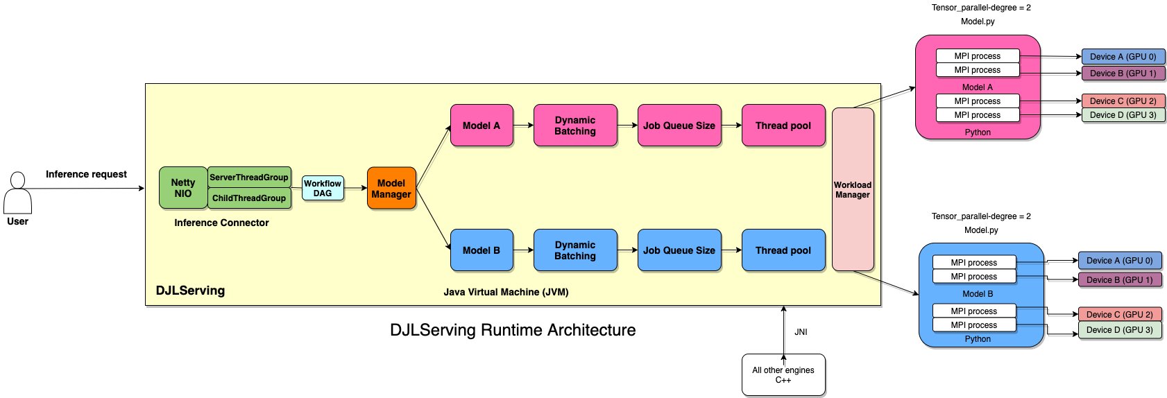
Inference large models on SageMaker

The following steps demonstrate how to deploy a gpt-j-6B model in SageMaker using DJL serving. This is made possible by the capability to configure the EBS volume size, model download timeout time, and startup health-check timeout time. You can try out this demo by running the following notebook.

Pull the Docker image and push to Amazon ECR

The Docker image djl-serving:0.18.0-deepspeed is our DJL serving container with DeepSpeed incorporated. We then push this image to Amazon Elastic Container Registry (Amazon ECR) for later use. See the following code:

docker pull deepjavalibrary/djl-serving:0.18.0-deepspeed

Create our model file

First, we create a file called serving.properties that contains only one line of code. This tells the DJL model server to use the Rubikon engine. Rubikon is an AWS developed large model supporting package. In this demo, it facilitates the MPI threads setup and socket connection. It also sets the number of GPUs (model slicing number) by reading in the TENSOR_PARALLEL_DEGREE parameter defined in our model.py file in the next paragraph. The file contains the following code:

engine=Rubikon

Next, we create our model.py file, which defines our model as gpt-j-6B. In our code, we read in the TENSOR_PARALLEL_DEGREE environment variable (default value is 1). This sets the number of devices over which the tensor parallel modules are distributed. Please note, DeepSpeed provides a few built-in partition logics, and gpt-j-6B is one of them. We use it by specifying replace_method and relpace_with_kernel_inject. If you have your customized model and need DeepSpeed to partition effectively, you need to change relpace_with_kernel_inject to false and add injection_policy to make the runtime partition work. For more information, refer to Initializing for Inference.

from djl_python import Input, Output
import os
import deepspeed
import torch
from transformers import pipeline, AutoModelForCausalLM, AutoTokenizer

predictor = None

def get_model():
    model_name = 'EleutherAI/gpt-j-6B'
    tensor_parallel = int(os.getenv('TENSOR_PARALLEL_DEGREE', '1'))
    local_rank = int(os.getenv('LOCAL_RANK', '0'))
    model = AutoModelForCausalLM.from_pretrained(model_name, revision="float32", torch_dtype=torch.float32)
    tokenizer = AutoTokenizer.from_pretrained(model_name)
    
    model = deepspeed.init_inference(model,
                                     mp_size=tensor_parallel,
                                     dtype=model.dtype,
                                     replace_method='auto',
                                     replace_with_kernel_inject=True)
    generator = pipeline(task='text-generation', model=model, tokenizer=tokenizer, device=local_rank)
    return generator


def handle(inputs: Input) -> None:
    global predictor
    if not predictor:
        predictor = get_model()

    if inputs.is_empty():
        # Model server makes an empty call to warmup the model on startup
        return None

    data = inputs.get_as_string()
    result = predictor(data, do_sample=True, min_tokens=200, max_new_tokens=256)
    return Output().add(result)

We create a directory called gpt-j and copy model.py and serving.properties to this directory:

mkdir gpt-j
cp model.py gpt-j
cp serving.properties gpt-j

Lastly, we create the model file and upload it to Amazon Simple Storage Service (Amazon S3):

tar cvfz gpt-j.tar.gz gpt-j
aws s3 cp gpt-j.tar.gz s3://djl-sm-test/deepspeed/

Create a SageMaker model

We now create a SageMaker model. We use the ECR image we created earlier and the model artifact from the previous step to create the SageMaker model. In the model setup, we configure TENSOR_PARALLEL_DEGREE=2, which means the model will be partitioned along 2 GPUs. See the following code:

aws sagemaker create-model 
--model-name gpt-j 
--primary-container 
Image=<account_id>.dkr.ecr.us-east-1.amazonaws.com/djl-deepspeed:latest,ModelDataUrl=s3://djl-sm-test/deepspeed/gpt-j.tar.gz,Environment={TENSOR_PARALLEL_DEGREE=2} 
--execution-role-arn <IAM_role_arn>

After running the preceding command, you see output similar to the following:

{
    "ModelArn": "arn:aws:sagemaker:us-east-1:<account_id>:model/gpt-j"
}

Create a SageMaker endpoint

You can use any instances with multiple GPUs for testing. In this demo, we use a p3.16xlarge instance. In the following code, note how we set the ModelDataDownloadTimeoutInSeconds, ContainerStartupHealthCheckTimeoutInSeconds, and VolumeSizeInGB parameters to accommodate the large model size. The VolumeSizeInGB parameter is applicable to GPU instances supporting the EBS volume attachment.

aws sagemaker create-endpoint-config 
    --region us-east-1 
    --endpoint-config-name gpt-j-config 
    --production-variants '[
      {
        "ModelName": "gpt-j",
        "VariantName": "AllTraffic",
        "InstanceType": "ml.p3.16xlarge",
        "InitialInstanceCount": 1,
        "VolumeSizeInGB": 256,
        "ModelDataDownloadTimeoutInSeconds": 1800,
        "ContainerStartupHealthCheckTimeoutInSeconds": 3600
        }
    ]'

Lastly, we create a SageMaker endpoint:

aws sagemaker create-endpoint 
--endpoint-name gpt-j 
--endpoint-config-name gpt-j-config

You see it printed out in the following code:

{
    "EndpointArn": "arn:aws:sagemaker:us-east-1:<aws-account-id>:endpoint/gpt-j"
}

Starting the endpoint might take a while. You can try a few more times if you run into the InsufficientInstanceCapacity error.

Performance tuning

Performance tuning and optimization is an empirical process often involving multiple iterations. The number of parameters to tune is combinatorial and the set of configuration parameter values aren’t independent of each other. Various factors affect optimal parameter tuning, including payload size, type, and the number of ML models in the inference request flow graph, storage type, compute instance type, network infrastructure, application code, inference serving software runtime and configuration, and more.

SageMaker real-time inference is ideal for inference workloads where you have real-time, interactive, low-latency requirements. There are four most commonly used metrics for monitoring inference request latency for SageMaker inference endpoints:

• Container latency – The time it takes to send the request, fetch the response from the model’s container, and complete inference in the container. This metric is available in Amazon CloudWatch as part of the invocation metrics published by SageMaker.
• Model latency – The total time taken by all SageMaker containers in an inference pipeline. This metric is available in CloudWatch as part of the invocation metrics published by SageMaker.
• Overhead latency – Measured from the time that SageMaker receives the request until it returns a response to the client, minus the model latency. This metric is available in CloudWatch as part of the invocation metrics published by SageMaker.
• End-to-end latency – Measured from the time the client sends the inference request until it receives a response back. You can publish this as a custom metric in CloudWatch.

Container latency depends on several factors; the following are among the most important:

• Underlying protocol (HTTP(s)/gRPC) used to communicate with the inference server
• Overhead related to creating new TLS connections
• Deserialization time of the request/response payload
• Request queuing and batching features provided by the underlying inference server
• Request scheduling capabilities provided by the underlying inference server
• Underlying runtime performance of the inference server
• Performance of preprocessing and postprocessing libraries before calling the model prediction function
• Underlying ML framework backend performance
• Model-specific and hardware-specific optimizations

In this section, we focus primarily on container latency and specifically on optimizing DJLServing running inside a SageMaker container.

Tune the ML engine for multi-threaded inference

One of the advantages of the DJL is multi-threaded inference support. It can help increase the throughput of your inference on multi-core CPUs and GPUs and reduce memory consumption compare to Python. Refer to Inference Performance Optimization for more information about optimizing the number of threads for different engines.

Tune Netty

DJLServing is built with multiple layers. The routing layer is built on top of Netty. Netty is a NIO client server framework that enables quick and easy development of network applications such as protocol servers and clients. In Netty, Channel is the main container; it contains a ChannelPipeline and is associated with an EventLoop (a container for a thread) from an EventLoopGroup. EventLoop is essentially an I/O thread and may be shared by multiple channels. ChannelHandlers are run on these EventLoop threads. This simple threading model means that you don’t need to worry about concurrency issues in the run of your ChannelHandlers. You are always guaranteed sequential runs on the same thread for a single run through your pipeline. DJLServing uses Netty’s EpollEventLoopGroup on Linux. The total number of Netty threads by default is set to 2 * the number of virtual CPUs from the machine to make full usage of computing power. Furthermore, because you don’t create large numbers of threads, your CPU isn’t overburdened by context switching. This default setting works fine in most cases; however, if you want to set the number of Netty threads for processing the incoming requests, you can do so by setting the SERVING_NUMBER_OF_NETTY_THREADS environment variable.

Tune workload management (WLM) of DJLServing

DJLServing has WorkLoadManager, which is responsible for managing the workload of the worker thread. It manages the thread pools and job queues, and scales up or down the required amount of worker threads per ML model. It has auto scaling, which adds an inference job to the job queue of the next free worker and scales up the worker thread pool for that specific model if necessary. The scaling is primarily based on the job queue depth of the model, the batch size, and the current number of worker threads in the pool. The job_queue_size controls the number of inference jobs that can be queued up at any point in time. By default, it is set to 100. If you have higher concurrency needs per model serving instance, you can increase the job_queue_size, thread pool size, and minimum or maximum thread workers for a particular model by setting the properties in serving.properties, as shown in the following example code:

serving.properties
# use minWorkers/maxWorkers for all devices
gpu.minWorkers=2
gpu.maxWorkers=3
cpu.minWorkers=2
cpu.maxWorkers=4

As of this writing, you can’t configure job_queue_size in serving.properties. The default value job_queue_size is controlled by an environment variable, and you can only configure the per-model setting with the registerModel API.

Many practitioners tend to run inference sequentially when the server is invoked with multiple independent requests. Although easier to set up, it’s usually not the best practice to utilize GPU’s compute power. To address this, DJLServing offers the built-in optimizations of dynamic batching to combine these independent inference requests on the server side to form a larger batch dynamically to increase throughput.

All the requests reach the dynamic batcher first before entering the actual job queues to wait for inference. You can set your preferred batch sizes for dynamic batching using the batch_size settings in serving.properties. You can also configure max_batch_delay to specify the maximum delay time in the batcher to wait for other requests to join the batch based on your latency requirements.

You can fine-tune the following parameters to increase the throughput per model:

• batch_size – The inference batch size. The default value is 1.
• max_batch_delay – The maximum delay for batch aggregation. The default value is 100 milliseconds.
• max_idle_time – The maximum idle time before the worker thread is scaled down.
• min_worker – The minimum number of worker processes. For the DJL’s DeepSpeed engine, min_worker is set to number of GPUs/TENSOR_PARALLEL_DEGREE.
• max_worker – The maximum number of worker processes. For the DJL’s DeepSpeed engine, max_worker is set to mumber of GPUs/TENSOR_PARALLEL_DEGREE.

Tune degree of tensor parallelism

For large model support that doesn’t fit in the single accelerator device memory, the number of Python processes are determined by the total number of accelerator devices on the host. The tensor_parallel_degree is created for slicing the model and distribute to multiple accelerator devices. In this case, even if a model is too large to host on a single accelerator, it can still be handled by DJLServing and can run on multiple accelerator devices by partitioning the model. Internally, DJLServing creates multiple MPI processes (equal to tensor_parallel_degree) to manage the slice of each model on each accelerator device.

You can set the number of partitions for your model by setting the TENSOR_PARALLEL_DEGREE environment variable. Please note this configuration is a global setting and applies to all the models on the host. If the TENSOR_PARALLEL_DEGREE is less than the total number of accelerator devices (GPUs), DJLServing launches multiple Python process groups equivalent to the total number of GPUs/TENSOR_PARALLEL_DEGREE. Each Python process group consists of Python processes equivalent to TENSOR_PARALLEL_DEGREE. Each Python process group holds the full copy of the model.

Summary

In this post, we showcased the newly launched SageMaker capability to allow you to configure inference instance EBS volumes, model downloading timeout, and container startup timeout. We demonstrated this new capability in an example of deploying a large model in SageMaker. We also covered options available to tune the performance of the DJL. For more details about SageMaker and the new capability launched, refer to [!Link] and [!Link].

About the authors

Frank Liu is a Software Engineer for AWS Deep Learning. He focuses on building innovative deep learning tools for software engineers and scientists. In his spare time, he enjoys hiking with friends and family.

Qing Lan is a Software Development Engineer in AWS. He has been working on several challenging products in Amazon, including high performance ML inference solutions and high performance logging system. Qing’s team successfully launched the first Billion-parameter model in Amazon Advertising with very low latency required. Qing has in-depth knowledge on the infrastructure optimization and Deep Learning acceleration.

Qingwei Li is a Machine Learning Specialist at Amazon Web Services. He received his Ph.D. in Operations Research after he broke his advisor’s research grant account and failed to deliver the Nobel Prize he promised. Currently he helps customers in the financial service and insurance industry build machine learning solutions on AWS. In his spare time, he likes reading and teaching.

Dhawal Patel is a Principal Machine Learning Architect at AWS. He has worked with organizations ranging from large enterprises to mid-sized startups on problems related to distributed computing, and Artificial Intelligence. He focuses on Deep learning including NLP and Computer Vision domains. He helps customers achieve high performance model inference on SageMaker.

Robert Van Dusen is a Senior Product Manager at AWS.

Alan Tan is a Senior Product Manager with SageMaker leading efforts on large model inference. He’s passionate about applying Machine Learning to the area of Analytics. Outside of work, he enjoys the outdoors.

Read More