This is a guest blog post cowritten with athenahealth.
athenahealth a leading provider of network-enabled software and services for medical groups and health systems nationwide. Its electronic health records, revenue cycle management, and patient engagement tools allow anytime, anywhere access, driving better financial outcomes for its customers and enabling its provider customers to deliver better quality care.
In the artificial intelligence (AI) space, athenahealth uses data science and machine learning (ML) to accelerate business processes and provide recommendations, predictions, and insights across multiple services. From its first implementation in automated document services, touchlessly processing millions of provider-patient documents, to its more recent work in virtual assistants and improving revenue cycle performance, athenahealth continues to apply AI to help drive efficiency, service capabilities, and better outcomes for providers and their patients.
This blog post demonstrates how athenahealth uses Kubeflow on AWS (an AWS-specific distribution of Kubeflow) to build and streamline an end-to-end data science workflow that preserves essential tooling, optimizes operational efficiency, increases data scientist productivity, and sets the stage for extending their ML capabilities more easily.
Kubeflow is the open-source ML platform dedicated to making deployments of ML workflows on Kubernetes simple, portable, and scalable. Kubeflow achieves this by incorporating relevant open-source tools that integrate well with Kubernetes. Some of these projects include Argo for pipeline orchestration, Istio for service mesh, Jupyter for notebooks, Spark, TensorBoard, and Katib. Kubeflow Pipelines helps build and deploy portable, scalable ML workflows that can include steps like data extraction, preprocessing, model training, and model evaluation in the form of repeatable pipelines.
AWS is contributing to the open-source Kubeflow community by providing its own Kubeflow distribution (called Kubeflow on AWS) that helps organizations like athenahealth build highly reliable, secure, portable, and scalable ML workflows with reduced operational overhead through integration with AWS managed services. AWS provides various Kubeflow deployment options like deployment with Amazon Cognito, deployment with Amazon Relational Database Service (Amazon RDS) and Amazon Simple Storage Service (Amazon S3), and vanilla deployment. For details on service integration and available add-ons for each of these options, refer to Deployment.
Today, Kubeflow on AWS provides a clear path to using Kubeflow, augmented with the following AWS services:
Many AWS customers are taking advantage of the Kubeflow on AWS distribution, including athenahealth.
Here, the athenahealth MLOps team discuss the challenges they encountered and the solutions they created in their Kubeflow journey.
Challenges with the previous ML environment
Prior to our adoption of Kubeflow on AWS, our data scientists used a standardized set of tools and a process that allowed flexibility in the technology and workflow used to train a given model. Example components of the standardized tooling include a data ingestion API, security scanning tools, the CI/CD pipeline built and maintained by another team within athenahealth, and a common serving platform built and maintained by the MLOps team. However, as our use of AI and ML matured, the variety of tools and infrastructure created for each model grew. Although we were still able to support the existing process, we saw the following challenges on the horizon:
-
Maintenance and growth – Reproducing and maintaining model training environments took more effort as the number of deployed models increased. Each project maintained detailed documentation that outlined how each script was used to build the final model. In many cases, this was an elaborate process involving 5 to 10 scripts with several outputs each. These had to be manually tracked with detailed instructions on how each output would be used in subsequent processes. Maintaining this over time became cumbersome. Moreover, as the projects became more complex, the number of tools also increased. For example, most models utilized Spark and TensorFlow with GPUs, which required a larger variety of environment configurations. Over time, users would switch to newer versions of tools in their development environments but then couldn’t run older scripts when those versions became incompatible. Consequently, maintaining and augmenting older projects required more engineering time and effort. In addition, as new data scientists joined the team, knowledge transfers and onboarding took more time, because synchronizing local environments included many undocumented dependencies. Switching between projects faced the same issues because each model had its own workflows.
-
Security – We take security seriously, and therefore prioritize compliance with all contractual, legal, and regulatory obligations associated with ML and data science. Data must be utilized, stored, and accessed in specific ways, and we have embedded robust processes to ensure our practices comply with our legal obligations as well as align with industry best practices. Prior to Kubeflow adoption, ensuring that data was stored and accessed in a specific way involved regular verification across multiple, diverse workflows. We knew that we could improve efficiencies by consolidating these diverse workflows onto a single platform. However, that platform would need to be flexible enough to integrate well with our standardized tooling.
-
Operations – We also saw an opportunity to increase operational efficiency and management through centralizing the logging and monitoring of the workflows. Because each team had developed their own tools, we collected this information from each workflow individually and aggregated them.
The data science team evaluated various solutions for consolidating the workflows. In addition to addressing these requirements, we looked for a solution that would integrate seamlessly with the existing standardized infrastructure and tools. We selected Amazon EKS and Kubeflow on AWS as our workflow solution.
The data scientist development cycle incorporating Kubeflow
A data science project begins with a clean slate: no data, no code, only the business problem that can be solved with ML. The first task is a proof of concept (POC) to discover if the data holds enough signal to make an ML model effective at solving the business problem, starting with querying for the raw dataset from our Snowflake data warehouse. This stage is iterative, and the data scientists use Kubernetes pods or Kubeflow Jupyter notebooks during this process.
Our Kubeflow cluster uses the Karpenter cluster autoscaler, which makes spinning up resources easy for data scientists because they only need to focus on defining the desired instance types, while the provisioning work is done by a set of predefined Karpenter provisioners. We have separate provisioners for CPU and GPU instance types, and all the instances supported by Amazon EKS fall in one of these two categories as per our provisioner configuration. The data scientists choose instance types using node selectors, and Karpenter takes care of node lifecycle management.
After the query is developed, the data scientists extract the raw data to a location on Amazon S3, then launch a Jupyter notebook from the AWS Kubeflow UI to explore the data. The goal is to create the feature set that will be used to train the first model. This allows the data scientists to determine if there is enough signal in the data to fulfill the customer’s business need.
After the results are satisfactory, the data scientists move to the next stage of the development cycle and turn their discoveries into a robust pipeline. They convert the POC code into production-quality code that runs at scale. To ensure compliance through using approved libraries, a container is created with the appropriate base Docker image. For our data scientists, we have found that providing a standard Python, TensorFlow, and Spark base image gives sufficient flexibility for most, if not all, workloads. They can then use the Dockerfile of their component to further customize their development environment. This Dockerfile is then utilized by the CI/CD process to build the components image that will be used in production, therefore maintaining consistency between development and production environments.
We have a tool that gives data scientists the ability to launch their development environment in a pod running on Kubernetes. When this pod is running, the data scientists can then attach the Visual Studio Code IDE directly to the pod and debug their model code. After they have the code running successfully, they can then push their changes to git and a new development environment is created with the most recent changes.
The standard data science pipeline consists of stages that include extraction, preprocessing, training, and evaluation. Each stage in the pipeline appears as a component in Kubeflow, which consists of a Kubernetes pod that runs a command with some information passed in as parameters. These parameters can either be static values or references to output from a previous component. The Docker image used in the pod is built from the CI/CD process. Details on this process appear in the CI/CD workflow discussed in the next section.
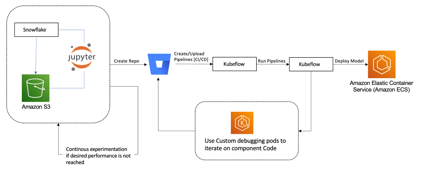
Development Cycle on Kubeflow. The development workflow starts on the left with the POC. The completed model is deployed to the athenahealth model serving platform running on Amazon ECS.
CI/CD process supporting automated workflows
As part of our CI/CD process, we use Jenkins to build and test all Kubeflow component images in parallel. On successful completion, the pipeline component template contains reference pointers to the images, and the resulting pipeline is uploaded to Kubeflow. Parameters in the Jenkins pipeline allow users to launch the pipelines and run their model training tests after successful builds.
Alternatively, to maintain a short development cycle, data scientists can also launch the pipeline from their local machine, modifying any pipeline parameters they may be experimenting with.
Tooling exists to ensure the reference pointers from the CI/CD build are utilized by default. If there is a deployable artifact in the repo, then the CI/CD logic will continue to deploy the artifact to the athenahealth model serving platform (the Prediction Service) running on Amazon ECS with AWS Fargate. After all these stages have passed, the data scientist merges the code to the primary branch. The pipelines and deployable artifacts are then pushed to production.
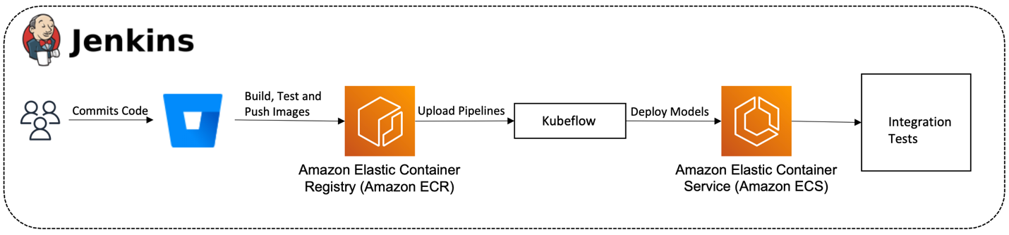
CI/CD Deployment workflow. This diagram describes the Data Science build and deployment workflow. The CI/CD process is driven by Jenkins.
Security
In consolidating our data science workflows, we were able to centralize our approach to securing the training pipeline. In this section, we discuss our approach to data and cluster security.
Data security
Data security is of the utmost importance at athenahealth. For this reason, we develop and maintain infrastructure that is fully compliant with the regulations and standards that protect the security and integrity of these data.
To ensure we meet data compliance standards, we provision our AWS infrastructure in accordance with our athenahealth enterprise guidelines. The two main stores for data are Amazon RDS for highly scalable pipeline metadata and Amazon S3 for pipeline and model artifacts. For Amazon S3, we ensure the buckets are encrypted, HTTPS endpoints are enforced, and the bucket policies and AWS Identity and Access Management (IAM) roles follow the principles of least privilege when permitting access to the data. This is true for Amazon RDS data as well: encryption is always enabled, and the security groups and credential access follow the principle of least privilege. This standardization ensures that only authorized parties have access to the data, and this access is tracked.
In addition to these measures, the platform also undergoes security threat assessments and continuous security and compliance scans.
We also address data retention requirements via data lifecycle management for all S3 buckets that contain sensitive data. This policy automatically moves data to Amazon S3 Glacier after 30 days of creation. Exceptions to this are managed through data retrieval requests and are approved or denied on a case-by-case basis. This ensures that all workflows comply with the data retention policy. This also solves the problem with recovering data if a model performs poorly, and retraining is required, or when a new model must be evaluated against a historical iteration of an older model’s dataset.
For restricting access to Amazon S3 and Amazon RDS from within Kubeflow on AWS and Amazon EKS, we use IRSA (IAM Roles for Service Accounts), which provides IAM-based permission provisioning for resources within Kubernetes. Each tenant in Kubeflow has a unique pre-created service account which we bind to an IAM role created specifically to fulfill the tenant access requirements. User access to tenants is also restricted using the Amazon Cognito user pools group membership for each user. When a user is authenticated to the cluster, the generated token contains group claims, and Kubernetes RBAC uses this information to allow or deny access to a particular resource in the cluster. This setup is explained in more detail in the next section.
Cluster security using multi-user isolation
As we noted in the previous section, data scientists perform exploratory data analyses, run data analytics, and train ML models. To allocate resources, organize data, and manage workflows based on projects, Kubeflow on AWS provides isolation based on Kubernetes namespaces. This isolation works for interacting with the Kubeflow UI; however, it doesn’t provide any tooling to control access to the Kubernetes API using Kubectl. This means that user access can be controlled on the Kubeflow UI but not over the Kubernetes API via Kubectl.
The architecture described in the following diagram addresses this issue by unifying access to projects in Kubeflow based on group memberships. To achieve this, we took advantage of the Kubeflow on AWS manifests, which have integration with Amazon Cognito user pools. In addition, we use Kubernetes role-based access control (RBAC) to control authorization within the cluster. The user permissions are provisioned based on Amazon Cognito group membership. This information is passed to the cluster with the token generated by the OIDC client. This process is simplified thanks to the built-in Amazon EKS functionality that allows associating OIDC identity providers to authenticate with the cluster.
By default, Amazon EKS authentication is performed by the IAM authenticator, which is a tool that enables authenticating with an EKS cluster using IAM credentials. This authentication method has its merits; however, it’s not suitable for our use case because athenahealth uses Microsoft Azure Active Directory for identity service across the organization.
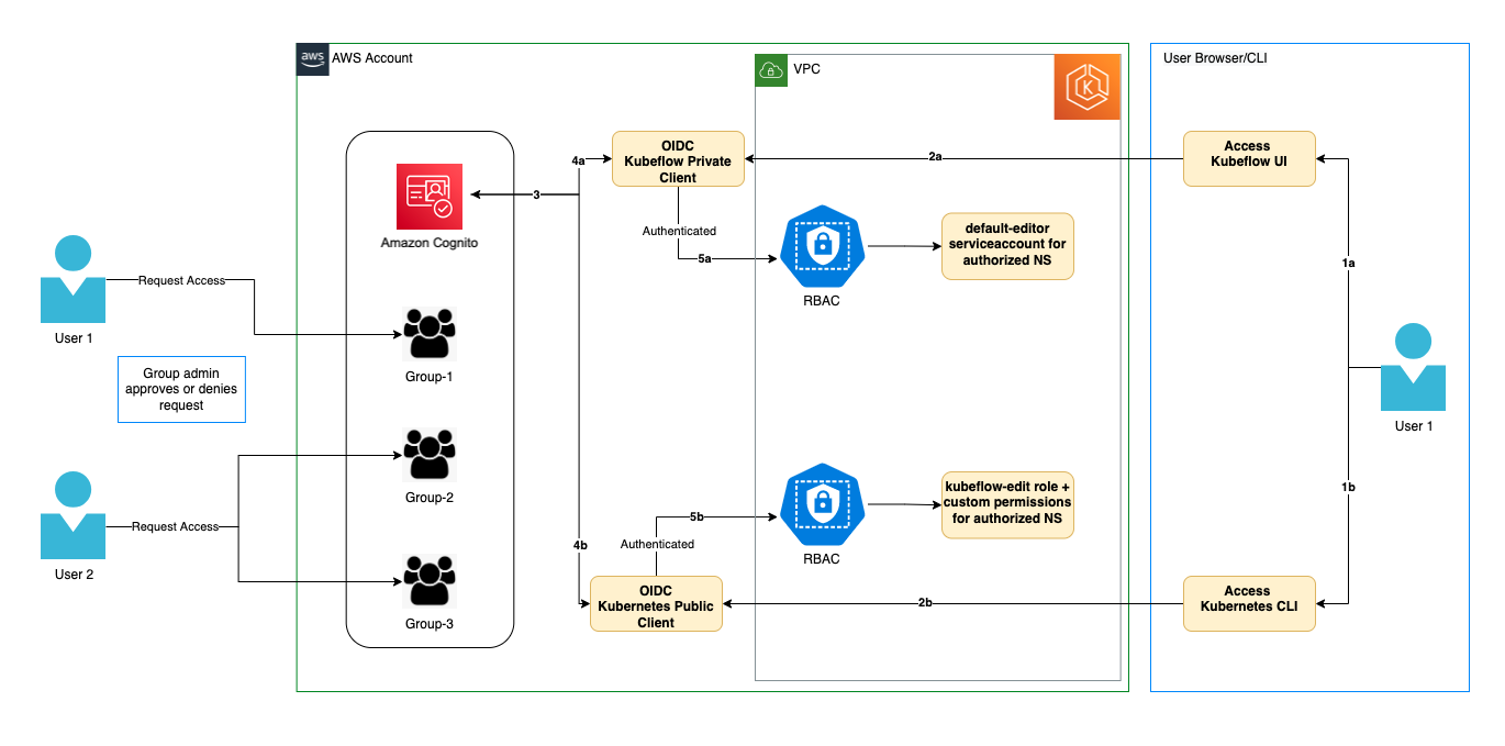
Kubernetes namespace isolation. Data Scientists can obtain membership to a single or multiple groups as needed for their work. Access is reviewed on a regular basis and removed as appropriate.
Azure Active Directory, being an enterprise-wide identity service, is the source of truth for controlling user access to the Kubeflow cluster. The setup for this includes creating an Azure Enterprise Application that acts as service principal and adding groups for various tenants that require access to the cluster. This setup on Azure is mirrored in Amazon Cognito by setting up a federated OIDC identity provider that outsources authentication responsibility to Azure. The access to Azure groups is controlled by SailPoint IdentityIQ, which sends access requests to the project owner to allow or deny as appropriate. In the Amazon Cognito user pool, two application clients are created: one is used to set up the authentication for the Kubernetes cluster using the OIDC identity provider, and the other to secure Kubeflow authentication into the Kubeflow UI. These clients are configured to pass group claims upon authentication with the cluster, and these group claims are used alongside RBAC to set up authorization within the cluster.
Kubernetes RBAC role bindings are set up between groups and the cluster role Kubeflow-edit, which is created upon installing Kubeflow in the cluster. This role binding ensures any user interacting with the cluster after logging in via OIDC can access the namespaces they have permissions for as defined in their group claims. Although this works for users interacting with the cluster using Kubectl, the Kubeflow UI currently doesn’t provision access to users based on group membership because it doesn’t use RBAC. Instead, it uses the Istio Authorization Policy resource to control access for users. To overcome this challenge, we developed a custom controller that synchronizes users by polling Amazon Cognito groups and adds or removes corresponding role bindings for each user rather than by group. This setup enables users to have the same level of permissions when interacting with both the Kubeflow UI and Kubectl.
Operational efficiency
In this section, we discuss how we took advantage of the open source and AWS tools available to us to manage and debug our workflows as well as to minimize the operational impact of upgrading Kubeflow.
Logging and monitoring
For logging, we utilize FluentD to push all our container logs to Amazon OpenSearch Service and system metrics to Prometheus. We then use Kibana and the Grafana UI for searching and filtering logs and metrics. The following diagram describes how we set this up.
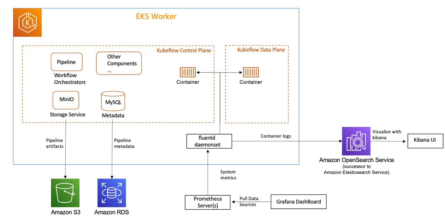
Kubeflow Logging. We use both Grafana UI and Kibana to view and sift through the logs
The following screenshot is a Kibana UI view from our pipeline.
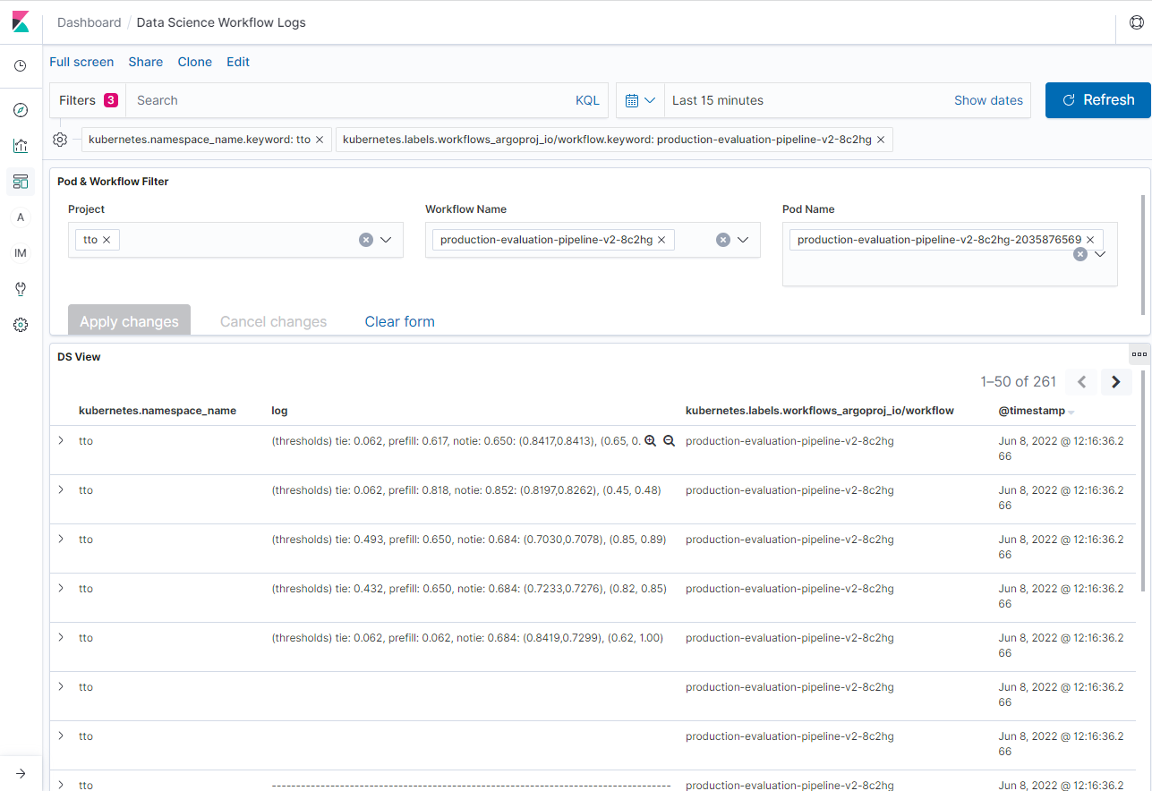
Sample Kibana UI View. Kibana allows for customized views.
Safe Kubeflow cluster upgrades
As we onboard users to Kubeflow on AWS, we maintain a reliable and consistent user experience while allowing the MLOps team to stay agile with releasing and integrating new features. On the surface, Kustomize seems modular for us to enable working and upgrading one component at a time without impacting others, thereby allowing us to add new capabilities with minimal disruption to the users. However, in practice there are scenarios where the best approach is to simply spin up a new Kubernetes cluster rather than applying component-level upgrades for existing clusters. We found two use cases where it made more sense to create completely new clusters:
- Upgrading to a Kubernetes version where AWS does provide in-place cluster upgrades. However, it becomes difficult to test if each of the Kubeflow and Kubernetes resources are working as intended and the manifests retain backward compatibility.
- Upgrading Kubeflow to a newer release where there are several features added or modified and it almost always is not a promising idea to perform in-place upgrades on an existing Kubernetes cluster.
In addressing this issue, we developed a strategy that enables us to have safe cluster replacements without impacting any existing workloads. To achieve this, we had to meet the following criteria:
- Separate the Kubeflow storage and compute resources so that the pipeline metadata, pipeline artifacts, and user data are retained when deprovisioning the older cluster
- Integrate with Kubeflow on AWS manifests so that when a Kubeflow version upgrade occurs, minimal changes are required
- Have an effortless way to roll back if things go wrong after cluster upgrade
- Have a simple interface to promote a candidate cluster to production
The following diagram illustrates this architecture.
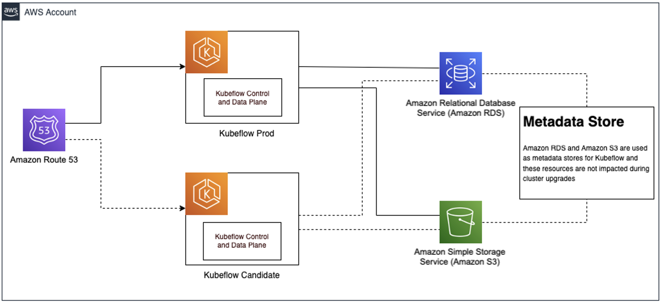
Safe Kubeflow Cluster Upgrade. Once testing of the Kubeflow Candidate is successful, it is promoted to Kubeflow Prod through an update to Route 53.
Kubeflow on AWS manifests come pre-packaged with Amazon RDS and Amazon S3 integrations. With these managed services acting as common data stores, we can set up a blue-green deployment strategy. To achieve this, we ensured that the pipeline metadata is persisted in Amazon RDS, which works independently of the EKS cluster, and the pipeline logs and artifacts are persisted in Amazon S3. In addition to pipeline metadata and artifacts, we also set up FluentD to route pod logs to Amazon OpenSearch Service.
This ensures that the storage layer is completely separated from the compute layer and thereby enables testing changes during Kubeflow version updates on a completely new EKS cluster. After all the tests are successful, we’re able to simply change the Amazon Route 53 DNS record to the candidate cluster hosting Kubeflow. Also, we keep the old cluster running as backup for a few days just in case we need to roll back.
Benefits of Amazon EKS and Kubeflow on AWS for our ML pipeline
Amazon EKS and the Kubeflow on AWS package moved our development workflow to a pattern that strongly encourages repeatable model training. These tools allow us to have fully defined clusters with fully defined tenants and run fully defined code.
A lot of wins from building this platform are less quantitative and have more to do with how the workflows have improved for both platform developers and users. For example, MinIO was replaced with direct access to Amazon S3, which moves us closer to our original workflows and reduces the number of services we must maintain. We are also able to utilize Amazon RDS as the backend for Kubeflow, which enables easier migrations between clusters and gives us the ability to back up our pipelines nightly.
We also found the improvements in the Kubeflow integration with AWS managed services beneficial. For example, with Amazon RDS, Amazon S3, and Amazon Cognito preconfigured in the Kubeflow on AWS manifests, we save time and effort updating to newer distributions of Kubeflow. When we used to modify the official Kubeflow manifests manually, updating to a new version would take several weeks, from design to testing.
Switching to Amazon EKS gives us the opportunity to define our cluster in Kustomize (now part of Kubectl) and Terraform. It turns out that for platform work, Kubernetes and Terraform are very easy to work with after putting in enough time to learn. After many iterations, the tools available to us make it very easy to perform standard platform operations like upgrading a component or swapping out an entire development cluster. Compared to running jobs off raw Amazon Elastic Compute Cloud (Amazon EC2) instances, it’s hard to compare what an enormous difference it makes to have well-defined pods with guaranteed resource cleanup and retry mechanisms built in.
Kubernetes provides great security standards, and we have only scratched the surface of what the multi-user isolation allows us to do. We see multi-user isolation as a pattern that has more payoff in the future when the training platform produces production-level data, and we bring on developers from outside our team.
Meanwhile, Kubeflow allows us to have reproducible model training. Even with the same data, no training produces identical models, but we have the next best thing. With Kubeflow, we know exactly what code and data were used to train a model. Onboarding has greatly improved because each step in our pipeline is clearly and programmatically defined. When new data scientists have the task of fixing a bug, they need much less handholding because there is a clear structure to how outputs of code are used between stages.
Using Kubeflow also yields a lot of performance improvements compared to running on a single EC2 instance. Often in model training, data scientists need different tools and optimizations for preprocessing and training. For example, preprocessing is often run using distributed data processing tools, like Spark, whereas training is often run using GPU instances. With Kubeflow pipelines, they can specify different instance types for different stages in the pipeline. This allows them to use the powerful GPU instances in one stage and a fleet of smaller machines for distributed processing in another stage. Also, because Kubeflow pipelines describe the dependencies between stages, the pipelines can run stages in parallel.
Finally, because we created a process for adding tenants to the cluster, there is now a more formal way to register teams to a tenant on the cluster. Because we use Kubecost to track costs in our EKS cluster, it allows us to attribute cost to a single project rather than having cost attributed at the account level, which includes all data science projects. Kubecost presents a report of the money spent per namespace, which is tightly coupled to the tenant or team that is responsible for running the pipeline.
Despite all the benefits, we would caution to only undertake this kind of migration if there is total buy-in from users. Users that put in the time get a lot of benefits from using Amazon EKS and Kubernetes, but there is a significant learning curve.
Conclusion
With the implementation of the Kubeflow on AWS pipeline in our end-to-end ML infrastructure, we were able to consolidate and standardize our data science workflows while retaining our essential tooling (such as CI/CD and model serving). Our data scientists can now move between projects based on this workflow without the overhead of learning how to maintain a completely different toolset. For some of our models, we were also pleasantly surprised at the speed of the new workflow (five times faster), which allowed for more training iterations and consequently producing models with better predictions.
We also have established a solid foundation to augment our MLOps capabilities and scale the number and size of our projects. For example, as we harden our governance posture in model lineage and tracking, we have reduced our focus from over 15 workflows to just one. And when the Log4shell vulnerability came to light in late 2021, we were able to focus on a single workflow and quickly remediate as needed (performing Amazon Elastic Container Registry (Amazon ECR) scans, upgrading Amazon OpenSearch Service, updating our tooling, and more) with minimal impact to the ongoing work by the data scientists. As AWS and Kubeflow enhancements become available, we can incorporate them as we see fit.
This brings us to an important and understated aspect of our Kubeflow on AWS adoption. One of the critical outcomes of this journey is the ability to roll out upgrades and enhancements to Kubeflow seamlessly for our data scientists. Although we discussed our approach to this earlier, we also rely on the Kubeflow manifests provided by AWS. We started our Kubeflow journey as a proof of concept in 2019, prior to the release of version 1.0.0. (We’re currently on 1.4.1, evaluating 1.5. AWS is already working on the 1.6 version.) In the intervening 3 years, there have been at least six releases with substantial content. Through their disciplined approach to integrating and validating these upgrades and releasing the manifests on a predictable, reliable schedule, the Kubeflow team at AWS has been crucial in enabling the athenahealth MLOps team to plan our development roadmap, and consequently our resource allocations and areas of focus, further into the future with greater confidence.
You can follow the AWS Labs GitHub repository to track all AWS contributions to Kubeflow. You can also find AWS teams on the Kubeflow #AWS Slack Channel; your feedback there helps AWS prioritize the next features to contribute to the Kubeflow project.
About the authors
 Kanwaljit Khurmi is a Senior Solutions Architect at Amazon Web Services. He works with the AWS customers to provide guidance and technical assistance helping them improve the value of their solutions when using AWS. Kanwaljit specializes in helping customers with containerized and machine learning applications.
 Tyler Kalbach is a Principal Member of Technical Staff at athenahealth. Tyler has approximately 7 years of experience in Analytics, Data Science, Neural Networks, and development of Machine Learning applications in the Healthcare space. He has contributed to several Machine Learning solutions that are currently serving production traffic. Currently working as a Principal Data Scientist in athenahealth’s Engineering organization, Tyler has been part of the team that has built the new Machine Learning Training Platform for athenahealth from the inception of that effort.
 Victor Krylov is a Principal Member of Technical Staff at athenahealth. Victor is an engineer and scrum master, helping data scientists build secure fast machine learning pipelines. In athenahealth he has worked on interfaces, clinical ordering, prescriptions, scheduling, analytics and now machine learning. He values cleanly written and well unit tested code, but has an unhealthy obsession with code one-liners. In his spare time he enjoys listening to podcasts while walking his dog.
 Sasank Vemuri is a Lead Member of Technical Staff at athenahealth. He has experience working with developing data driven solutions across domains such as healthcare, insurance and bioinformatics. Sasank currently works with designing and developing machine learning training and inference platforms on AWS and Kubernetes that help with training and deploying ML solutions at scale.
 Anu Tumkur is an Architect at athenahealth. Anu has over two decades of architecture, design, development experience building various software products in machine learning, cloud operations, big data, real-time distributed data pipelines, ad tech, data analytics, social media analytics. Anu currently works as an architect in athenahealth’s Product Engineering organization on the Machine Learning Platform and Data Pipeline teams.
 William Tsen is a Senior Engineering Manager at athenahealth. He has over 20 years of engineering leadership experience building solutions in healthcare IT, big data distributed computing, intelligent optical networks, real-time video editing systems, enterprise software, and group healthcare underwriting. William currently leads two awesome teams at athenahealth, the Machine Learning Operations and DevOps engineering teams, in the Product Engineering organization.
Read More
 Jeremy Singh is a Partner Marketing Manager for storage partners within the AWS Partner Network. In his spare time, he enjoys traveling, going to the beach, and spending time with his dog Bolin.


 Frank Liu is a Software Engineer for AWS Deep Learning. He focuses on building innovative deep learning tools for software engineers and scientists. In his spare time, he enjoys hiking with friends and family.
 Qingwei Li is a Machine Learning Specialist at Amazon Web Services. He received his Ph.D. in Operations Research after he broke his advisor’s research grant account and failed to deliver the Nobel Prize he promised. Currently he helps customers in the financial service and insurance industry build machine learning solutions on AWS. In his spare time, he likes reading and teaching.