Organizations across industries such as healthcare, finance and lending, legal, retail, and manufacturing often have to deal with a lot of documents in their day-to-day business processes. These documents contain critical information that are key to making decisions on time in order to maintain the highest levels of customer satisfaction, faster customer onboarding, and lower customer churn. In most cases, documents are processed manually to extract information and insights, which is time-consuming, error-prone, expensive, and difficult to scale. There is limited automation available today to process and extract information from these documents. Intelligent document processing (IDP) with AWS artificial intelligence (AI) services helps automate information extraction from documents of different types and formats, quickly and with high accuracy, without the need for machine learning (ML) skills. Faster information extraction with high accuracy helps in making quality business decisions on time, while reducing overall costs.
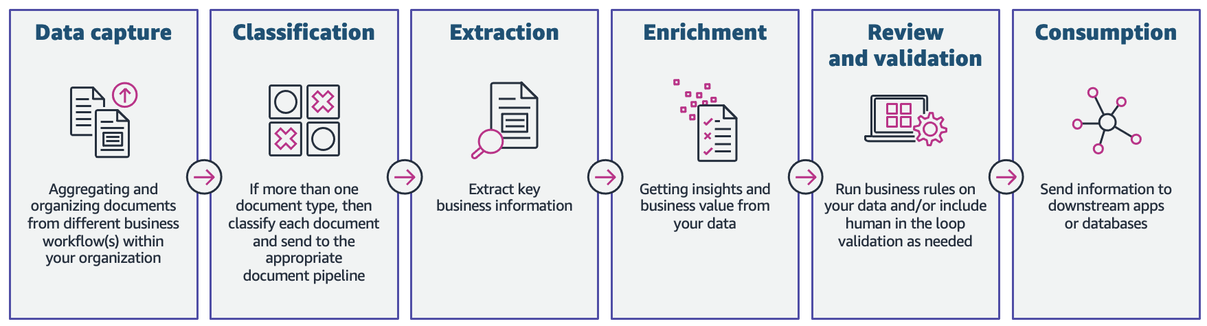
Although the stages in an IDP workflow may vary and be influenced by use case and business requirements, the following figure shows the stages that are typically part of an IDP workflow. Processing documents such as tax forms, claims, medical notes, new customer forms, invoices, legal contracts, and more are just a few of the use cases for IDP.
In this two-part series, we discuss how you can automate and intelligently process documents at scale using AWS AI services. In this post, we discuss the first three phases of the IDP workflow. In part 2, we discuss the remaining workflow phases.
Solution overview
The following architecture diagram shows the stages of an IDP workflow. It starts with a data capture stage to securely store and aggregate different file formats (PDF, JPEG, PNG, TIFF) and layouts of documents. The next stage is classification, where you categorize your documents (such as contracts, claim forms, invoices, or receipts), followed by document extraction. In the extraction stage, you can extract meaningful business information from your documents. This extracted data is often used to gather insights via data analysis, or sent to downstream systems such as databases or transactional systems. The following stage is enrichment, where documents can be enriched by redacting protected health information (PHI) or personally identifiable information (PII) data, custom business term extraction, and so on. Finally, in the review and validation stage, you can include a human workforce for document reviews to ensure the outcome is accurate.
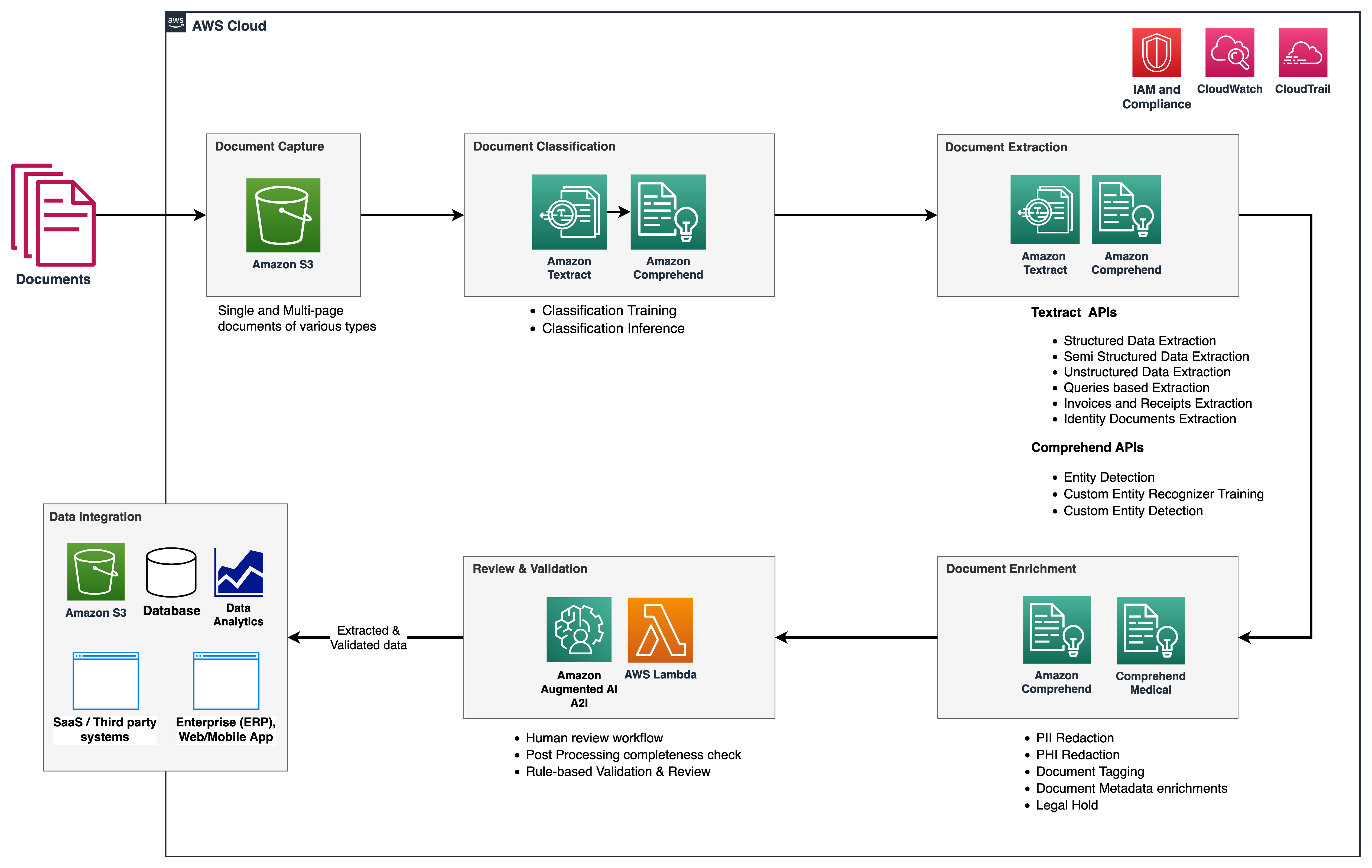
For the purposes of this post, we consider a set of sample documents such as bank statements, invoices, and store receipts. The document samples, along with sample code, can be found in our GitHub repository. In the following sections, we walk you through these code samples along with real practical application. We demonstrate how you can utilize ML capabilities with Amazon Textract, Amazon Comprehend, and Amazon Augmented AI (Amazon A2I) to process documents and validate the data extracted from them.
Amazon Textract is an ML service that automatically extracts text, handwriting, and data from scanned documents. It goes beyond simple optical character recognition (OCR) to identify, understand, and extract data from forms and tables. Amazon Textract uses ML to read and process any type of document, accurately extracting text, handwriting, tables, and other data with no manual effort.
Amazon Comprehend is a natural-language processing (NLP) service that uses ML to extract insights about the content of the documents. Amazon Comprehend can identify critical elements in documents, including references to language, people, and places, and classify them into relevant topics or clusters. It can perform sentiment analysis to determine the sentiment of a document in real time using single document or batch detection. For example, it can analyze the comments on a blog post to know if your readers like the post or not. Amazon Comprehend also detects PII like addresses, bank account numbers, and phone numbers in text documents in real time and asynchronous batch jobs. It can also redact PII entities in asynchronous batch jobs.
Amazon A2I is an ML service that makes it easy to build the workflows required for human review. Amazon A2I brings human review to all developers, removing the undifferentiated heavy lifting associated with building human review systems or managing large numbers of human reviewers, whether it runs on AWS or not. Amazon A2I integrates both with Amazon Textract and Amazon Comprehend to provide you the ability to introduce human review steps within your intelligent document processing workflow.
Data capture phase
You can store documents in a highly scalable and durable storage like Amazon Simple Storage Service (Amazon S3). Amazon S3 is an object storage service that offers industry-leading scalability, data availability, security, and performance. Amazon S3 is designed for 11 9’s of durability and stores data for millions of customers all around the world. Documents can come in various formats and layouts, and can come from different channels like web portals or email attachments.
Classification phase
In the previous step, we collected documents of various types and formats. In this step, we need to categorize the documents before we can do further extraction. For that, we use Amazon Comprehend custom classification. Document classification is a two-step process. First, you train an Amazon Comprehend custom classifier to recognize the classes that are of interest to you. Next, you deploy the model with a custom classifier real-time endpoint and send unlabeled documents to the real-time endpoint to be classified.
The following figure represents a typical document classification workflow.

To train the classifier, identify the classes you’re interested in and provide sample documents for each of the classes as training material. Based on the options you indicated, Amazon Comprehend creates a custom ML model that it trains based on the documents you provided. This custom model (the classifier) examines each document you submit. It returns either the specific class that best represents the content (if you’re using multi-class mode) or the set of classes that apply to it (if you’re using multi-label mode).
Prepare training data
The first step is to extract text from documents required for the Amazon Comprehend custom classifier. To extract the raw text information for all the documents in Amazon S3, we use the Amazon Textract detect_document_text() API. We also label the data according to the document type to be used to train a custom Amazon Comprehend classifier.
The following code has been trimmed down for simplification purposes. For the full code, refer to the GitHub sample code for textract_extract_text(). The function call_textract() is a wr4apper function that calls the AnalyzeDocument API internally, and the parameters passed to the method abstract some of the configurations that the API needs to run the extraction task.
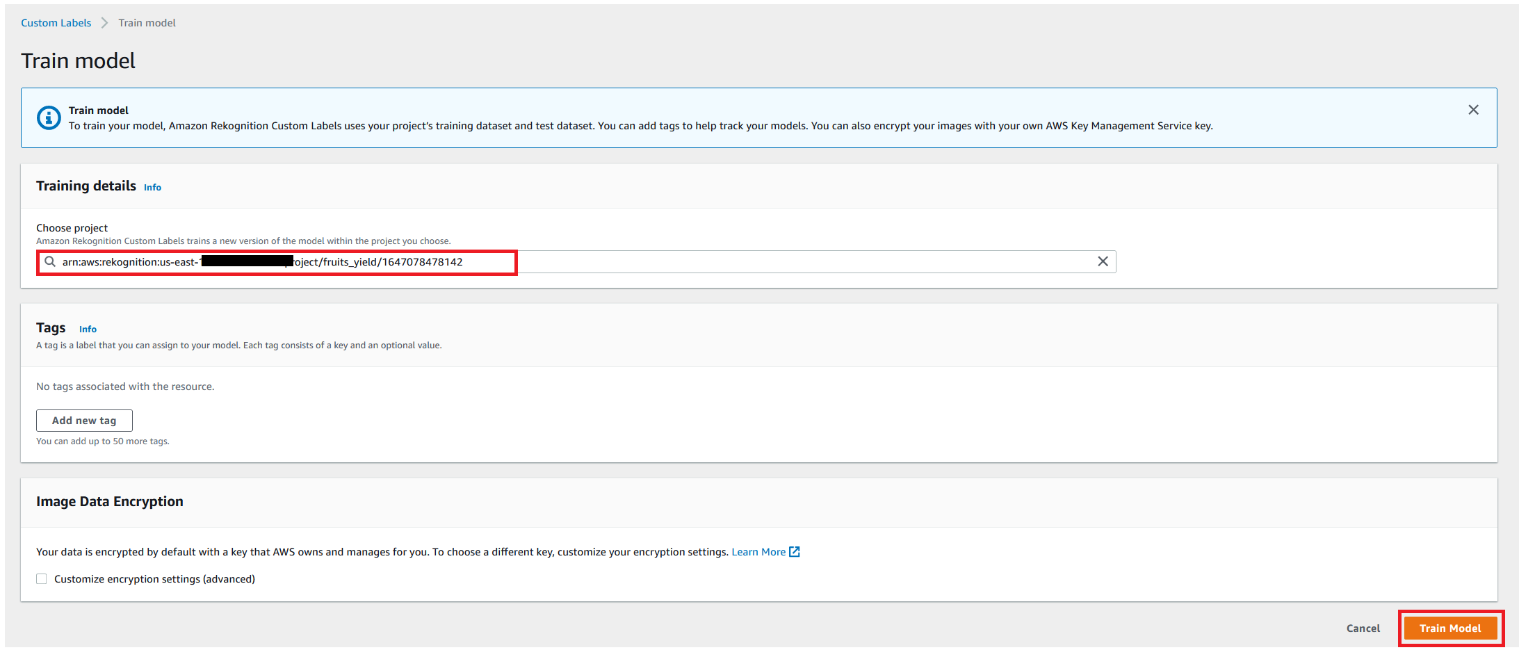
Train a custom classifier
In this step, we use Amazon Comprehend custom classification to train our model for classifying the documents. We use the CreateDocumentClassifier API to create a classifier that trains a custom model using our labeled data. See the following code:
Deploy a real-time endpoint
To use the Amazon Comprehend custom classifier, we create a real-time endpoint using the CreateEndpoint API:
Classify documents with the real-time endpoint
After the Amazon Comprehend endpoint is created, we can use the real-time endpoint to classify documents. We use the comprehend.classify_document() function with the extracted document text and inference endpoint as input parameters:

We recommend going through the detailed document classification sample code on GitHub.
Extraction phase
Amazon Textract lets you extract text and structured data information using the Amazon Textract DetectDocumentText and AnalyzeDocument APIs, respectively. These APIs respond with JSON data, which contains WORDS, LINES, FORMS, TABLES, geometry or bounding box information, relationships, and so on. Both DetectDocumentText and AnalyzeDocument are synchronous operations. To analyze documents asynchronously, use StartDocumentTextDetection.
Structured data extraction
You can extract structured data such as tables from documents while preserving the data structure and relationships between detected items. You can use the AnalyzeDocument API with the FeatureType as TABLE to detect all tables in a document. The following figure illustrates this process.

See the following code:
We run the analyze_document() method with the FeatureType as TABLES on the employee history document and obtain the table extraction in the following results.

Semi-structured data extraction
You can extract semi-structured data such as forms or key-value pairs from documents while preserving the data structure and relationships between detected items. You can use the AnalyzeDocument API with the FeatureType as FORMS to detect all forms in a document. The following diagram illustrates this process.

See the following code:
Here, we run the analyze_document() method with the FeatureType as FORMS on the employee application document and obtain the table extraction in the results.

Unstructured data extraction
Amazon Textract is optimal for dense text extraction with industry-leading OCR accuracy. You can use the DetectDocumentText API to detect lines of text and the words that make up a line of text, as illustrated in the following figure.

See the following code:
Now we run the detect_document_text() method on the sample image and obtain raw text extraction in the results.

Invoices and receipts
Amazon Textract provides specialized support to process invoices and receipts at scale. The AnalyzeExpense API can extract explicitly labeled data, implied data, and line items from an itemized list of goods or services from almost any invoice or receipt without any templates or configuration. The following figure illustrates this process.

See the following code:
Amazon Textract can find the vendor name on a receipt even if it’s only indicated within a logo on the page without an explicit label called “vendor”. It can also find and extract expense items, quantity, and prices that aren’t labeled with column headers for line items.

Identity documents
The Amazon Textract AnalyzeID API can help you automatically extract information from identification documents, such as driver’s licenses and passports, without the need for templates or configuration. We can extract specific information, such as date of expiry and date of birth, as well as intelligently identify and extract implied information, such as name and address. The following diagram illustrates this process.

See the following code:
We can use tabulate to get a pretty printed output:

We recommend going through the detailed document extraction sample code on GitHub. For more information about the full code samples in this post, refer to the GitHub repo.
Conclusion
In this first post of a two-part series, we discussed the various stages of IDP and a solution architecture. We also discussed document classification using an Amazon Comprehend custom classifier. Next, we explored the ways you can use Amazon Textract to extract information from unstructured, semi-structured, structured, and specialized document types.
In part 2 of this series, we continue the discussion with the extract and queries features of Amazon Textract. We look at how to use Amazon Comprehend pre-defined entities and custom entities to extract key business terms from documents with dense text, and how to integrate an Amazon A2I human-in-the-loop review in your IDP processes.
We recommend reviewing the security sections of the Amazon Textract, Amazon Comprehend, and Amazon A2I documentation and following the guidelines provided. Also, take a moment to review and understand the pricing for Amazon Textract, Amazon Comprehend, and Amazon A2I.
About the authors
 Suprakash Dutta is a Solutions Architect at Amazon Web Services. He focuses on digital transformation strategy, application modernization and migration, data analytics, and machine learning.
 Sonali Sahu is leading Intelligent Document Processing AI/ML Solutions Architect team at Amazon Web Services. She is a passionate technophile and enjoys working with customers to solve complex problems using innovation. Her core area of focus is artificial intelligence and machine learning for intelligent document processing.
 Anjan Biswas is a Senior AI Services Solutions Architect with a focus on AI/ML and data analytics. Anjan is part of the world-wide AI services team and works with customers to help them understand and develop solutions to business problems with AI and ML. Anjan has over 14 years of experience working with global supply chain, manufacturing, and retail organizations, and is actively helping customers get started and scale on AWS AI services.
 Chinmayee Rane is an AI/ML Specialist Solutions Architect at Amazon Web Services. She is passionate about applied mathematics and machine learning. She focuses on designing intelligent document processing solutions for AWS customers. Outside of work, she enjoys salsa and bachata dancing.


 Jian Zhang is an applied scientist who has been using machine learning techniques to help customers solve various problems, such as fraud detection, decoration image generation, and more. He has successfully developed graph-based machine learning, particularly graph neural network, solutions for customers in China, USA, and Singapore. As an enlightener of AWS’s graph capabilities, Zhang has given many public presentations about the GNN, the Deep Graph Library (DGL), Amazon Neptune, and other AWS services.
 Mengxin Zhu is a manager of Solutions Architects at AWS, with a focus on designing and developing reusable AWS solutions. He has been engaged in software development for many years and has been responsible for several startup teams of various sizes. He also is an advocate of open-source software and was an Eclipse Committer.
 Haozhu Wang is a research scientist at Amazon ML Solutions Lab, where he co-leads the Reinforcement Learning Vertical. He helps customers build advanced machine learning solutions with the latest research on graph learning, natural language processing, reinforcement learning, and AutoML. Haozhu received his PhD in Electrical and Computer Engineering from the University of Michigan.