Posts in category: Amazon AWS

In the end, it came down to 213 thousandths of a second! That was the difference between the two best times in the finale of the first AWS AWS DeepRacer Student Wildcard event hosted in Ottawa, Canada this May.

I watched in awe as 13 students competed in a live wildcard race for the AWS DeepRacer Student League, the first global autonomous racing league for students offering educational material and resources to get hands on and start with machine learning (ML).

Students hit the starting line to put their ML skills to the test in Canada’s capital where members of parliament cheered them on, including Parliamentary Secretary for Innovation, Science and Economic Development, Andy Fillmore. Daphne Hong, a fourth-year engineering student at the University of Calgary, won the race with a lap time of 11:167 seconds. Not far behind were Nixon Chan from University of Waterloo and Vijayraj Kharod from Toronto Metropolitan University.

Daphne was victorious after battling nerves earlier in the day when she took practice runs as she struggled turning the corners and quickly adjusted her model. “After seeing how the physical track did compared to the virtual one throughout the day, I was able to make some adjustments and overcome those corners and round them as I intended, so I’m super, super happy about that,” said a beaming Daphne after being presented with her championship trophy.

Daphne also received a $1,000 Amazon Canada Gift Card, while the second and third place racers — Nixon Chan and Vijayraj Kharod — got trophies and $500 gift cards. The top two contestants now have a chance to race virtually in the AWS DeepRacer Student League finale in October. “The whole experience feels like a win for me,” said DeepRacer participant Connor Hunszinger from the University of Alberta.

The event not only highlighted the importance of machine learning education to Canadian policymakers, but also made clear that these young Canadians could be poised to do great things with their ML skills.

The road to the Ottawa Wildcard

This Ottawa race is one of several wildcard events taking place around the world this year as part of the AWS DeepRacer Student League to bring students together to compete live in person. The top two finalists in each Wildcard race will have the opportunity to compete in the AWS DeepRacer Student League finale, with a chance of winning up to $5,000 USD towards their tuition. The top three racers from the student league finale in October will advance to the global AWS DeepRacer League Championship held at AWS re:Invent in Las Vegas this December.

Students who raced in Ottawa began their journey this March when they competed in the global AWS DeepRacer Student League by submitting their model to the virtual 3D simulation environment and posting times to the leaderboard. From the student league, the top student racers across Canada were selected to compete in the wildcard event. Students trained their models in preparation for the event through the virtual environment and then applied their ML models for the first time on a physical track in Ottawa. Each student competitor was given one three-minute attempt to complete their fastest lap with only the speed of the car being controlled.

“Honestly, I don’t really consider my peers here my competitors. I loved being able to work with them. It seems more like a friendly, supportive and collaborative environment. We were always cheering each other on,” says Daphne Hong, AWS DeepRacer Student League Canada Wildcard winner. “This event is great because it allows people who don’t really have that much AI or ML experience to learn more about the industry and see it live with these cars. I want to share my findings and my knowledge with those around me, those in my community and spread the word about ML and AI.”

Building access to machine learning in Canada

Machine learning talent is in hot demand, making up a large portion of AI job postings in Canada. The Canadian economy needs people with the skills recently on display at the DeepRacer event, and Canadian policymakers are intent on building an AI talent pool.

According to the World Economic Forum, 58 million jobs will be created by the growth of machine learning in the next few years, but right now, there are only 300,000 engineers with the relevant training to build and deploy ML models.

That means organizations of all types must not only train their existing workers with ML skills, but also invest in training programs and solutions to develop those capabilities for future workers. AWS is doing its part with a multitude of products for learners of all levels.

• AWS Artificial Intelligence and Machine Learning Scholarship, a $10 million education and scholarship program, aimed at preparing underserved and underrepresented students in tech globally for careers in the space.
• AWS DeepRacer, the world’s first global autonomous racing league, open to developers globally to get started in ML with a 1/18^th scale race car driven by reinforcement learning. Developers can compete in the global racing league for prizes and rewards.
• AWS DeepRacer Student, a version of AWS DeepRacer open to students 16 years and older globally with free access to 20 hours of ML educational content and 10 hours of compute resources for model training monthly at no cost. Participants can compete in the global racing league exclusively for students to win scholarships and prizes.
• Machine Learning University, self service ML training courses with learn at your own pace educational content built by Amazon’s ML scientists.

Cloud computing makes access to machine learning technology a lot easier, faster — and fun, if the AWS DeepRacer Student League Wildcard event was any indication. The race was created by AWS, as an enjoyable, hands-on way to make ML more widely accessible to anyone interested in the technology.

Get started with your machine learning journey and take part in the AWS DeepRacer Student league today for your chance to wins prizes and glory.

About the author

Nicole Foster is Director of AWS Global AI/ML and Canada Public Policy at Amazon, where she leads the direction and strategy of artificial intelligence public policy for Amazon Web Services (AWS) around the world as well as the company’s public policy efforts in support of the AWS business in Canada. In this role, she focuses on issues related to emerging technology, digital modernization, cloud computing, cyber security, data protection and privacy, government procurement, economic development, skilled immigration, workforce development, and renewable energy policy.

Read More

Logistics and transportation companies track ETA (estimated time of arrival), which is a key metric for their business. Their downstream supply chain activities are planned based on this metric. However, delays often occur, and the ETA might differ from the product’s or shipment’s actual time of arrival (ATA), for instance due to shipping distance or carrier-related or weather-related issues. This impacts the entire supply chain, in many instances reducing productivity and increasing waste and inefficiencies. Predicting the exact day a product arrives to a customer is challenging because it depends on various factors such as order type, carrier, origin, and distance.

Analysts working in the logistics and transportation industry have domain expertise and knowledge of shipping and logistics attributes. However, they need to be able to generate accurate shipment ETA forecasts for efficient business operations. They need an intuitive, easy-to-use, no-code capability to create machine learning (ML) models for predicting shipping ETA forecasts.

To help achieve the agility and effectiveness that business analysts seek, we launched Amazon SageMaker Canvas, a no-code ML solution that helps companies accelerate solutions to business problems quickly and easily. SageMaker Canvas provides business analysts with a visual point-and-click interface that allows you to build models and generate accurate ML predictions on your own—without requiring any ML experience or having to write a single line of code.

In this post, we show how to use SageMaker Canvas to predict shipment ETAs.

Solution overview

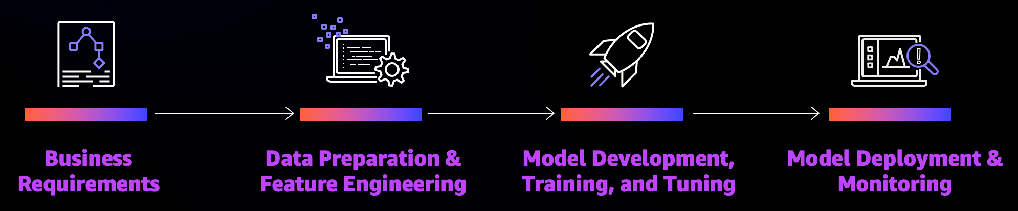
Although ML development is a complex and iterative process, we can generalize an ML workflow into business requirements analysis, data preparation, model development, and model deployment stages.

SageMaker Canvas abstracts the complexities of data preparation and model development, so you can focus on delivering value to your business by drawing insights from your data without a deep knowledge of the data science domain. The following architecture diagram highlights the components in a no-code or low-code solution.

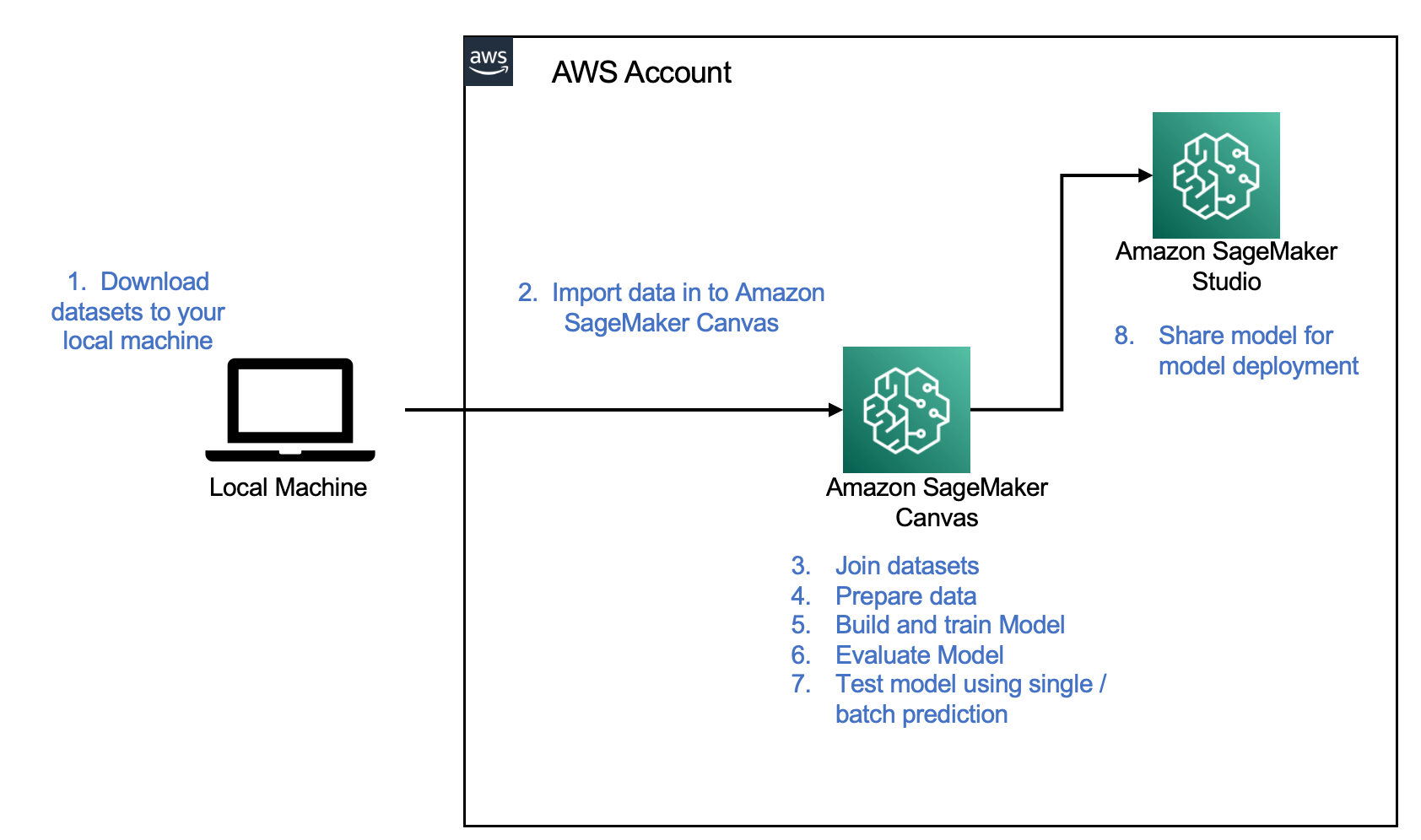
The following are the steps as outlined in the architecture:

1. Download the dataset to your local machine.
2. Import the data into SageMaker Canvas.
3. Join your datasets.
4. Prepare the data.
5. Build and train your model.
6. Evaluate the model.
7. Test the model.
8. Share the model for deployment.

Let’s assume you’re a business analyst assigned to the product shipment tracking team of a large logistics and transportation organization. Your shipment tracking team has asked you to assist in predicting the shipment ETA. They have provided you with a historical dataset that contains characteristics tied to different products and their respective ETA, and want you to predict the ETA for products that will be shipped in the future.

We use SageMaker Canvas to perform the following steps:

1. Import our sample datasets.
2. Join the datasets.
3. Train and build the predictive machine maintenance model.
4. Analyze the model results.
5. Test predictions against the model.

Dataset overview

We use two datasets (shipping logs and product description) in CSV format, which contain shipping log information and certain characteristics of a product, respectively.

The ShippingLogs dataset contains the complete shipping data for all products delivered, including estimated time shipping priority, carrier, and origin. It has approximately 10,000 rows and 12 feature columns. The following table summarizes the data schema.

The ProductDescription dataset contains metadata information of the product that is being shipped in the order. This dataset has approximately 10,000 rows and 5 feature columns. The following table summarizes the data schema.

Prerequisites

An IT administrator with an AWS account with appropriate permissions must complete the following prerequisites:

1. Deploy an Amazon SageMaker domain. For instructions, see Onboard to Amazon SageMaker Domain.
2. Launch SageMaker Canvas. For instructions, see Setting up and managing Amazon SageMaker Canvas (for IT administrators).
3. Configure cross-origin resource sharing (CORS) policies in Amazon Simple Storage Service (Amazon S3) for SageMaker Canvas to enable the upload option from local disk. For instructions, see Give your users the ability to upload local files.

Import the dataset

First, download the datasets (shipping logs and product description) and review the files to make sure all the data is there.

SageMaker Canvas provides several sample datasets in your application to help you get started. To learn more about the SageMaker-provided sample datasets you can experiment with, see Use sample datasets. If you use the sample datasets (canvas-sample-shipping-logs.csv and canvas-sample-product-descriptions.csv) available within SageMaker Canvas, you don’t have to import the shipping logs and product description datasets.

You can import data from different data sources into SageMaker Canvas. If you plan to use your own dataset, follow the steps in Importing data in Amazon SageMaker Canvas.

For this post, we use the full shipping logs and product description datasets that we downloaded.

1. Sign in to the AWS Management Console, using an account with the appropriate permissions to access SageMaker Canvas.
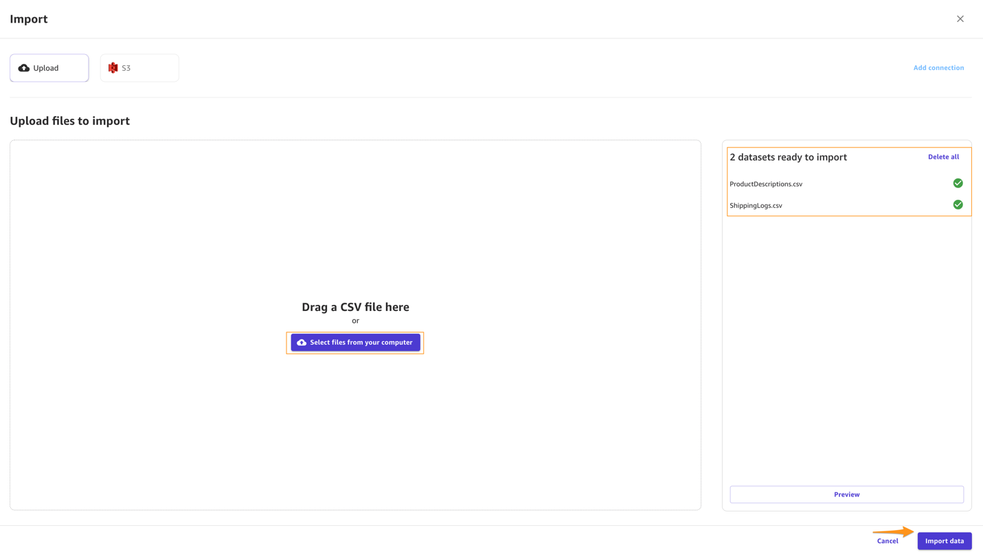
2. On the SageMaker Canvas console, choose Import.
   
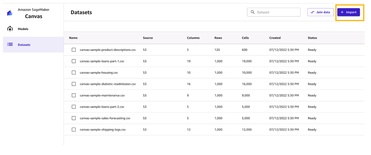
3. Choose Upload and select the files ShippingLogs.csv and ProductDescriptions.csv.
4. Choose Import data to upload the files to SageMaker Canvas.
   

Create a consolidated dataset

Next, let’s join the two datasets.

1. Choose Join data.
   
2. Drag and drop ShippingLogs.csv and ProductDescriptions.csv from the left pane under Datasets to the right pane.
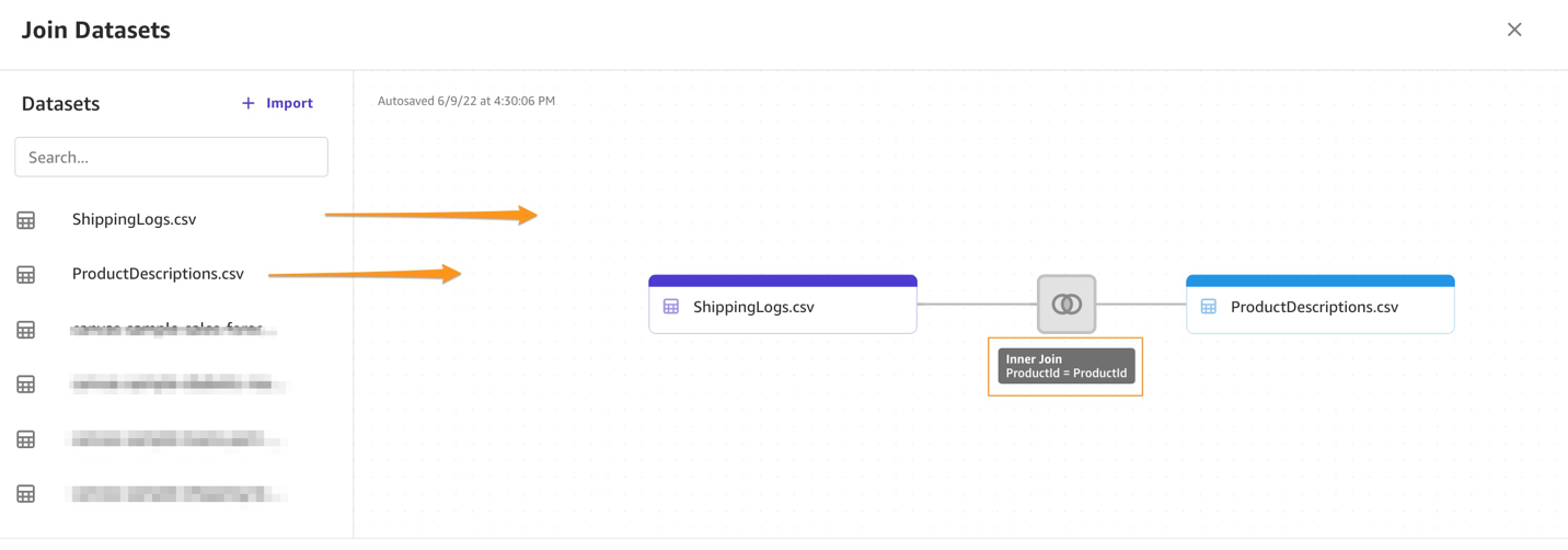
   The two datasets are joined using ProductID as the inner join reference.
3. Choose Import and enter a name for the new joined dataset.
4. Choose Import data.
   

You can choose the new dataset to preview its contents.

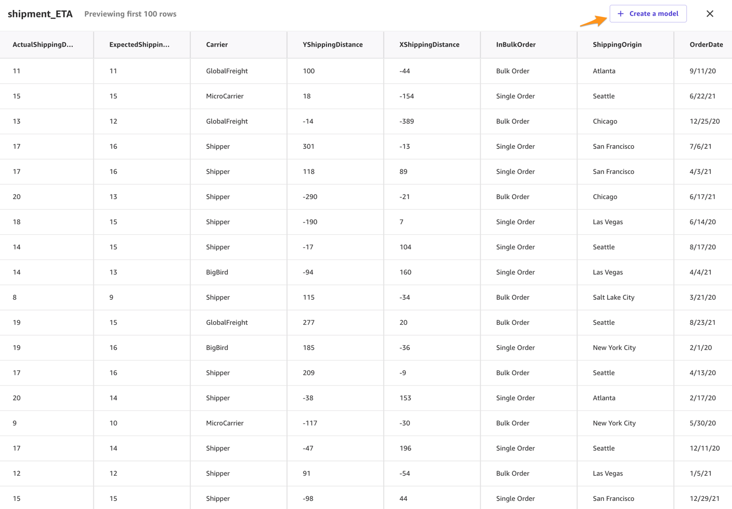
After you review the dataset, you can create your model.

Build and train model

To build and train your model, complete the following steps:

1. For Model name, enter ShippingForecast.
2. Choose Create.
   In the Model view, you can see four tabs, which correspond to the four steps to create a model and use it to generate predictions: Select, Build, Analyze, and Predict.
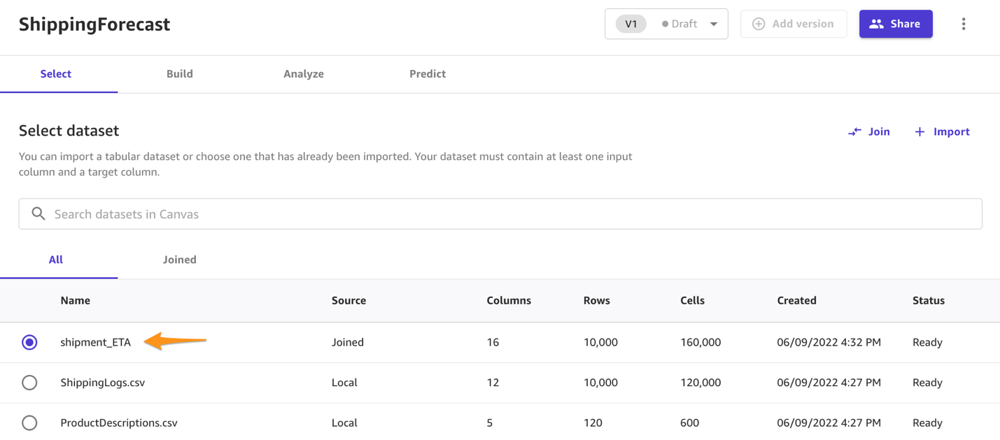
3. On the Select tab, select the ConsolidatedShippingData you created earlier.You can see that this dataset comes from Amazon S3, has 12 columns, and 10,000 rows.
4. Choose Select dataset.
   
   SageMaker Canvas automatically moves to the Build tab.
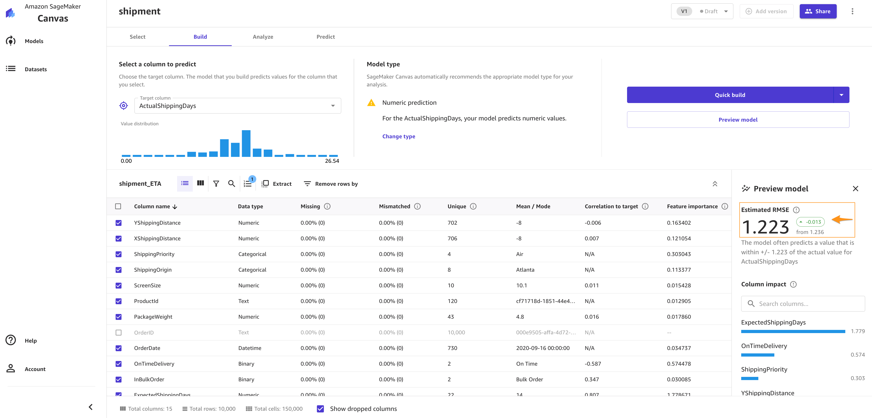
5. On the Build tab, choose the target column, in our case ActualShippingDays.
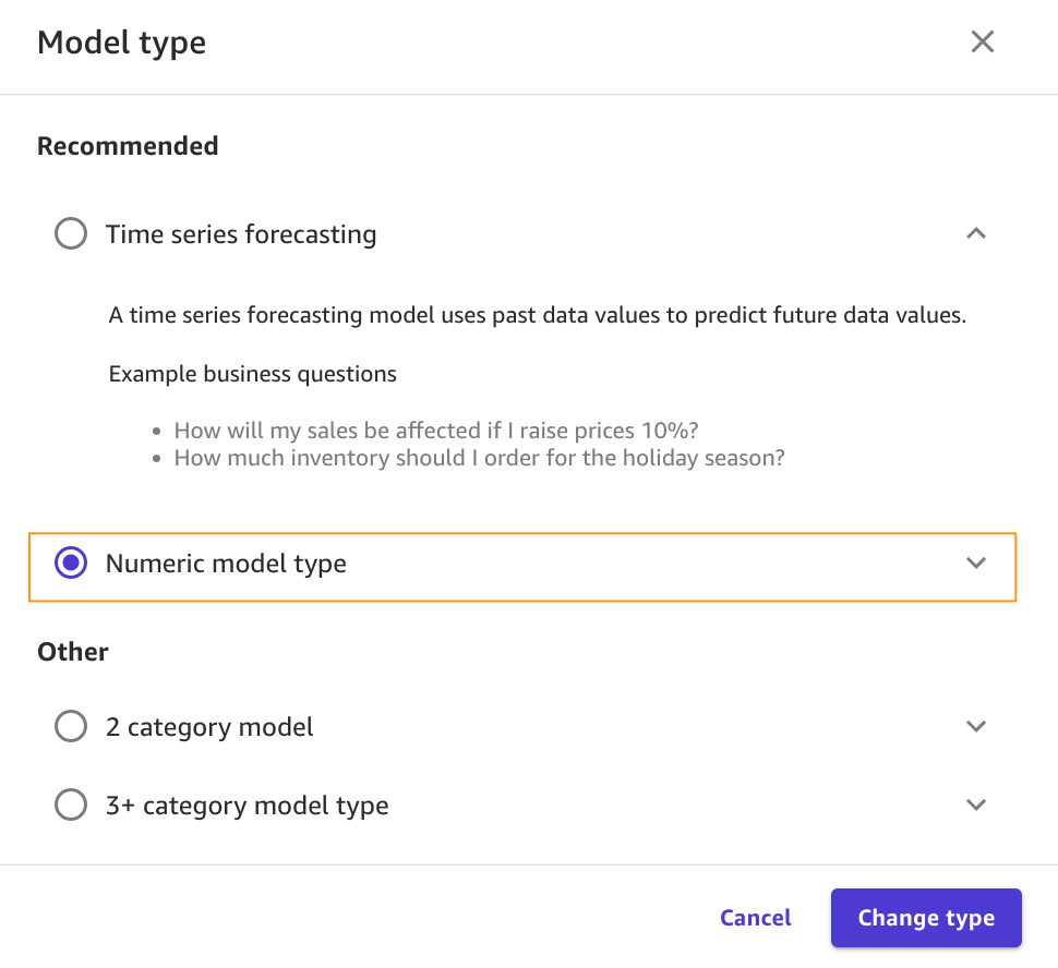
   Because we’re interested in how many days it will take for the goods to arrive for the customer, SageMaker Canvas automatically detects that this is a numeric prediction problem (also known as regression). Regression estimates the values of a dependent target variable based on one or more other variables or attributes that are correlated with it.Because we also have a column with time series data (OrderDate), SageMaker Canvas may interpret this as a time series forecast model type.
6. Before advancing, make sure that the model type is indeed Numeric model type; if that’s not the case, you can select it with the Change type option.
   

Data preparation

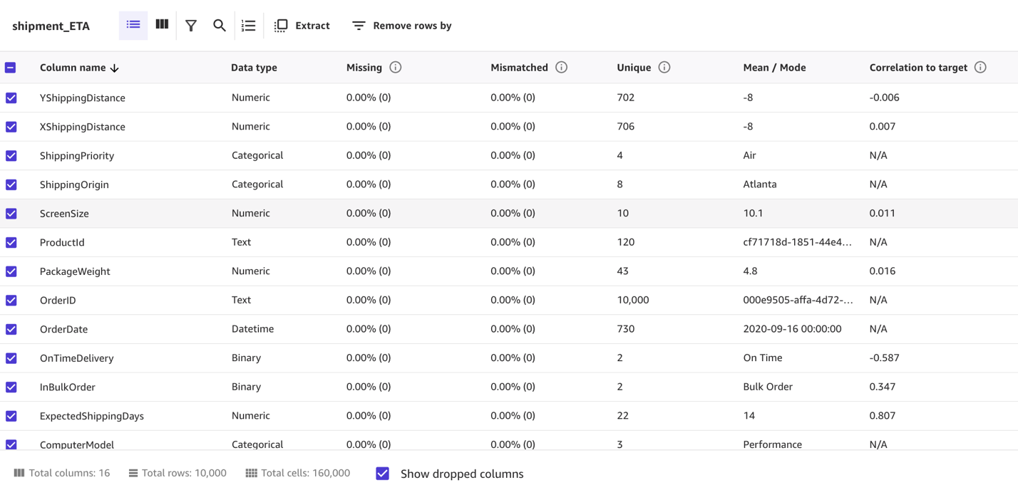
In the bottom half of the page, you can look at some of the statistics of the dataset, including missing and mismatched values, unique values, and mean and median values.

Column view provides you with the listing of all columns, their data types, and their basic statistics, including missing and mismatched values, unique values, and mean and median values. This can help you devise a strategy to handle missing values in the datasets.

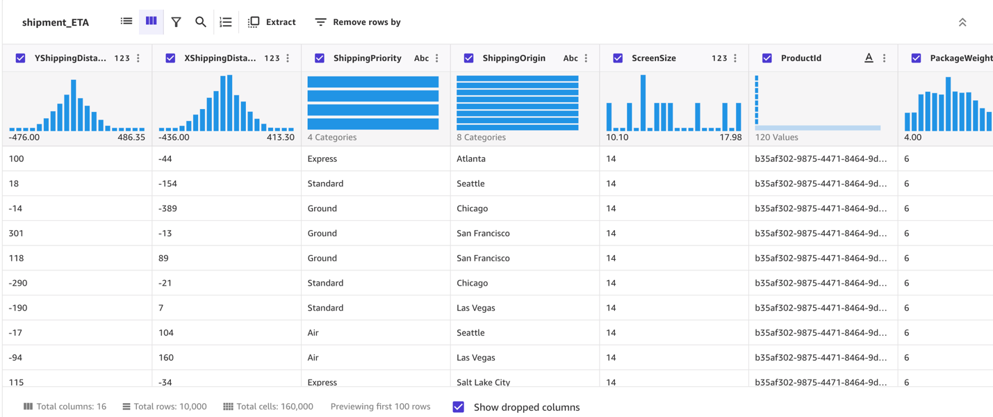
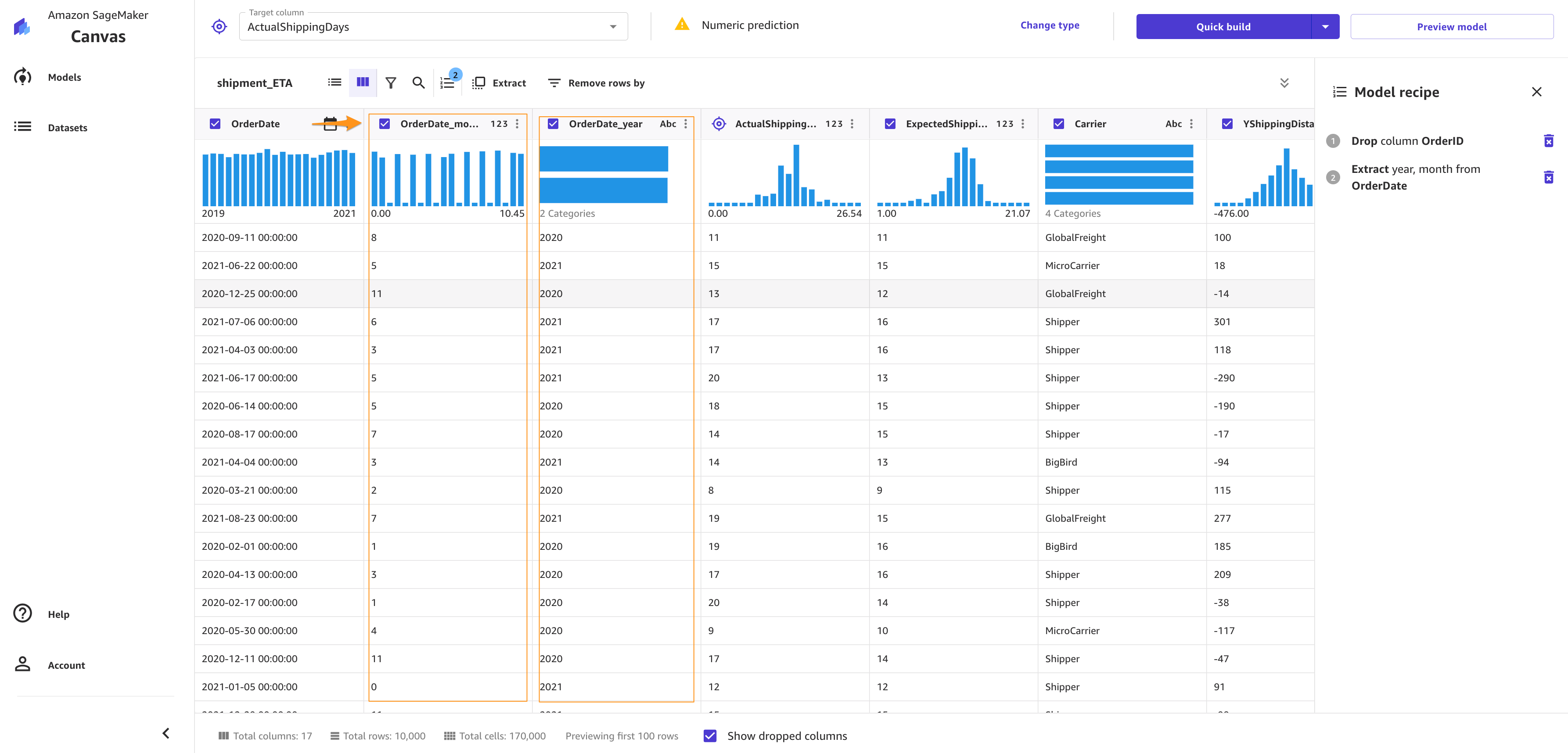
Grid view provides you with a graphical distribution of values for each column and the sample data. You can start inferring relevant columns for the training the model.

Let’s preview the model to see the estimated RMSE (root mean squared error) for this numeric prediction.

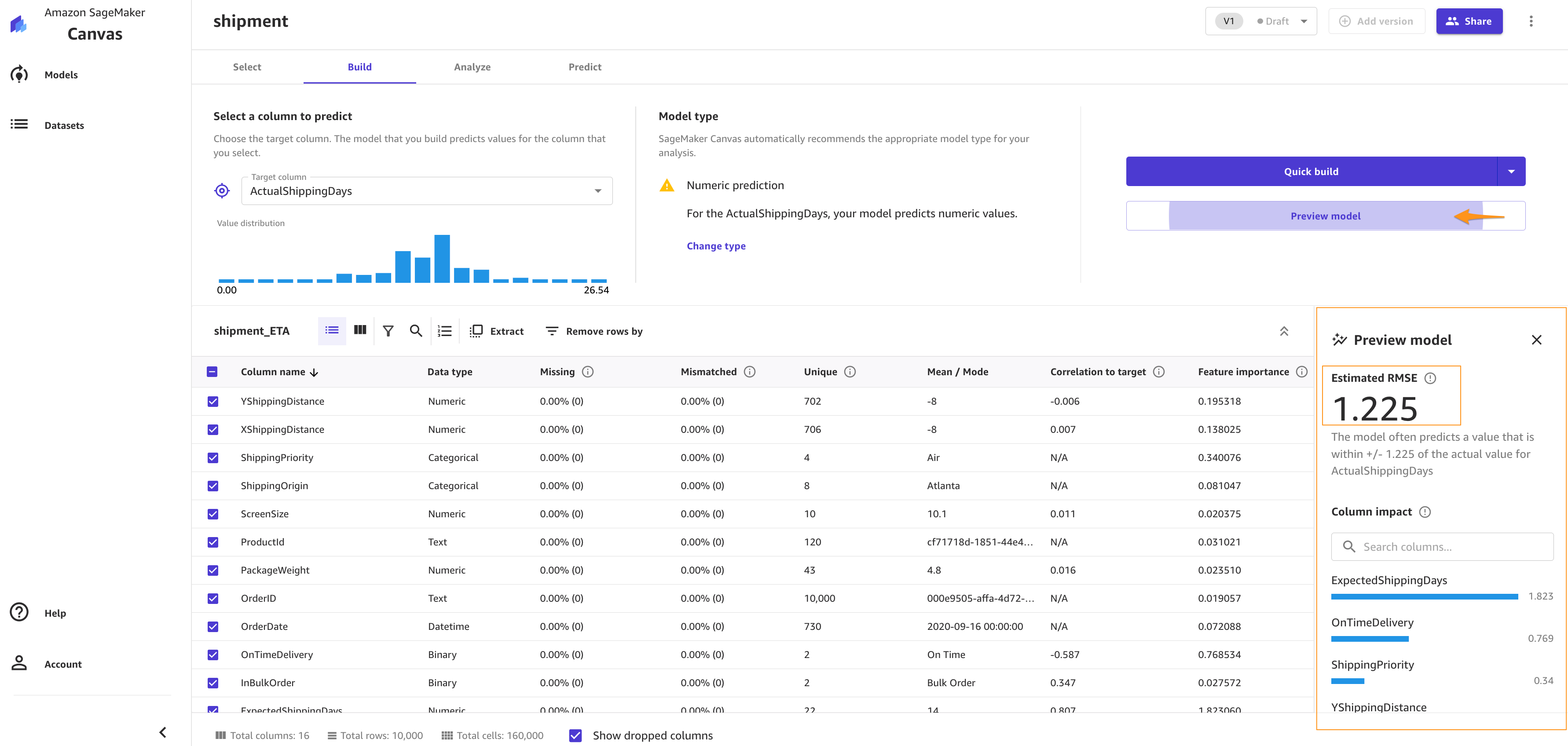
You can also drop some of the columns, if you don’t want to use them for the prediction, by simply deselecting them. For this post, we deselect the order*_**id* column. Because it’s a primary key, it doesn’t have valuable information, and so doesn’t add value to the model training process.

You can choose Preview model to get insights on feature importance and iterate the model quickly. We also see the RMSE is now 1.223, which is improved from 1.225. The lower the RMSE, the better a given model is able to fit a dataset.

From our exploratory data analysis, we can see that the dataset doesn’t have a lot of missing values. Therefore, we don’t have to handle missing values. If you see a lot of missing values for your features, you can filter the missing values.

To extract more insights, you can proceed with a datetime extraction. With the datetime extraction transform, you can extract values from a datetime column to a separate column.

To perform a datetime extraction, complete the following steps:

1. On the Build tab of the SageMaker Canvas application, choose Extract.
2. Choose the column from which you want to extract values (for this post, OrderDate).
3. For Value, choose one or more values to extract from the column. For this post, we choose Year and Month.The values you can extract from a timestamp column are Year, Month, Day, Hour, Week of year, Day of year, and Quarter.
4. Choose Add to add the transform to the model recipe.
   

SageMaker Canvas creates a new column in the dataset for each of the values you extract.

Model training

It’s time to finally train the model! Before building a complete model, it’s a good practice to have a general idea about the performances that our model will have by training a quick model. A quick model trains fewer combinations of models and hyperparameters in order to prioritize speed over accuracy. This is helpful in cases like ours where we want to prove the value of training an ML model for our use case. Note that the quick build option isn’t available for models bigger than 50,000 rows.

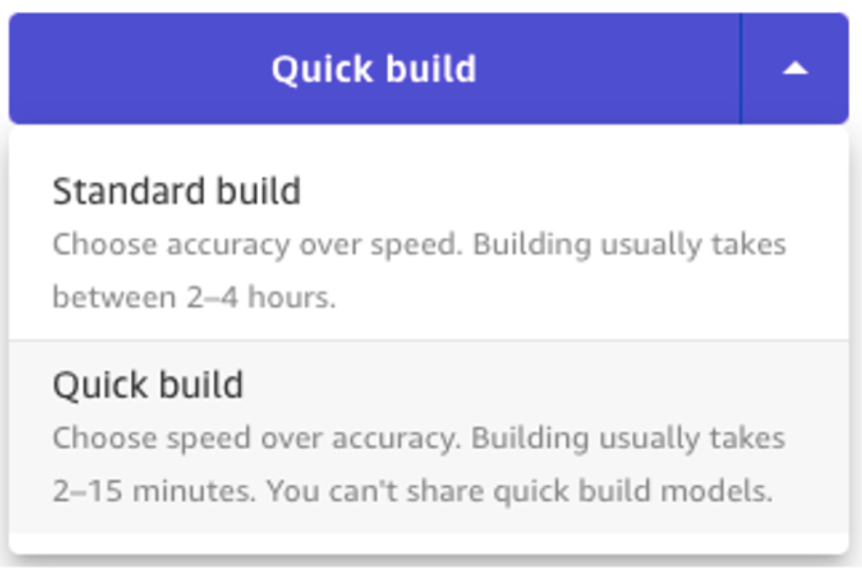
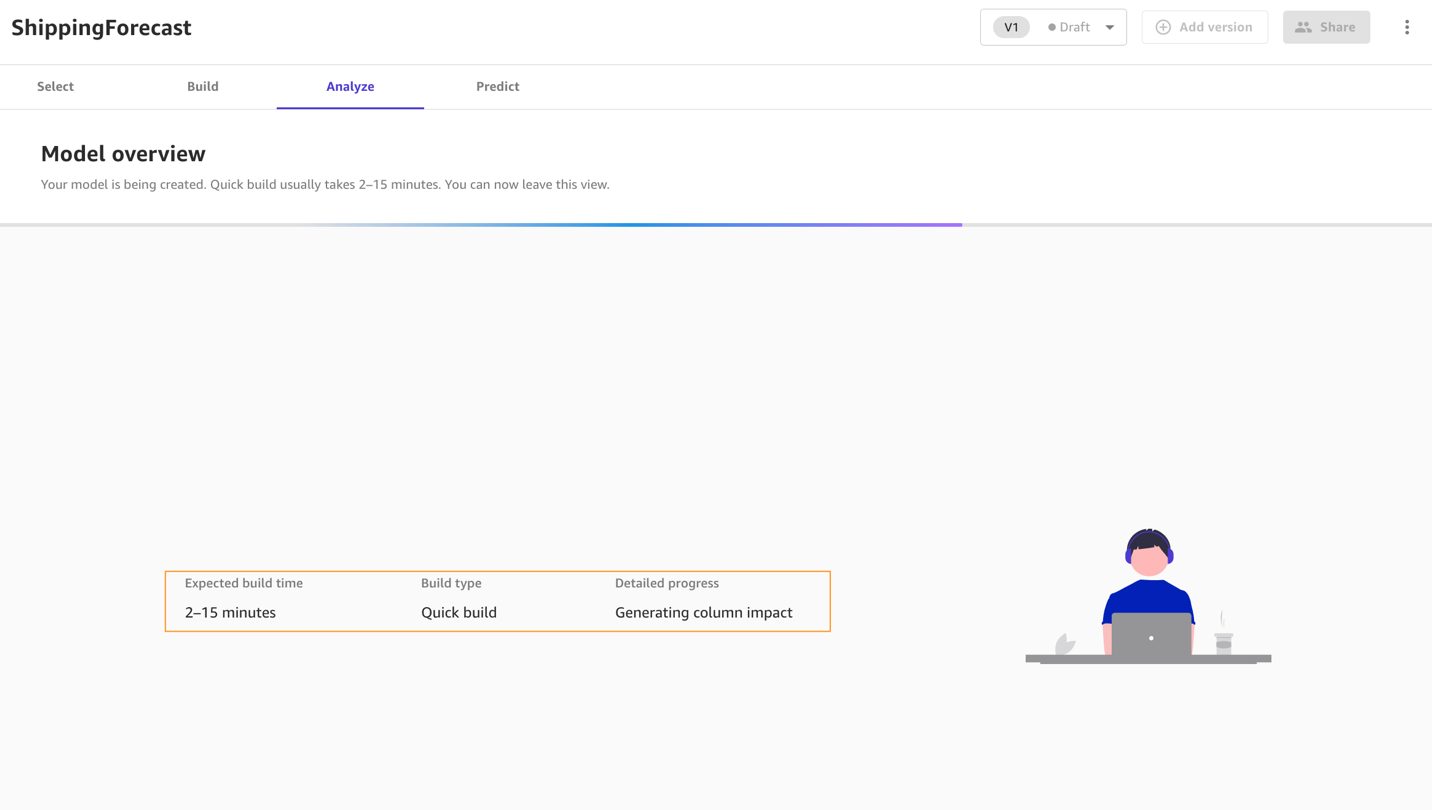
Now we wait anywhere from 2–15 minutes for the quick build to finish training our model.

Evaluate model performance

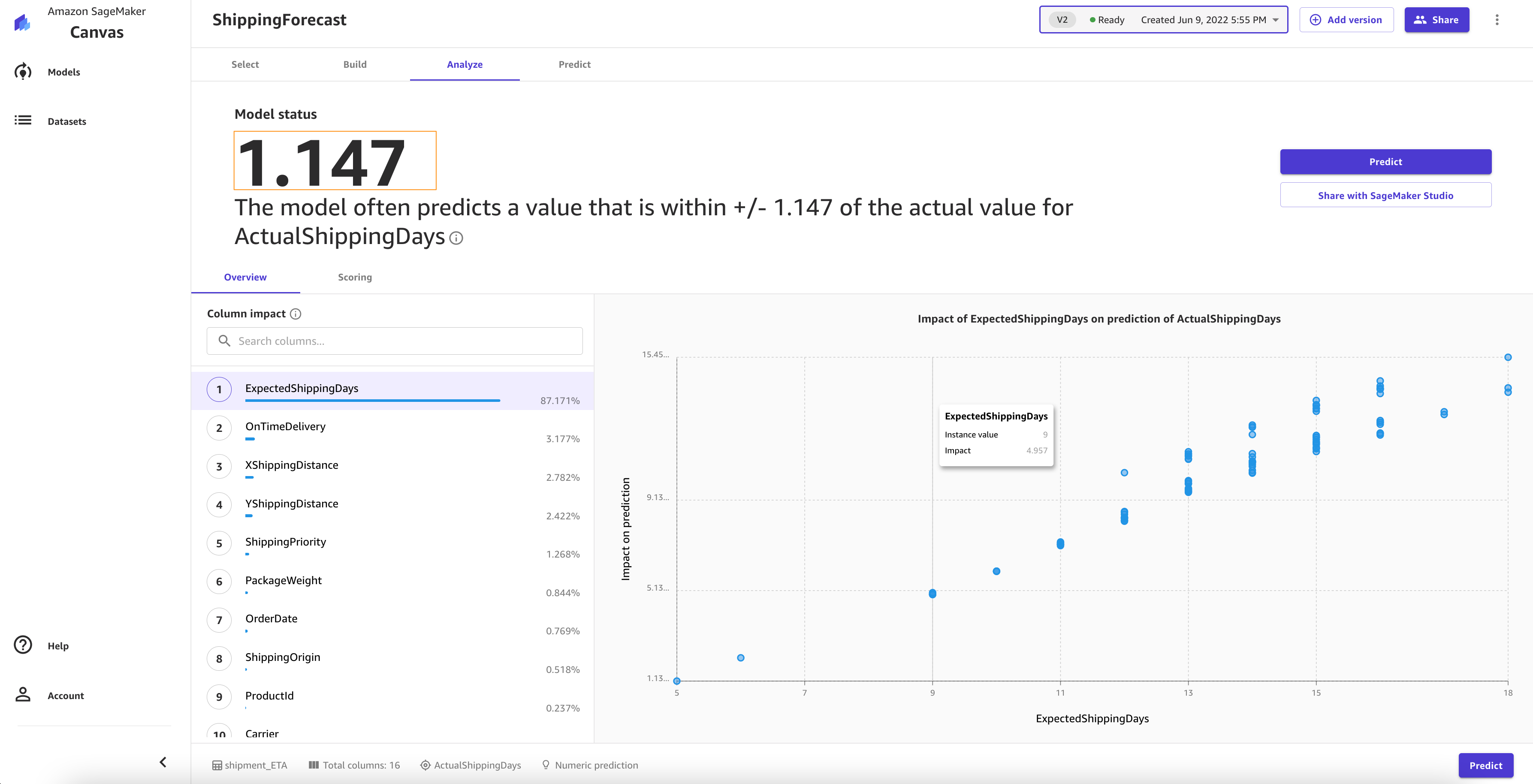
When training is complete, SageMaker Canvas automatically moves to the Analyze tab to show us the results of our quick training, as shown in the following screenshot.

You may experience slightly different values. This is expected. Machine learning introduces some variation in the process of training models, which can lead to different results for different builds.

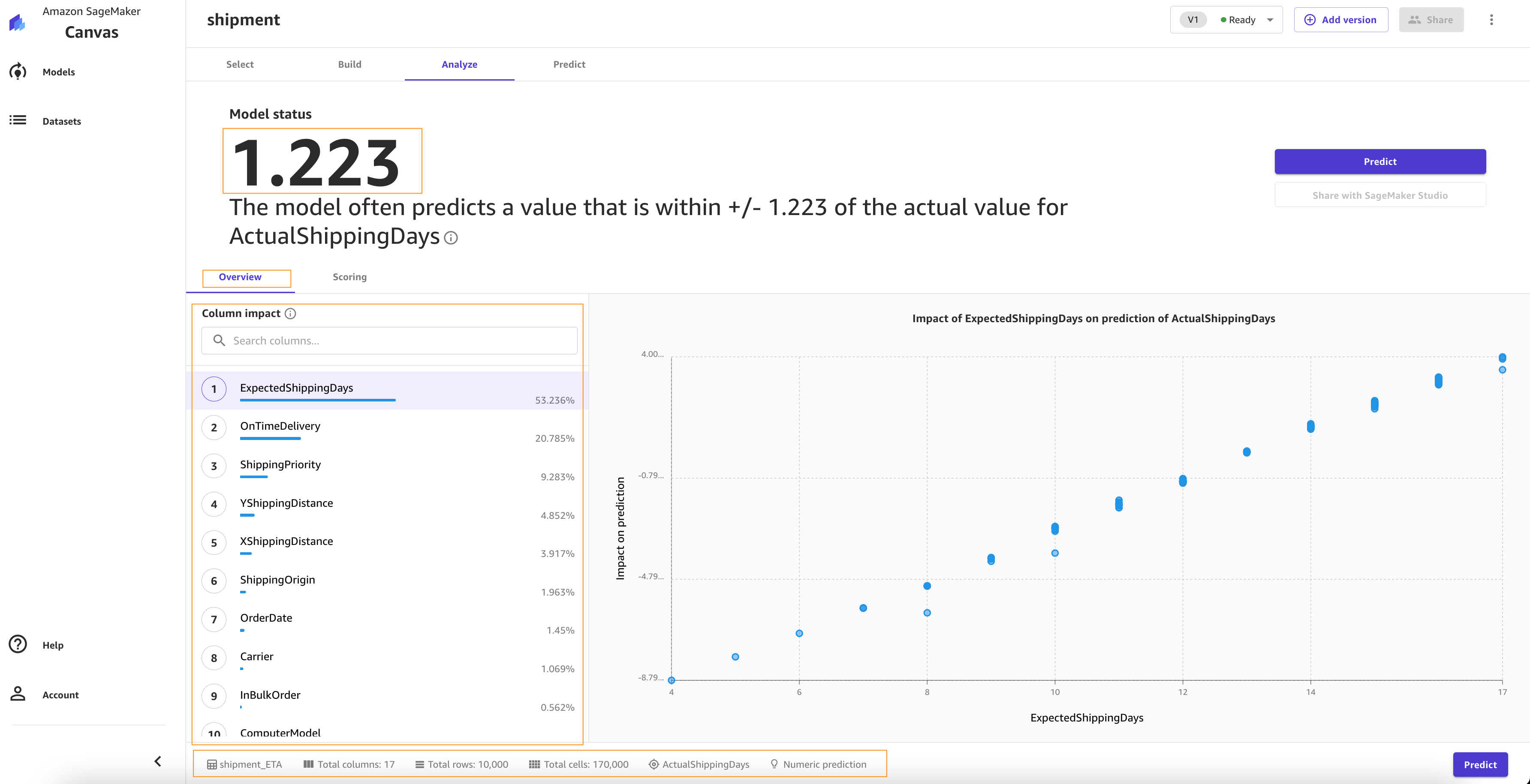
Let’s focus on the Overview tab. This tab shows you the column impact, or the estimated importance of each column in predicting the target column. In this example, the ExpectedShippingDays column has the most significant impact in our predictions.

On the Scoring tab, you can see a plot representing the best fit regression line for ActualshippingDays. On average, the model prediction has a difference of +/- 0.7 from the actual value of ActualShippingDays. The Scoring section for numeric prediction shows a line to indicate the model’s predicted value in relation to the data used to make predictions. The values of the numeric prediction are often +/- the RMSE value. The value that the model predicts is often within the range of the RMSE. The width of the purple band around the line indicates the RMSE range. The predicted values often fall within the range.

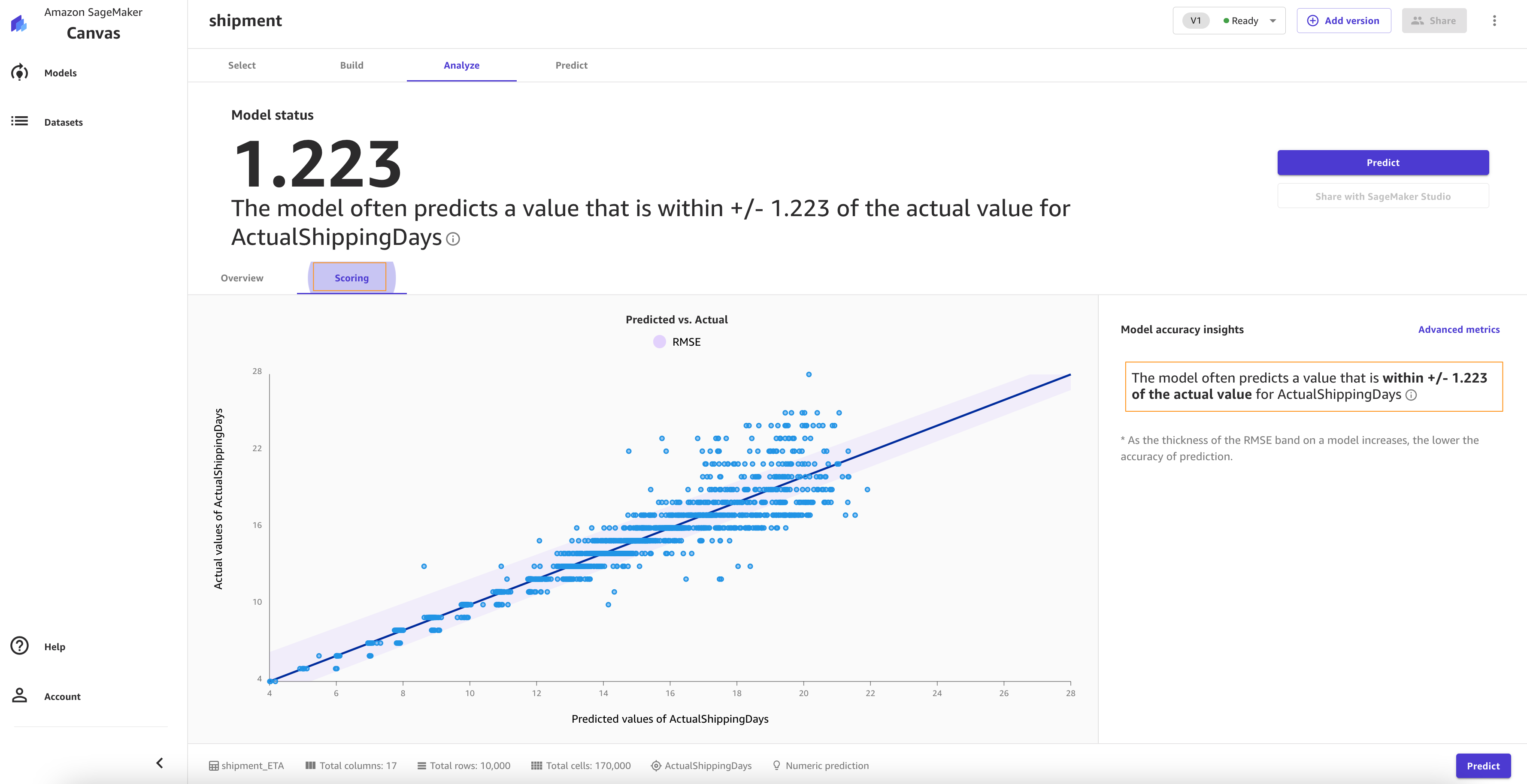
As the thickness of the RMSE band on a model increases, the accuracy of the prediction decreases. As you can see, the model predicts with high accuracy to begin with (lean band) and as the value of actualshippingdays increases (17–22), the band becomes thicker, indicating lower accuracy.

The Advanced metrics section contains information for users that want a deeper understanding of their model performance. The metrics for numeric prediction are as follows:

• R2 – The percentage of the difference in the target column that can be explained by the input column.
• MAE – Mean absolute error. On average, the prediction for the target column is +/- {MAE} from the actual value.
• MAPE – Mean absolute percent error. On average, the prediction for the target column is +/- {MAPE} % from the actual value.
• RMSE – Root mean square error. The standard deviation of the errors.

The following screenshot shows a graph of the residuals or errors. The horizontal line indicates an error of 0 or a perfect prediction. The blue dots are the errors. Their distance from the horizontal line indicates the magnitude of the errors.

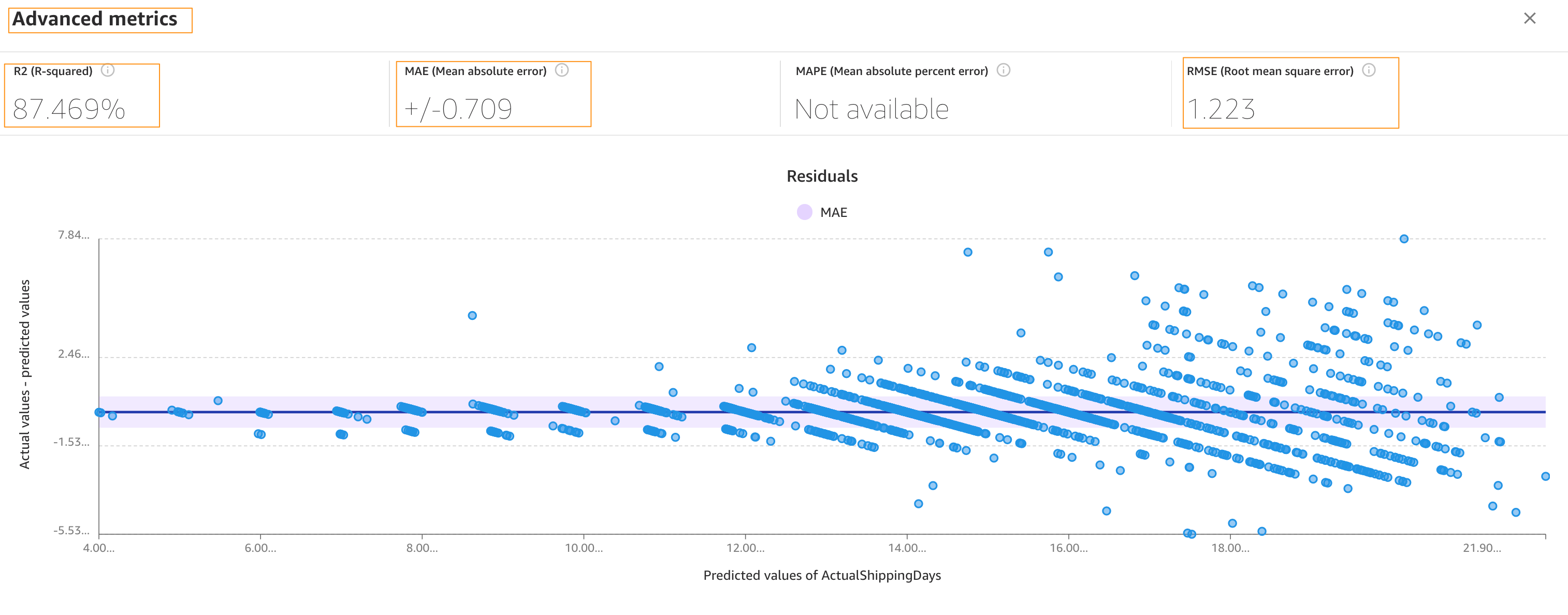
R-squared is a statistical measure of how close the data is to the fitted regression line. The higher percentage indicates that the model explains all the variability of the response data around its mean 87% of the time.

On average, the prediction for the target column is +/- 0.709 {MAE} from the actual value. This indicates that on average the model will predict the target within half a day. This is useful for planning purposes.

The model has a standard deviation (RMSE) of 1.223. As you can see, the model predicts with high accuracy to begin with (lean band) and as the value of actualshippingdays increases (17–22), the band becomes thicker, indicating lower accuracy.

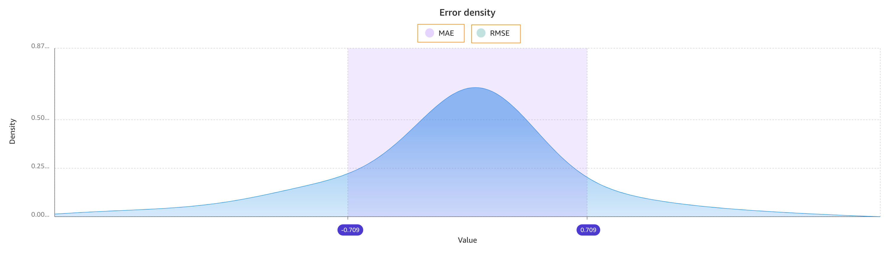
The following image shows an error density plot.

You now have two options as next steps:

• You can use this model to run some predictions by choosing Predict.
• You can create a new version of this model to train with the Standard build option. This will take much longer—about 4–6 hours—but will produce more accurate results.

Because we feel confident about using this model given the performances we’ve seen, we opt to go ahead and use the model for predictions. If you weren’t confident, you could have a data scientist review the modeling SageMaker Canvas did and offer potential improvements.

Note that training a model with the Standard build option is necessary to share the model with a data scientist with the Amazon SageMaker Studio integration.

Generate predictions

Now that the model is trained, let’s generate some predictions.

1. Choose Predict on the Analyze tab, or choose the Predict tab.
2. Choose Batch prediction.
3. Choose Select dataset, and choose the dataset ConsolidatedShipping.csv.

SageMaker Canvas uses this dataset to generate our predictions. Although it’s generally not a good idea not to use the same dataset for both training and testing, we’re using the same dataset for the sake of simplicity. You can also import another dataset if you desire.

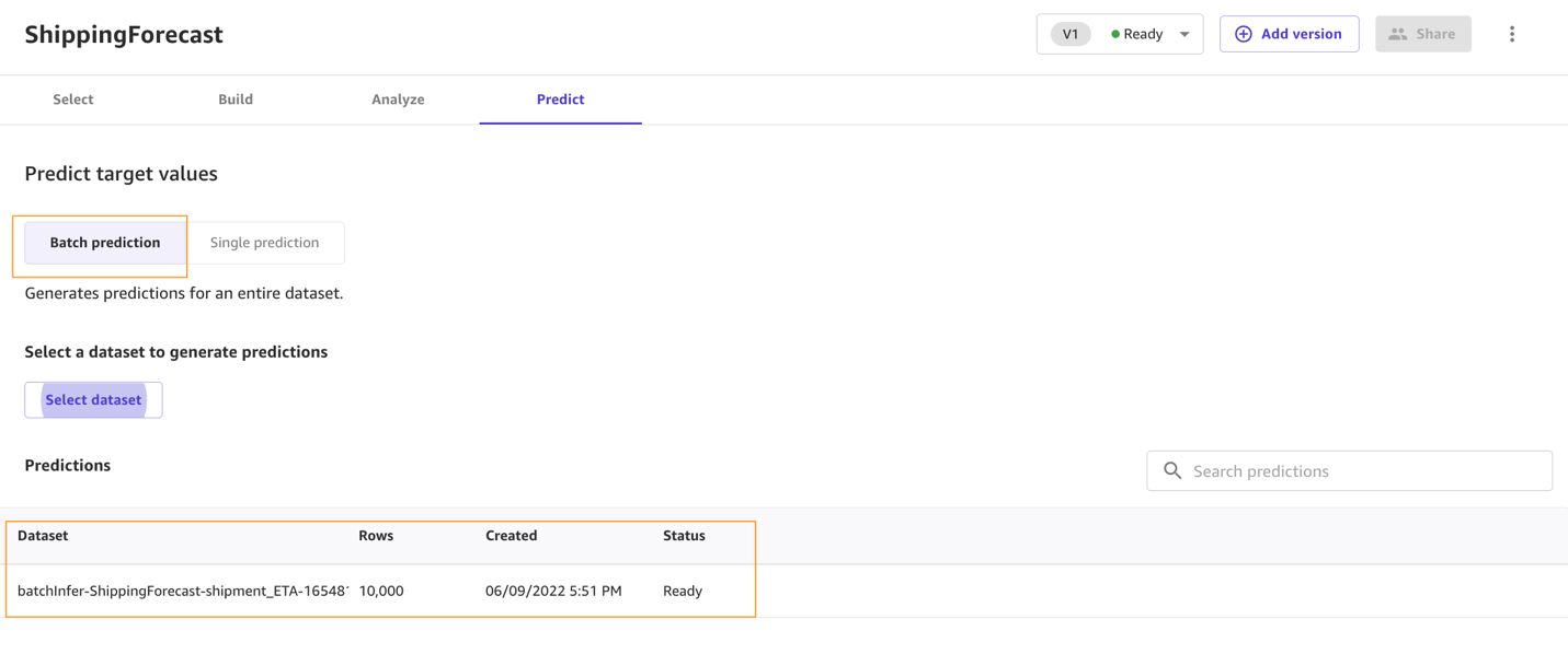
After a few seconds, the prediction is done and you can choose the eye icon to see a preview of the predictions, or choose Download to download a CSV file containing the full output.

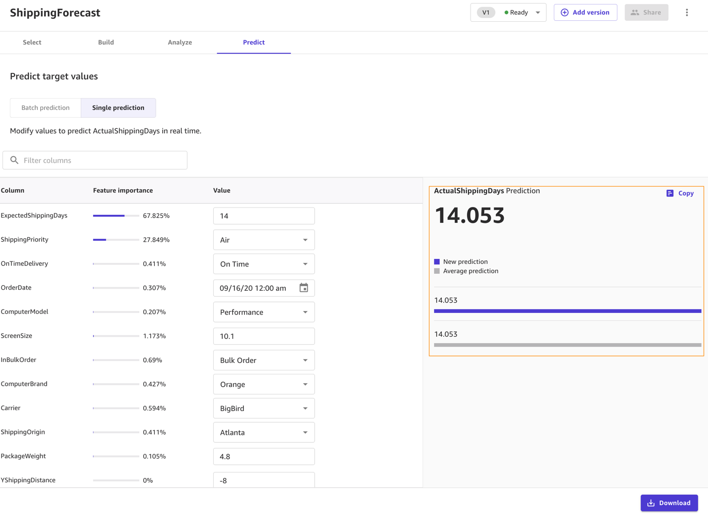
You can also choose to predict values one by one by selecting Single prediction instead of Batch prediction. SageMaker Canvas then shows you a view where you can provide the values for each feature manually and generate a prediction. This is ideal for situations like what-if scenarios—for example, how does ActualShippingDays change if the ShippingOrigin is Houston? What if we used a different carrier? What if the PackageWeight is different?

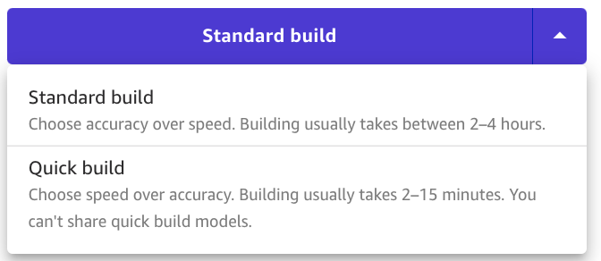
Standard build

Standard build chooses accuracy over speed. If you want to share the artifacts of the model with your data scientist and ML engineers, you may choose to create a standard build next.

First add a new version.

Then choose Standard build.

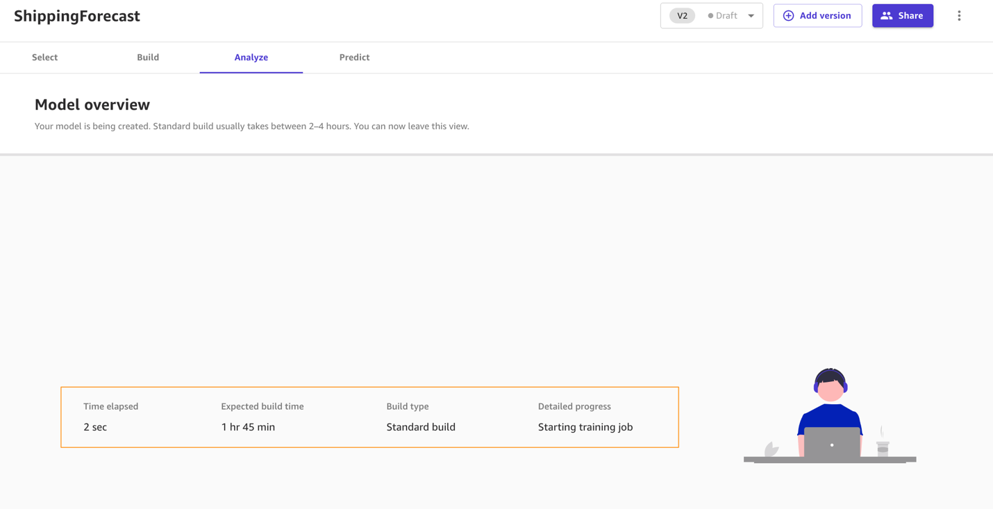
The Analyze tab shows your build progress.

When the model is complete, you can observe that the RMSE value of the standard build is 1.147, compared to 1.223 with the quick build.

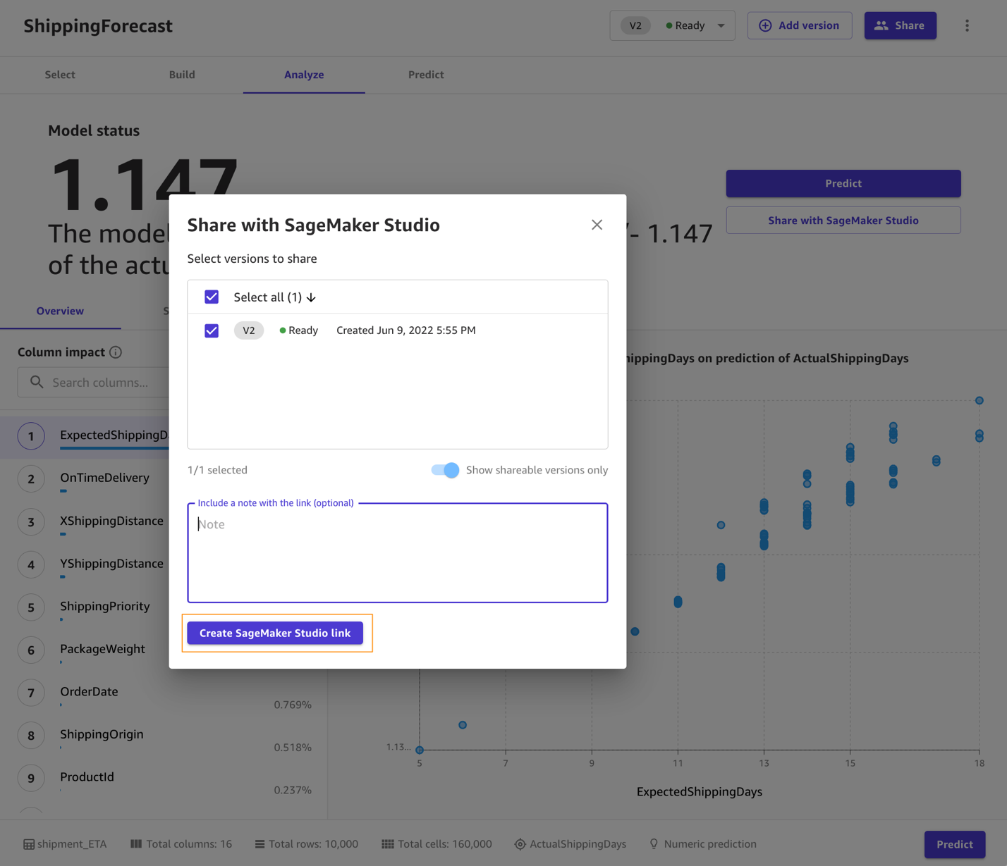
After you create a standard build, you can share the model with data scientists and ML engineers for further evaluation and iteration.

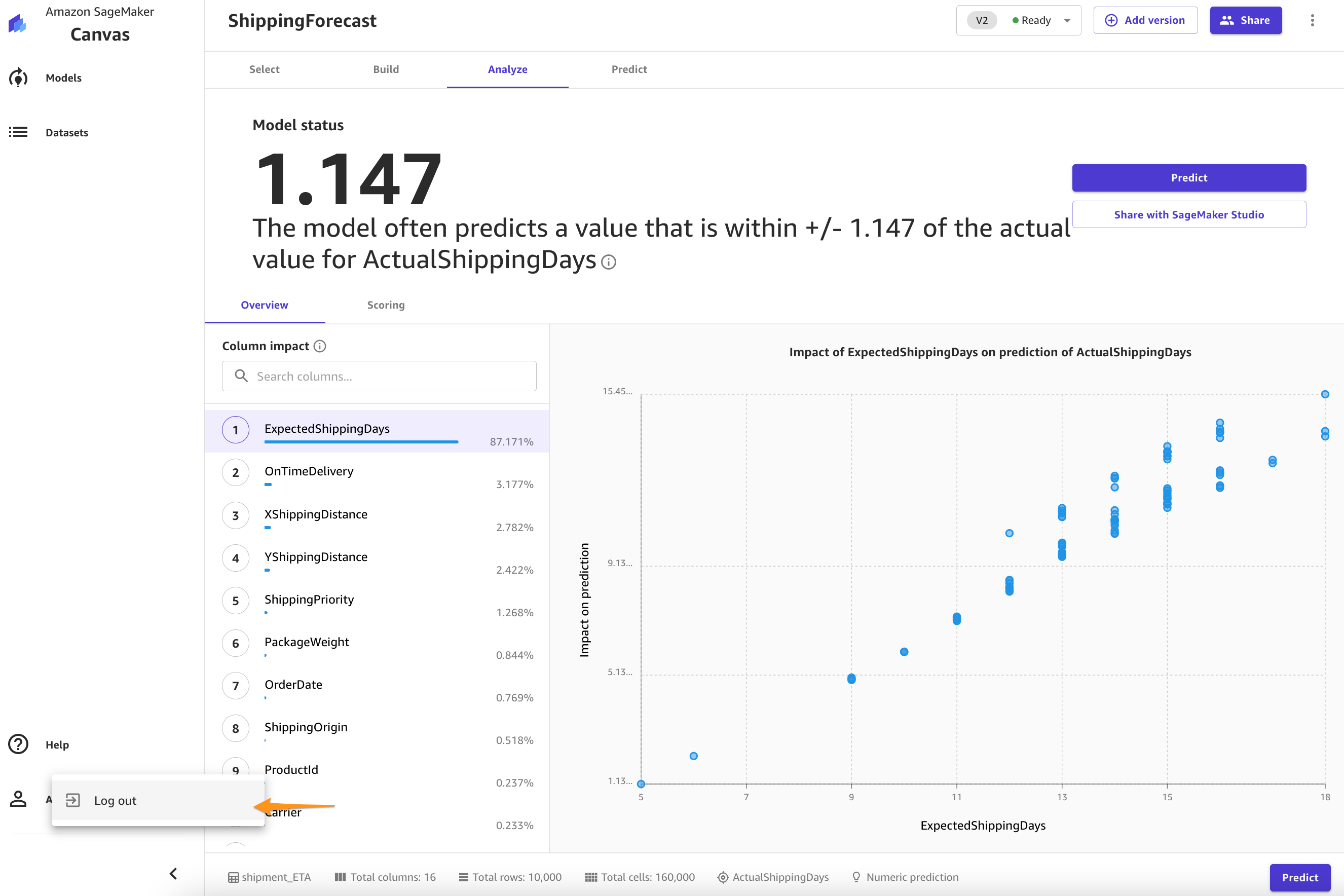
Clean up

To avoid incurring future session charges, log out of SageMaker Canvas.

Conclusion

In this post, we showed how a business analyst can create a shipment ETA prediction model with SageMaker Canvas using sample data. SageMaker Canvas allows you to create accurate ML models and generate predictions using a no-code, visual, point-and-click interface. Analysts can take this to the next level by sharing their models with data scientist colleagues. The data scientists can view the SageMaker Canvas model in Studio, where they can explore the choices SageMaker Canvas made to generate ML models, validate model results, and even take the model to production with a few clicks. This can accelerate ML-based value creation and help scale improved outcomes faster.

• To learn more about using SageMaker Canvas, see Build, Share, Deploy: how business analysts and data scientists achieve faster time-to-market using no-code ML and Amazon SageMaker Canvas.
• For more information about creating ML models with a no-code solution, see Announcing Amazon SageMaker Canvas – a Visual, No Code Machine Learning Capability for Business Analysts.

About the authors

Rajakumar Sampathkumar is a Principal Technical Account Manager at AWS, providing customers guidance on business-technology alignment and supporting the reinvention of their cloud operation models and processes. He is passionate about the cloud and machine learning. Raj is also a machine learning specialist and works with AWS customers to design, deploy, and manage their AWS workloads and architectures.

Meenakshisundaram Thandavarayan is a Senior AI/ML specialist with a passion to design, create and promote human-centered Data and Analytics experiences. He supports AWS Strategic customers on their transformation towards data driven organization.

Read More

This is a guest post co-written with Mutisya Ndunda from Trumid.

Like many industries, the corporate bond market doesn’t lend itself to a one-size-fits-all approach. It’s vast, liquidity is fragmented, and institutional clients demand solutions tailored to their specific needs. Advances in AI and machine learning (ML) can be employed to improve the customer experience, increase the efficiency and accuracy of operational workflows, and enhance performance by supporting multiple aspects of the trading process.

Trumid is a financial technology company building tomorrow’s credit trading network—a marketplace for efficient trading, information dissemination, and execution between corporate bond market participants. Trumid is optimizing the credit trading experience by combining leading-edge product design and technology principles with deep market expertise. The result is an integrated trading solution delivering a full ecosystem of protocols and execution tools within one intuitive platform.

The bond trading market has traditionally involved offline buyer/seller matching processes aided by rules-based technology. Trumid has embarked on an initiative to transform this experience. Through its electronic trading platform, traders can access thousands of bonds to buy or sell, a community of engaged users to interact with, and a variety of trading protocols and execution solutions. With an expanding network of users, Trumid’s AI and Data Strategy team partnered with the AWS Machine Learning Solutions Lab. The objective was to develop ML systems that could deliver a more personalized trading experience by modeling the interest and preferences of users for bonds available on Trumid.

These ML models can be used to speed up time to insight and action by personalizing how information is displayed to each user to ensure that the most relevant and actionable information a trader may care about is prioritized and accessible.

To solve this challenge, Trumid and the ML Solutions Lab developed an end-to-end data preparation, model training, and inference process based on a deep neural network model built using the Deep Graph Library for Knowledge Embedding (DGL-KE). An end-to-end solution with Amazon SageMaker was also deployed.

Benefits of graph machine learning

Real-world data is complex and interconnected, and often contains network structures. Examples include molecules in nature, social networks, the internet, roadways, and financial trading platforms.

Graphs provide a natural way to model this complexity by extracting important and rich information that is embedded in the relations between entities.

Traditional ML algorithms require data to be organized as tables or sequences. This generally works well, but some domains are more naturally and effectively represented by graphs (such as a network of objects related to each other, as illustrated later in this post). Instead of coercing these graph datasets into tables or sequences, you can use graph ML algorithms to both represent and learn from the data as presented in its graph form, including information about constituent nodes, edges, and other features.

Considering that bond trading is inherently represented as a network of interactions between buyers and sellers involving various types of bond instruments, an effective solution needs to harness the network effects of the communities of traders that participate in the market. Let’s look at how we leveraged the trading network effects and implemented this vision here.

Solution

Bond trading is characterized by several factors, including trade size, term, issuer, rate, coupon values, bid/ask offer, and type of trading protocol involved. In addition to orders and trades, Trumid also captures “indications of interest” (IOIs). The historical interaction data embodies the trading behavior and the market conditions evolving over time. We used this data to build a graph of timestamped interactions between traders, bonds, and issuers, and used graph ML to predict future interactions.

The recommendation solution comprised four main steps:

• Preparing the trading data as a graph dataset
• Training a knowledge graph embedding model
• Predicting new trades
• Packaging the solution as a scalable workflow

In the following sections, we discuss each step in more detail.

Preparing the trading data as a graph dataset

There are many ways to represent trading data as a graph. One option is to represent the data exhaustively with nodes, edges, and properties: traders as nodes with properties (such as employer or tenure), bonds as nodes with properties (issuer, amount outstanding, maturity, rate, coupon value), and trades as edges with properties (date, type, size). Another option is to simplify the data and use only nodes and relations (relations are typed edges like traded or issued-by). This latter approach worked better in our case, and we used the graph represented in the following figure.

Graph of relations between traders, bonds and bond issuers

Additionally, we removed some of the edges considered obsolete: if a trader interacted with more than 100 different bonds, we kept only the last 100 bonds.

Finally, we saved the graph dataset as a list of edges in TSV format:

t987	trade-old		i55198
t995	trade-old		i55306
t987	trade-recent	i24528
t995	trade-recent	i49181
t987	ioi-recent		i24523
t995	ioi-old 		i49178
…
i49611	issued-by		XXX
i46569	issued-by		YYY
i46507	issued-by		ZZZ

Training a knowledge graph embedding model

For graphs composed only of nodes and relations (often called knowledge graphs), the DGL team developed the knowledge graph embedding framework DGL-KE. KE stands for knowledge embedding, the idea being to represent nodes and relations (knowledge) by coordinates (embeddings) and optimize (train) the coordinates so that the original graph structure can be recovered from the coordinates. In the list of available embedding models, we selected TransE (translational embeddings). TransE trains embeddings with the objective of approximating the following equality:

Source node embedding + relation embedding = target node embedding (1)

We trained the model by invoking the dglke_train command. The output of the training is a model folder containing the trained embeddings.

For more details about TransE, refer to Translating Embeddings for Modeling Multi-relational Data.

Predicting new trades

To predict new trades from a trader with our model, we used the equality (1): add the trader embedding to the trade-recent embedding and looked for bonds closest to the resulting embedding.

We did this in two steps:

1. Compute scores for all possible trade-recent relations with dglke_predict.
2. Compute the top 100 highest scores for each trader.

For detailed instructions on how to use the DGL-KE, refer to Training knowledge graph embeddings at scale with the Deep Graph Library and DGL-KE Documentation.

Packaging the solution as a scalable workflow

We used SageMaker notebooks to develop and debug our code. For production, we wanted to invoke the model as a simple API call. We found that we didn’t need to separate data preparation, model training, and prediction, and it was convenient to package the whole pipeline as a single script and use SageMaker processing. SageMaker processing allows you to run a script remotely on a chosen instance type and Docker image without having to worry about resource allocation and data transfer. This was simple and cost-effective for us, because the GPU instance is only used and paid for during the 15 minutes needed for the script to run.

For detailed instructions on how to use SageMaker processing, see Amazon SageMaker Processing – Fully Managed Data Processing and Model Evaluation and Processing.

Results

Our custom graph model performed very well compared to other methods: performance improved by 80%, with more stable results across all trader types. We measured performance by mean recall (percentage of actual trades predicted by the recommender, averaged over all traders). With other standard metrics, the improvement ranged from 50–130%.

This performance enabled us to better match traders and bonds, indicating an enhanced trader experience within the model, with machine learning delivering a big step forward from hard-coded rules, which can be difficult to scale.

Conclusion

Trumid is focused on delivering innovative products and workflow efficiencies to their community of users. Building tomorrow’s credit trading network requires continuous collaboration with peers and industry experts like the AWS ML Solutions Lab, designed to help you innovate faster.

For more information, see the following resources:

• For a background on graph ML and use cases, refer to How AWS uses graph neural networks to meet customer needs.
• For more information about graph ML tools, explore DGL-KE, DGL, and Amazon Neptune.
• Deliver product recommendations with Amazon Personalize.
• Collaborate with the AWS Machine Learning Solutions Lab.

About the authors

Marc van Oudheusden is a Senior Data Scientist with the Amazon ML Solutions Lab team at Amazon Web Services. He works with AWS customers to solve business problems with artificial intelligence and machine learning. Outside of work you may find him at the beach, playing with his children, surfing or kitesurfing.

Mutisya Ndunda is the Head of Data Strategy and AI at Trumid. He is a seasoned financial professional with over 20 years of broad institutional experience in capital markets, trading, and financial technology.  Mutisya has a strong quantitative and analytical background with over a decade of experience in artificial intelligence, machine learning and big data analytics. Prior to Trumid, he was the CEO of Alpha Vertex, a financial technology company offering analytical solutions powered by proprietary AI algorithms to financial institutions. Mutisya holds a bachelor’s degree in Electrical Engineering from Cornell University and a master’s degree in Financial Engineering from Cornell University.

Isaac Privitera is a Senior Data Scientist at the Amazon Machine Learning Solutions Lab, where he develops bespoke machine learning and deep learning solutions to address customers’ business problems. He works primarily in the computer vision space, focusing on enabling AWS customers with distributed training and active learning.

Read More

The process of building a machine learning (ML) model is iterative until you find the candidate model that is performing well and is ready to be deployed. As data scientists iterate through that process, they need a reliable method to easily track experiments to understand how each model version was built and how it performed.

Amazon SageMaker allows teams to take advantage of a broad range of features to quickly prepare, build, train, deploy, and monitor ML models. Amazon SageMaker Pipelines provides a repeatable process for iterating through model build activities, and is integrated with Amazon SageMaker Experiments. By default, every SageMaker pipeline is associated with an experiment, and every run of that pipeline is tracked as a trial in that experiment. Then your iterations are automatically tracked without any additional steps.

In this post, we take a closer look at the motivation behind having an automated process to track experiments with Experiments and the native capabilities built into Pipelines.

Why is it important to keep your experiments organized?

Let’s take a step back for a moment and try to understand why it’s important to have experiments organized for machine learning. When data scientists approach a new ML problem, they have to answer many different questions, from data availability to how they will measure model performance.

At the start, the process is full of uncertainty and is highly iterative. As a result, this experimentation phase can produce multiple models, each created from their own inputs (datasets, training scripts, and hyperparameters) and producing their own outputs (model artifacts and evaluation metrics). The challenge then is to keep track of all these inputs and outputs of each iteration.

Data scientists typically train many different model versions until they find the combination of data transformation, algorithm, and hyperparameters that results in the best performing version of a model. Each of these unique combinations is a single experiment. With a traceable record of the inputs, algorithms, and hyperparameters that were used by that trial, the data science team can find it easy to reproduce their steps.

Having an automated process in place to track experiments improves the ability to reproduce as well as deploy specific model versions that are performing well. The Pipelines native integration with Experiments makes it easy to automatically track and manage experiments across pipeline runs.

Benefits of SageMaker Experiments

SageMaker Experiments allows data scientists organize, track, compare, and evaluate their training iterations.

Let’s start first with an overview of what you can do with Experiments:

• Organize experiments – Experiments structures experimentation with a top-level entity called an experiment that contains a set of trials. Each trial contains a set of steps called trial components. Each trial component is a combination of datasets, algorithms, and parameters. You can picture experiments as the top-level folder for organizing your hypotheses, your trials as the subfolders for each group test run, and your trial components as your files for each instance of a test run.
• Track experiments – Experiments allows data scientists to track experiments. It offers the possibility to automatically assign SageMaker jobs to a trial via simple configurations and via the tracking SDKs.
• Compare and evaluate experiments – The integration of Experiments with Amazon SageMaker Studio makes it easy to produce data visualizations and compare different trials. You can also access the trial data via the Python SDK to generate your own visualization using your preferred plotting libraries.

To learn more about Experiments APIs and SDKs, we recommend the following documentation: CreateExperiment and Amazon SageMaker Experiments Python SDK.

If you want to dive deeper, we recommend looking into the amazon-sagemaker-examples/sagemaker-experiments GitHub repository for further examples.

Integration between Pipelines and Experiments

The model building pipelines that are part of Pipelines are purpose-built for ML and allow you to orchestrate your model build tasks using a pipeline tool that includes native integrations with other SageMaker features as well as the flexibility to extend your pipeline with steps run outside SageMaker. Each step defines an action that the pipeline takes. The dependencies between steps are defined by a direct acyclic graph (DAG) built using the Pipelines Python SDK. You can build a SageMaker pipeline programmatically via the same SDK. After a pipeline is deployed, you can optionally visualize its workflow within Studio.

Pipelines automatically integrate with Experiments by automatically creating an experiment and trial for every run. Pipelines automatically create an experiment and a trial for every run of the pipeline before running the steps unless one or both of these inputs are specified. While running the pipeline’s SageMaker job, the pipeline associates the trial with the experiment, and associates to the trial every trial component that is created by the job. Specifying your own experiment or trial programmatically allows you to fine-tune how to organize your experiments.

The workflow we present in this example consists of a series of steps: a preprocessing step to split our input dataset into train, test, and validation datasets; a tuning step to tune our hyperparameters and kick off training jobs to train a model using the XGBoost built-in algorithm; and finally a model step to create a SageMaker model from the best trained model artifact. Pipelines also offers several natively supported step types outside of what is discussed in this post. We also illustrate how you can track your pipeline workflow and generate metrics and comparison charts. Furthermore, we show how to associate the new trial generated to an existing experiment that might have been created before the pipeline was defined.

SageMaker Pipelines code

You can review and download the notebook from the GitHub repository associated with this post. We look at the Pipelines-specific code to understand it better.

Pipelines enables you to pass parameters at run time. Here we define the processing and training instance types and counts at run time with preset defaults:

base_job_prefix = "pipeline-experiment-sample"
model_package_group_name = "pipeline-experiment-model-package"

processing_instance_count = ParameterInteger(
  name="ProcessingInstanceCount", default_value=1
)

training_instance_count = ParameterInteger(
  name="TrainingInstanceCount", default_value=1
)

processing_instance_type = ParameterString(
  name="ProcessingInstanceType", default_value="ml.m5.xlarge"
)
training_instance_type = ParameterString(
  name="TrainingInstanceType", default_value="ml.m5.xlarge"
)

Next, we set up a processing script that downloads and splits the input dataset into train, test, and validation parts. We use SKLearnProcessor for running this preprocessing step. To do so, we define a processor object with the instance type and count needed to run the processing job.

Pipelines allows us to achieve data versioning in a programmatic way by using execution-specific variables like ExecutionVariables.PIPELINE_EXECUTION_ID, which is the unique ID of a pipeline run. We can, for example, create a unique key for storing the output datasets in Amazon Simple Storage Service (Amazon S3) that ties them to a specific pipeline run. For the full list of variables, refer to Execution Variables.

framework_version = "0.23-1"

sklearn_processor = SKLearnProcessor(
    framework_version=framework_version,
    instance_type=processing_instance_type,
    instance_count=processing_instance_count,
    base_job_name="sklearn-ca-housing",
    role=role,
)

process_step = ProcessingStep(
    name="ca-housing-preprocessing",
    processor=sklearn_processor,
    outputs=[
        ProcessingOutput(
            output_name="train",
            source="/opt/ml/processing/train",
            destination=Join(
                on="/",
                values=[
                    "s3://{}".format(bucket),
                    prefix,
                    ExecutionVariables.PIPELINE_EXECUTION_ID,
                    "train",
                ],
            ),
        ),
        ProcessingOutput(
            output_name="validation",
            source="/opt/ml/processing/validation",
            destination=Join(
                on="/",
                values=[
                    "s3://{}".format(bucket),
                    prefix,
                    ExecutionVariables.PIPELINE_EXECUTION_ID,
                    "validation",
                ],
            )
        ),
        ProcessingOutput(
            output_name="test",
            source="/opt/ml/processing/test",
            destination=Join(
                on="/",
                values=[
                    "s3://{}".format(bucket),
                    prefix,
                    ExecutionVariables.PIPELINE_EXECUTION_ID,
                    "test",
                ],
            )
        ),
    ],
    code="california-housing-preprocessing.py",
)

Then we move on to create an estimator object to train an XGBoost model. We set some static hyperparameters that are commonly used with XGBoost:

model_path = f"s3://{default_bucket}/{base_job_prefix}/ca-housing-experiment-pipeline"

image_uri = sagemaker.image_uris.retrieve(
    framework="xgboost",
    region=region,
    version="1.2-2",
    py_version="py3",
    instance_type=training_instance_type,
)

xgb_train = Estimator(
    image_uri=image_uri,
    instance_type=training_instance_type,
    instance_count=training_instance_count,
    output_path=model_path,
    base_job_name=f"{base_job_prefix}/ca-housing-train",
    sagemaker_session=sagemaker_session,
    role=role,
)

xgb_train.set_hyperparameters(
    eval_metric="rmse",
    objective="reg:squarederror",  # Define the object metric for the training job
    num_round=50,
    max_depth=5,
    eta=0.2,
    gamma=4,
    min_child_weight=6,
    subsample=0.7
)

We do hyperparameter tuning of the models we create by using a ContinuousParameter range for lambda. Choosing one metric to be the objective metric tells the tuner (the instance that runs the hyperparameters tuning jobs) that you will evaluate the training job based on this specific metric. The tuner returns the best combination based on the best value for this objective metric, meaning the best combination that minimizes the best root mean square error (RMSE).

objective_metric_name = "validation:rmse"

hyperparameter_ranges = {
    "lambda": ContinuousParameter(0.01, 10, scaling_type="Logarithmic")
}

tuner = HyperparameterTuner(estimator,
                            objective_metric_name,
                            hyperparameter_ranges,
                            objective_type=objective_type,
                            strategy="Bayesian",
                            max_jobs=10,
                            max_parallel_jobs=3)

tune_step = TuningStep(
    name="HPTuning",
    tuner=tuner_log,
    inputs={
        "train": TrainingInput(
            s3_data=process_step.properties.ProcessingOutputConfig.Outputs[
                "train"
            ].S3Output.S3Uri,
            content_type="text/csv",
        ),
        "validation": TrainingInput(
            s3_data=process_step.properties.ProcessingOutputConfig.Outputs[
                "validation"
            ].S3Output.S3Uri,
            content_type="text/csv",
        ),
    } 
)

The tuning step runs multiple trials with the goal of determining the best model among the parameter ranges tested. With the method get_top_model_s3_uri, we rank the top 50 performing versions of the model artifact S3 URI and only extract the best performing version (we specify k=0 for the best) to create a SageMaker model.

model_bucket_key = f"{default_bucket}/{base_job_prefix}/ca-housing-experiment-pipeline"
model_candidate = Model(
    image_uri=image_uri,
    model_data=tune_step.get_top_model_s3_uri(top_k=0, s3_bucket=model_bucket_key),
    sagemaker_session=sagemaker_session,
    role=role,
    predictor_cls=XGBoostPredictor,
)

create_model_step = CreateModelStep(
    name="CreateTopModel",
    model=model_candidate,
    inputs=sagemaker.inputs.CreateModelInput(instance_type="ml.m4.large"),
)

When the pipeline runs, it creates trial components for each hyperparameter tuning job and each SageMaker job created by the pipeline steps.

You can further configure the integration of pipelines with Experiments by creating a PipelineExperimentConfig object and pass it to the pipeline object. The two parameters define the name of the experiment that will be created, and the trial that will refer to the whole run of the pipeline.

If you want to associate a pipeline run to an existing experiment, you can pass its name, and Pipelines will associate the new trial to it. You can prevent the creation of an experiment and trial for a pipeline run by setting pipeline_experiment_config to None.

#Pipeline experiment config
ca_housing_experiment_config = PipelineExperimentConfig(
    experiment_name,
    Join(
        on="-",
        values=[
            "pipeline-execution",
            ExecutionVariables.PIPELINE_EXECUTION_ID
        ],
    )
)

We pass on the instance types and counts as parameters, and chain the preceding steps in order as follows. The pipeline workflow is implicitly defined by the outputs of a step being the inputs of another step.

pipeline_name = f"CAHousingExperimentsPipeline"

pipeline = Pipeline(
    name=pipeline_name,
    pipeline_experiment_config=ca_housing_experiment_config,
    parameters=[
        processing_instance_count,
        processing_instance_type,
        training_instance_count,
        training_instance_type
    ],
    steps=[process_step,tune_step,create_model_step],
)

The full-fledged pipeline is now created and ready to go. We add an execution role to the pipeline and start it. From here, we can go to the SageMaker Studio Pipelines console and visually track every step. You can also access the linked logs from the console to debug a pipeline.

pipeline.upsert(role_arn=sagemaker.get_execution_role())
execution = pipeline.start()

The preceding screenshot shows in green a successfully run pipeline. We obtain the metrics of one trial from a run of the pipeline with the following code:

# SM Pipeline injects the Execution ID into trial component names
execution_id = execution.describe()['PipelineExecutionArn'].split('/')[-1]
source_arn_filter = Filter(
    name="TrialComponentName", operator=Operator.CONTAINS, value=execution_id
)

source_type_filter = Filter(
    name="Source.SourceType", operator=Operator.EQUALS, value="SageMakerTrainingJob"
)

search_expression = SearchExpression(
    filters=[source_arn_filter, source_type_filter]
)

trial_component_analytics = ExperimentAnalytics(
    sagemaker_session=sagemaker_session,
    experiment_name=experiment_name,
    search_expression=search_expression.to_boto()
)

analytic_table = trial_component_analytics.dataframe()
analytic_table.head()

Compare the metrics for each trial component

You can plot the results of hyperparameter tuning in Studio or via other Python plotting libraries. We show both ways of doing this.

Explore the training and evaluation metrics in Studio

Studio provides an interactive user interface where you can generate interactive plots. The steps are as follows:

1. Choose Experiments and Trials from the SageMaker resources icon on the left sidebar.
2. Choose your experiment to open it.
3. Choose (right-click) the trial of interest.
4. Choose Open in trial component list.
5. Press Shift to select the trial components representing the training jobs.
6. Choose Add chart.
7. Choose New chart and customize it to plot the collected metrics that you want to analyze. For our use case, choose the following:
   1. For Data type¸ select Summary Statistics.
   2. For Chart type¸ select Scatter Plot.
   3. For X-axis, choose lambda.
   4. For Y-axis, choose validation:rmse_last.

The new chart appears at the bottom of the window, labeled as ‘8’.

You can include more or fewer training jobs by pressing Shift and choosing the eye icon for a more interactive experience.

Analytics with SageMaker Experiments

When the pipeline run is complete, we can quickly visualize how different variations of the model compare in terms of the metrics collected during training. Earlier, we exported all trial metrics to a Pandas DataFrame using ExperimentAnalytics. We can reproduce the plot obtained in Studio by using the Matplotlib library.

analytic_table.plot.scatter("lambda", "validation:rmse - Last", grid=True)

Conclusion

The native integration between SageMaker Pipelines and SageMaker Experiments allows data scientists to automatically organize, track, and visualize experiments during model development activities. You can create experiments to organize all your model development work, such as the following:

• A business use case you’re addressing, such as creating an experiment to predict customer churn
• An experiment owned by the data science team regarding marketing analytics, for example
• A specific data science and ML project

In this post, we dove into Pipelines to show how you can use it in tandem with Experiments to organize a fully automated end-to-end workflow.

As a next step, you can use these three SageMaker features – Studio, Experiments and Pipelines – for your next ML project.

Suggested readings

• Amazon SageMaker now supports cross-account lineage tracking and multi-hop lineage querying
• Announcing Amazon SageMaker Inference Recommender
• Introducing the Well-Architected Framework for Machine Learning
• Machine Learning Lens: AWS Well-Architected Framework
• Roundup of re:Invent 2021 Amazon SageMaker announcements

About the authors

Paolo Di Francesco is a solutions architect at AWS. He has experience in the telecommunications and software engineering. He is passionate about machine learning and is currently focusing on using his experience to help customers reach their goals on AWS, in particular in discussions around MLOps. Outside of work, he enjoys playing football and reading.

Mario Bourgoin is a Senior Partner Solutions Architect for AWS, an AI/ML specialist, and the global tech lead for MLOps. He works with enterprise customers and partners deploying AI solutions in the cloud. He has more than 30 years of experience doing machine learning and AI at startups and in enterprises, starting with creating one of the first commercial machine learning systems for big data. Mario spends his free time playing with his three Belgian Tervurens, cooking dinner for his family, and learning about mathematics and cosmology.

Ganapathi Krishnamoorthi is a Senior ML Solutions Architect at AWS. Ganapathi provides prescriptive guidance to startup and enterprise customers helping them to design and deploy cloud applications at scale. He is specialized in machine learning and is focused on helping customers leverage AI/ML for their business outcomes. When not at work, he enjoys exploring outdoors and listening to music.

Valerie Sounthakith is a Solutions Architect for AWS, working in the Gaming Industry and with Partners deploying AI solutions. She is aiming to build her career around Computer Vision. During her free time, Valerie spends it to travel, discover new food spots and change her house interiors.

Read More