Research over the past few years has shown that machine learning (ML) models are vulnerable to adversarial inputs, where an adversary can craft inputs to strategically alter the model’s output (in image classification, speech recognition, or fraud detection). For example, imagine you have deployed a model that identifies your employees based on images of their faces. As demonstrated in the whitepaper Accessorize to a Crime: Real and Stealthy Attacks on State-of-the-Art Face Recognition, malicious employees may apply subtle but carefully designed modifications to their image and fool the model to authenticate them as other employees. Obviously, such adversarial inputs—especially if there are a significant amount of them—can have a devastating business impact.
Ideally, we want to detect each time an adversarial input is sent to the model to quantify how adversarial inputs are impacting your model and business. To this end, a wide class of methods analyze individual model inputs to check for adversarial behavior. However, active research in adversarial ML has led to increasingly sophisticated adversarial inputs, many of which are known to make detection ineffective. The reason for this shortcoming is that it’s difficult to draw conclusions from an individual input as to whether it’s adversarial or not. To this end, a recent class of methods focuses on distributional-level checks by analyzing multiple inputs at a time. The key idea behind these new methods is that considering multiple inputs at a time enables more powerful statistical analysis that isn’t possible with individual inputs. However, in the face of a determined adversary with deep knowledge of the model, even these advanced detection methods can fail.
However, we can defeat even these determined adversaries by providing the defense methods with additional information. Specifically, instead of just the analyzing model inputs, analyzing the latent representations collected from the intermediate layers in a deep neural network significantly strengthens the defense.
In this post, we walk you through how to detect adversarial inputs using Amazon SageMaker Model Monitor and Amazon SageMaker Debugger for an image classification model hosted on Amazon SageMaker.
To reproduce the different steps and results listed in this post, clone the repository detecting-adversarial-samples-using-sagemaker into your Amazon SageMaker notebook instance and run the notebook.
Detecting adversarial inputs
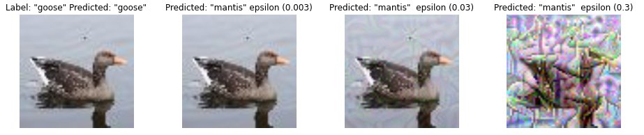
We show you how to detect adversarial inputs using the representations collected from a deep neural network. The following four images show the original training image on the left (taken from the Tiny ImageNet dataset) and three images produced by the Projected Gradient Descent (PGD) attack [1] with different perturbation parameters ϵ. The model used here was ResNet18. The ϵ parameter defines the amount of adversarial noise added to the images. The original image (left) is correctly predicted as class 67 (goose). The adversarially modified images 2, 3, and 4 are incorrectly predicted as class 51 (mantis) by the ResNet18 model. We can also see that images generated with small ϵ are perceptually indistinguishable from the original input image.
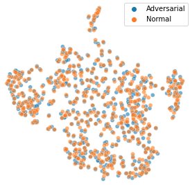
Next, we create a set of normal and adversarial images and use t-Distributed Stochastic Neighbor Embedding (t-SNE [2]) to visually compare their distributions. t-SNE is a dimensionality reduction method that maps high-dimensional data into a 2- or 3-dimensional space. Each data point in the following image presents an input image. Orange data points present the normal inputs taken from the test set, and blue data points indicate the corresponding adversarial images generated with an epsilon of 0.003. If normal and adversarial inputs are distinguishable, then we would expect separate clusters in the t-SNE visualization. Because both belong to the same cluster, this means that a detection technique that focuses solely on changes in the model input distribution can’t distinguish these inputs.
Let’s take a closer look at the layer representations produced by different layers in the ResNet18 model. ResNet18 consists of 18 layers; in the following image, we visualize the t-SNE embeddings for the representations for six of these layers.
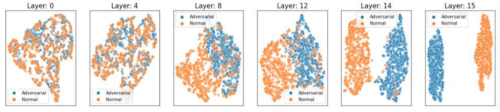
As the preceding figure shows, natural and adversarial inputs become more distinguishable for deeper layers of the ResNet18 model.
Based on these observations, we use a statistical method that measures distinguishability with hypothesis testing. The method consists of a two-sample test using maximum mean discrepancy (MMD). MMD is a kernel-based metric for measuring the similarity between two distributions generating the data. A two-sample test takes two sets that contain inputs drawn from two distributions, and determines whether these distributions are the same. We compare the distribution of inputs observed in the training data and compare it with the distribution of the inputs received during inference.
Our method uses these inputs to estimate the p-value using MMD. If the p-value is greater than a user-specific significance threshold (5% in our case), we conclude that both distributions are different. The threshold tunes the trade-off between false positives and false negatives. A higher threshold, such as 10%, decreases the false negative rate (there are fewer cases when both distributions were different but the test failed to indicate that). However, it also results in more false positives (the test indicates both distributions are different even when that isn’t the case). On the other hand, a lower threshold, such as 1%, results in fewer false positives but more false negatives.
Instead of applying this method solely on the raw model inputs (images), we use the latent representations produced by the intermediate layers of our model. To account for its probabilistic nature, we apply the hypothesis test 100 times on 100 randomly selected natural inputs and 100 randomly selected adversarial inputs. Then we report the detection rate as the percentage of tests that resulted in a detection event according to our 5% significance threshold. The higher detection rate is a stronger indication that the two distributions are different. This procedure gives us the following detection rates:
- Layer 1: 3%
- Layer 4: 7%
- Layer 8: 84%
- Layer 12: 95%
- Layer 14: 100%
- Layer 15: 100%
In the initial layers, the detection rate is rather low (less than 10%), but increases to 100% in the deeper layers. Using the statistical test, the method can confidently detect adversarial inputs in deeper layers. It is often sufficient to simply use the representations generated by the penultimate layer (the last layer before the classification layer in a model). For more sophisticated adversarial inputs, it’s useful to use representations from other layers and aggregate the detection rates.
Solution overview
In the previous section, we saw how to detect adversarial inputs using representations from the penultimate layer. Next, we show how to automate these tests on SageMaker by using Model Monitor and Debugger. For this example, we first train an image classification ResNet18 model on the tiny ImageNet dataset. Next, we deploy the model on SageMaker and create a custom Model Monitor schedule that runs the statistical test. Afterwards, we run inference with normal and adversarial inputs to see how effective the method is.
Capture tensors using Debugger
During model training, we use Debugger to capture representations generated by the penultimate layer, which are used later on to derive information about the distribution of normal inputs. Debugger is a feature of SageMaker that enables you to capture and analyze information such as model parameters, gradients, and activations during model training. These parameter, gradient, and activation tensors are uploaded to Amazon Simple Storage Service (Amazon S3) while the training is in progress. You can configure rules that analyze these for issues such as overfitting and vanishing gradients. For our use case, we only want to capture the penultimate layer of the model (.*avgpool_output) and the model outputs (predictions). We specify a Debugger hook configuration that defines a regular expression for the layer representations to be collected. We also specify a save_interval that instructs Debugger to collect this data during the validation phase every 100 forward passes. See the following code:
Run SageMaker training
We pass the Debugger configuration into the SageMaker estimator and start the training:
Deploy an image classification model
After the model training is complete, we deploy the model as an endpoint on SageMaker. We specify an inference script that defines the model_fn and transform_fn functions. These functions specify how the model is loaded and how incoming data needs to be preprocessed to perform the model inference. For our use case, we enable Debugger to capture relevant data during inference. In the model_fn function, we specify a Debugger hook and a save_config that specifies that for each inference request, the model inputs (images), the model outputs (predictions), and the penultimate layer are recorded (.*avgpool_output). We then register the hook on the model. See the following code:
Now we deploy the model, which we can do from the notebook in two ways. We can either call pytorch_estimator.deploy() or create a PyTorch model that points to the model artifact files in Amazon S3 that have been created by the SageMaker training job. In this post, we do the latter. This allows us to pass in environment variables into the Docker container, which is created and deployed by SageMaker. We need the environment variable tensors_output to tell the script where to upload the tensors that are collected by SageMaker Debugger during inference. See the following code:
Next, we deploy the predictor on an ml.m5.xlarge instance type:
Create a custom Model Monitor schedule
When the endpoint is up and running, we create a customized Model Monitor schedule. This is a SageMaker processing job that runs on a periodic interval (such as hourly or daily) and analyzes the inference data. Model Monitor provides a pre-configured container that analyzes and detects data drift. In our case, we want to customize it to fetch the Debugger data and run the MMD two-sample test on the retrieved layer representations.
To customize it, we first define the Model Monitor object, which specifies on which instance type these jobs are going to run and the location of our custom Model Monitor container:
We want to run this job on an hourly basis, so we specify CronExpressionGenerator.hourly() and the output locations where analysis results are uploaded to. For that we need to define ProcessingOutput for the SageMaker processing output:
Let’s look closer at what our custom Model Monitor container is running. We create an evaluation script, which loads the data captured by Debugger. We also create a trial object, which enables us to access, query, and filter the data that Debugger saved. With the trial object, we can iterate over the steps saved during the inference and training phases trial.steps(mode).
First, we fetch the model outputs (trial.tensor("ResNet_output_0")) as well as the penultimate layer (trial.tensor_names(regex=".*avgpool_output")). We do this for the inference and validation phases of training (modes.EVAL and modes.PREDICT). The tensors from the validation phase serve as an estimation of the normal distribution, which we then use to compare the distribution of inference data. We created a class LADIS (Detecting Adversarial Input Distributions via Layerwise Statistics). This class provides the relevant functionalities to perform the two-sample test. It takes the list of tensors from the inference and validation phases and runs the two-sample test. It returns a detection rate, which is a value between 0–100%. The higher the value, the more likely that the inference data follows a different distribution. Furthermore, we compute a score for each sample that indicates how likely a sample is adversarial and the top 100 samples are recorded, so that users can further inspect them. See the following code:
Test against adversarial inputs
Now that our custom Model Monitor schedule has been deployed, we can produce some inference results.
First, we run with data from the holdout set and then with adversarial inputs:
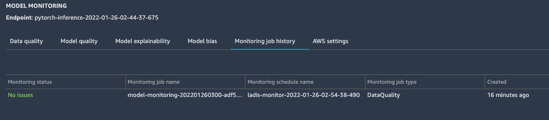
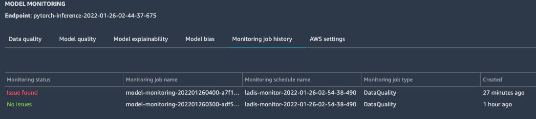
We can then check the Model Monitor display in Amazon SageMaker Studio or use Amazon CloudWatch logs to see if an issue was found.
Next, we use the adversarial inputs against the model hosted on SageMaker. We use the test dataset of the Tiny ImageNet dataset and apply the PGD attack, which introduces perturbations at the pixel level such that the model doesn’t recognize correct classes. In the following images, the left column shows two original test images, the middle column shows their adversarially perturbed versions, and the right column shows the difference between both images.
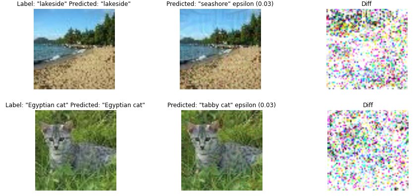
Now we can check the Model Monitor status and see that some of the inference images were drawn from a different distribution.
Results and user action
The custom Model Monitor job determines scores for each inference request, which indicates how likely the sample is adversarial according to the MMD test. These scores are gathered for all inference requests. Their score with the corresponding Debugger step number is recorded in a JSON file and uploaded to Amazon S3. After the Model Monitoring job is complete, we download the JSON file, retrieve step numbers, and use Debugger to retrieve the corresponding model inputs for these steps. This allows us to inspect the images that were detected as adversarial.
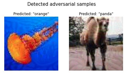
The following code block plots the first two images that have been identified as the most likely to be adversarial:
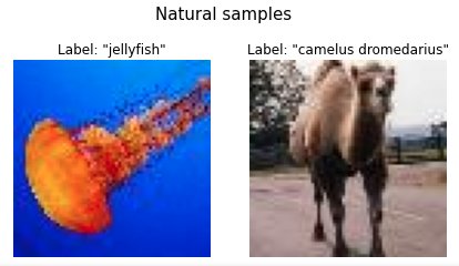
In our example test run, we get the following output. The jellyfish image was incorrectly predicted as an orange, and the camel image as a panda. Obviously, the model failed on these inputs and didn’t even predict a similar image class, such as goldfish or horse. For comparison, we also show the corresponding natural samples from the test set on the right side. We can observe that the random perturbations introduced by the attacker are very visible in the background of both images.
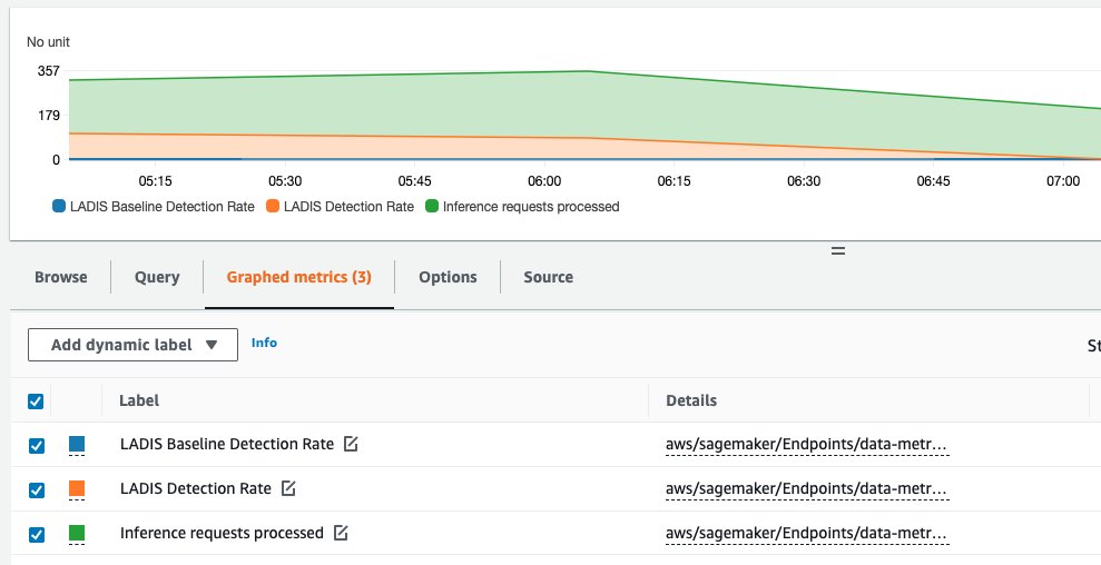
The custom Model Monitor job publishes the detection rate to CloudWatch, so we can investigate how this rate changed over time. A significant change between two data points may indicate that an adversary was trying to fool the model at a specific time frame. Additionally, you can also plot the number of inference requests being processed in each Model Monitor job and the baseline detection rate, which is computed over the validation dataset. The baseline rate is usually close to 0 and only serves as a comparison metric.
The following screenshot shows the metrics generated by our test runs, which ran three Model Monitoring jobs over 3 hours. Each job processes approximately 200–300 inference requests at a time. The detection rate is 100% between 5:00 PM and 6:00 PM, and drops afterwards.
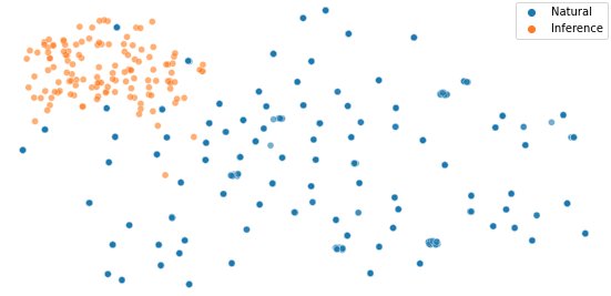
Furthermore, we can also inspect the distributions of representations generated by the intermediate layers of the model. With Debugger, we can access the data from the validation phase of the training job and the tensors from the inference phase, and use t-SNE to visualize their distribution for certain predicted classes. See the following code:
In our test case, we get the following t-SNE visualization for the second image class. We can observe that the adversarial samples are clustered differently than the natural ones.
Summary
In this post, we showed how to use a two-sample test using maximum mean discrepancy to detect adversarial inputs. We demonstrated how you can deploy such detection mechanisms using Debugger and Model Monitor. This workflow allows you to monitor your models hosted on SageMaker at scale and detect adversarial inputs automatically. To learn more about it, check out our GitHub repo.
References
[1] Aleksander Madry, Aleksandar Makelov, Ludwig Schmidt, Dimitris Tsipras, and Adrian Vladu. Towards deep learning models resistant to adversarial attacks. In International Conference on Learning Representations, 2018. [2] Laurens van der Maaten and Geoffrey Hinton. Visualizing data using t-SNE. Journal of Machine Learning Research, 9:2579–2605, 2008. URL http://www.jmlr.org/papers/v9/vandermaaten08a.html.About the Authors
 Nathalie Rauschmayr is a Senior Applied Scientist at AWS, where she helps customers develop deep learning applications.
 Yigitcan Kaya is a fifth year PhD student at University of Maryland and an applied scientist intern at AWS, working on security of machine learning and applications of machine learning for security.
 Bilal Zafar is an Applied Scientist at AWS, working on Fairness, Explainability and Security in Machine Learning.
 Sergul Aydore is a Senior Applied Scientist at AWS working on Privacy and Security in Machine Learning
 Rumi Olsen is a Solutions Architect in the AWS Partner Program. She specializes in serverless and machine learning solutions in her current role, and has a background in natural language processing technologies. She spends most of her spare time with her daughter exploring the nature of Pacific Northwest.


 Huong Nguyen is a Sr. Product Manager at AWS. She is leading the user experience for SageMaker Studio. She has 13 years’ experience creating customer-obsessed and data-driven products for both enterprise and consumer spaces. In her spare time, she enjoys reading, being in nature, and spending time with her family.