Posts in category: Amazon AWS

In this post, we present a solution for digitizing transactional documents using Amazon Textract and incorporate a human review using Amazon Augmented AI (A2I). You can find the solution source at our GitHub repository.

Organizations must frequently process scanned transactional documents with structured text so they can perform operations such as fraud detection or financial approvals. Some common examples of transactional documents that contain tabular data include bank statements, invoices, and bills of materials. Manually extracting data from such documents is expensive, time-consuming, and often requires a significant investment in training a specialized workforce. With the architecture outlined in this post, you can digitize tabular data from even low-quality scanned documents and achieve a high degree of accuracy.

Significant strides have been made with machine learning (ML)-based algorithms to increase accuracy and reliability when processing scanned text documents. These algorithms often match human-level performance in recognizing text and extracting content. Amazon Textract is a fully managed service that automatically extracts printed text, handwriting, and other data from scanned documents. Additionally, Amazon Textract can automatically identify and extract forms and tables from scanned documents.

Companies dealing with complex, varying, and sensitive documents often need human oversight to ensure accuracy, consistency, and compliance of the extracted data. As human reviewers provide input, you can fine-tune AI models to capture subtle nuances of a particular business process. Amazon A2I is an ML service that makes it easy to build the workflows required for human review. Amazon A2I removes the undifferentiated heavy lifting associated with building human review systems or managing a large number of human reviewers, and provides a unified and secure experience to your workforce.

Extracting transactional data from scanned documents, such as a list of debit card transactions on a bank statement, poses a unique set of challenges. Combining artificial intelligence with human review provides a practical approach to overcome these hurdles. An integrated solution that combines Amazon Textract and Amazon A2I is one such compelling example.

Consumers routinely use their smartphones to scan and upload transactional documents. Depending on the overall scan quality, including lighting conditions, skewed perspective, and less-than-adequate image resolution, it’s not uncommon to see suboptimal accuracy when these documents are processed using computer vision (CV) techniques. At the same time, handling scanned documents using manual labor can result in increased processing costs and processing time, and can limit your ability to scale up the volume of documents a pipeline can handle.

Solution overview

The following diagram illustrates the workflow of our solution:

Our end-to-end workflow performs the following steps:

1. Extracts tables from scanned source documents.
2. Applies custom business rules when extracting data from the tables.
3. Selectively escalates challenging documents for human review.
4. Performs postprocessing on the extracted data.
5. Stores the results.

A custom user interface built with ReactJS is provided to human reviewers to intuitively and efficiently review and correct issues in the documents when Amazon Textract provides a low-confidence extraction score, for example when text is obscured, fuzzy, or otherwise unclear.

Our reference solution uses a highly resilient pipeline, as detailed in the following diagram, to coordinate the various document processing stages.

The solution incorporates several architectural best practices:

• Batch processing – When possible, the solution should collect multiple documents and perform batch operations so we can optimize throughput and use resources more efficiently. For example, calling a custom AI model to run inference one time for a group of documents, as opposed to calling the model for each document individually. The design of our solution should enable batching when appropriate.
• Priority adjustment – When the volume of documents in the queue increases and the solution is no longer able to process them in a timely manner, we need a way to indicate that certain documents are higher priority, and therefore must be processed ahead of other documents in the queue.
• Auto scaling – The solution should be capable of scaling up and down dynamically. Many document processing workflows need to support the cyclical nature of demand. We should design the solution such that it can seamlessly scale up to handle spikes in load and scale back down when the load subsides.
• Self-regulation – The solution should be capable of gracefully handling external service outages and rate limitations.

Document processing stages

In this section, we walk you through the details of each stage in the document processing workflow:

• Acquisition
• Conversion
• Extraction
• Reshaping
• Custom business operations
• Augmentation
• Cataloging

Acquisition

The first stage of the pipeline acquires input documents from Amazon Simple Storage Service (Amazon S3). In this stage, we store initial document information in an Amazon DynamoDB table after receiving an S3 event notification via Amazon Simple Queue Service (Amazon SQS). We use this table record to track the progression of this document across the entire pipeline.

The order of priority for each document is determined by sorting the alphanumeric input key prefix in the document path. For example, a document stored with key acquire/p0/doc.pdf results in priority p0, and takes precedence over another document stored with key acquire/p1/doc.pdf (resulting in priority p1). Documents with no priority indicator in the key are processed at the end.

Conversion

Documents acquired from the previous stage are converted into PDF format, so we can provide a consistent data format for the rest of the pipeline. This allows us to batch multiple pages of a related document.

Extraction

PDF documents are sent to Amazon Textract to perform optical character recognition (OCR). Results from Amazon Textract are stored as JSON in a folder in Amazon S3.

Reshaping

Amazon Textract provides detailed information from the processed document, including raw text, key-value pairs, and tables. A significant amount of additional metadata identifies the location and relationship between the detected entity blocks. The transactional data is selected for further processing at this stage.

Custom business operations

Custom business rules are applied to the reshaped output containing information about tables in the document. Custom rules may include table format detection (such as detecting that a table contains checking transactions) or column validation (such as verifying that a product code column only contains valid codes).

Augmentation

Human annotators use Amazon A2I to review the document and augment it with any information that was missed. The review includes analyzing each table in the document for errors such as incorrect table types, field headers, and individual cell text that was incorrectly predicted. Confidence scores provided by the extraction stage are displayed in the UI to help human reviewers locate less accurate predictions easily. The following screenshot shows the custom UI used for this purpose.

Our solution uses a private human review workforce consisting of in-house annotators. This is an ideal option when dealing with sensitive documents or documents that require highly specialized domain knowledge. Amazon A2I also supports human review workforces through Amazon Mechanical Turk and Amazon’s authorized data labeling partners.

Cataloging

Documents that pass human review are cataloged into an Excel workbook so your business teams can easily consume them. The workbook contains each table detected and processed in the source document in their respective sheet, which is labeled with table type and page number. These Excel files are stored in a folder in Amazon S3 for consumption by business applications, for example, performing fraud detection using ML techniques.

Deploy the solution

This reference solution is available on GitHub, and you can deploy it with the AWS Cloud Development Kit (AWS CDK). The AWS CDK uses the familiarity and expressive power of programming languages for modeling your applications. It provides high-level components called constructs that preconfigure cloud resources with proven defaults, so you can build cloud applications with ease.

For instructions on deploying the cloud application, refer to the README file in the GitHub repo.

Solution demonstration

The following video walks you through a demonstration of the solution.

Conclusion

This post showed how you can build a custom digitization solution to process transactional documents with Amazon Textract and Amazon A2I. We automated and augmented input manifests, and enforced custom business rules. We also provided an intuitive user interface for human workforces to review data with low confidence scores, make necessary adjustments, and use feedback to improve the underlying ML models. The ability to use a custom frontend framework like ReactJS allows us to create modern web applications that serve our precise needs, especially when using public, private, or third-party data labeling workforces.

For more information about Amazon Textract and Amazon A2I, see Using Amazon Augmented AI to Add Human Review to Amazon Textract Output. For video presentations, sample Jupyter notebooks, or information about use cases like document processing, content moderation, sentiment analysis, text translation, and more, see Amazon Augmented AI Resources.

About the Team

The Amazon ML Solutions Lab pairs your organization with ML experts to help you identify and build ML solutions to address your organization’s highest return-on-investment ML opportunities. Through discovery workshops and ideation sessions, the ML Solutions Lab “works backward” from your business problems to deliver a roadmap of prioritized ML use cases with an implementation plan to address them. Our ML scientists design and develop advanced ML models in areas such as computer vision, speech processing, and natural language processing to solve customers’ problems, including solutions requiring human review.

About the Authors

Pri Nonis is a Deep Learning Architect at the Amazon ML Solutions Lab, where he works with customers across various verticals, and helps them accelerate their cloud migration journey, and to solve their ML problems using state-of-the-art solutions and technologies.

Dan Noble is a Software Development Engineer at Amazon where he helps build delightful user experiences. In his spare time, he enjoys reading, exercising, and having adventures with his family.

Jae Sung Jang is a Software Development Engineer. His passion lies with automating manual process using AI Solutions and Orchestration technologies to ensure business execution.

Jeremy Feltracco is a Software Development Engineer with the Amazon ML Solutions Lab at Amazon Web Services. He uses his background in computer vision, robotics, and machine learning to help AWS customers accelerate their AI adoption.

David Dasari is a manager at the Amazon ML Solutions Lab, where he helps AWS customers accelerate their AI and cloud adoption in the Human-In-The-Loop solutions across various industry verticals. With ERP and payment services as his background, was obsessed towards ML/AI taking strides in delighting customers that drove him to this field.

Read More

Data lakes have become the norm in the industry for storing critical business data. The primary rationale for a data lake is to land all types of data, from raw data to preprocessed and postprocessed data, and may include both structured and unstructured data formats. Having a centralized data store for all types of data allows modern big data applications to load, transform, and process whatever type of data is needed. Benefits include storing data as is without the need to first structure or transform it. Most importantly, data lakes allow controlled access to data from many different types of analytics and machine learning (ML) processes in order to guide better decision-making.

Multiple vendors have created data lake architectures, including AWS Lake Formation. In addition, open-source solutions allow companies to access, load, and share data easily. One of the options for storing data in the AWS Cloud is Delta Lake. The Delta Lake library enables reads and writes in open-source Apache Parquet file format, and provides capabilities like ACID transactions, scalable metadata handling, and unified streaming and batch data processing. Delta Lake offers a storage layer API that you can use to store data on top of an object-layer storage like Amazon Simple Storage Service (Amazon S3).

Data is at the heart of ML—training a traditional supervised model is impossible without access to high-quality historical data, which is commonly stored in a data lake. Amazon SageMaker is a fully managed service that provides a versatile workbench for building ML solutions and provides highly tailored tooling for data ingestion, data processing, model training, and model hosting. Apache Spark is a workhorse of modern data processing with an extensive API for loading and manipulating data. SageMaker has the ability to prepare data at petabyte scale using Spark to enable ML workflows that run in a highly distributed manner. This post highlights how you can take advantage of the capabilities offered by Delta Lake using Amazon SageMaker Studio.

Solution overview

In this post, we describe how to use SageMaker Studio notebooks to easily load and transform data stored in the Delta Lake format. We use a standard Jupyter notebook to run Apache Spark commands that read and write table data in CSV and Parquet format. The open-source library delta-spark allows you to directly access this data in its native format. This library allows you to take advantage of the many API operations to apply data transformations, make schema modifications, and use time-travel or as-of-timestamp queries to pull a particular version of the data.

In our sample notebook, we load raw data into a Spark DataFrame, create a Delta table, query it, display audit history, demonstrate schema evolution, and show various methods for updating the table data. We use the DataFrame API from the PySpark library to ingest and transform the dataset attributes. We use the delta-spark library to read and write data in Delta Lake format and to manipulate the underlying table structure, referred to as the schema.

We use SageMaker Studio, the built-in IDE from SageMaker, to create and run Python code from a Jupyter notebook. We have created a GitHub repository that contains this notebook and other resources to run this sample on your own. The notebook demonstrates exactly how to interact with data stored in Delta Lake format, which permits tables to be accessed in-place without the need to replicate data across disparate datastores.

For this example, we use a publicly available dataset from Lending Club that represents customer loans data. We downloaded the accepted data file (accepted_2007_to_2018Q4.csv.gz), and selected a subset of the original attributes. This dataset is available under the Creative Commons (CCO) License.

Prerequisites

You must install a few prerequisites prior to using the delta-spark functionality. To satisfy required dependencies, we have to install some libraries into our Studio environment, which runs as a Dockerized container and is accessed via a Jupyter Gateway app:

• OpenJDK for access to Java and associated libraries
• PySpark (Spark for Python) library
• Delta Spark open-source library

We can use either conda or pip to install these libraries, which are publicly available in either conda-forge, PyPI servers, or Maven repositories.

This notebook is designed to run within SageMaker Studio. After you launch the notebook within Studio, make sure you choose the Python 3(Data Science) kernel type. Additionally, we suggest using an instance type with at least 16 GB of RAM (like ml.g4dn.xlarge), which allows PySpark commands to run faster. Use the following commands to install the required dependencies, which make up the first several cells of the notebook:

%conda install openjdk -q -y
%pip install pyspark==3.2.0
%pip install delta-spark==1.1.0
%pip install -U "sagemaker>2.72"

After the installation commands are complete, we’re ready to run the core logic in the notebook.

Implement the solution

To run Apache Spark commands, we need to instantiate a SparkSession object. After we include the necessary import commands, we configure the SparkSession by setting some additional configuration parameters. The parameter with key spark.jars.packages passes the names of additional libraries used by Spark to run delta commands. The following initial lines of code assemble a list of packages, using traditional Maven coordinates (groupId:artifactId:version), to pass these additional packages to the SparkSession.

Additionally, the parameters with key spark.sql.extensions and spark.sql.catalog.spark_catalog enable Spark to properly handle Delta Lake functionality. The final configuration parameter with key fs.s3a.aws.credentials.provider adds the ContainerCredentialsProvider class, which allows Studio to look up the AWS Identity and Access Management (IAM) role permissions made available via the container environment. The code creates a SparkSession object that is properly initialized for the SageMaker Studio environment:

# Configure Spark to use additional library packages to satisfy dependencies

# Build list of packages entries using Maven coordinates (groupId:artifactId:version)
pkg_list = []
pkg_list.append("io.delta:delta-core_2.12:1.1.0")
pkg_list.append("org.apache.hadoop:hadoop-aws:3.2.2")

packages=(",".join(pkg_list))
print('packages: '+packages)

# Instantiate Spark via builder
# Note: we use the `ContainerCredentialsProvider` to give us access to underlying IAM role permissions

spark = (SparkSession
    .builder
    .appName("PySparkApp") 
    .config("spark.jars.packages", packages) 
    .config("spark.sql.extensions", "io.delta.sql.DeltaSparkSessionExtension") 
    .config("spark.sql.catalog.spark_catalog", "org.apache.spark.sql.delta.catalog.DeltaCatalog") 
    .config("fs.s3a.aws.credentials.provider", 
"com.amazonaws.auth.ContainerCredentialsProvider") 
    .getOrCreate()) 

sc = spark.sparkContext

print('Spark version: '+str(sc.version))

In the next section, we upload a file containing a subset of the Lending Club consumer loans dataset to our default S3 bucket. The original dataset is very large (over 600 MB), so we provide a single representative file (2.6 MB) for use by this notebook. PySpark uses the s3a protocol to enable additional Hadoop library functionality. Therefore, we modify each native S3 URI from the s3 protocol to use s3a in the cells throughout this notebook.

We use Spark to read in the raw data (with options for both CSV or Parquet files) with the following code, which returns a Spark DataFrame named loans_df:

loans_df = spark.read.csv(s3a_raw_csv, header=True)

The following screenshot shows the first 10 rows from the resulting DataFrame.

We can now write out this DataFrame as a Delta Lake table with a single line of code by specifying .format("delta") and providing the S3 URI location where we want to write the table data:

loans_df.write.format("delta").mode("overwrite").save(s3a_delta_table_uri)

The next few notebook cells show an option for querying the Delta Lake table. We can construct a standard SQL query, specify delta format and the table location, and submit this command using Spark SQL syntax:

sql_cmd = f'SELECT * FROM delta.`{s3a_delta_table_uri}` ORDER BY loan_amnt'
sql_results = spark.sql(sql_cmd)

The following screenshot shows the results of our SQL query as ordered by loan_amnt.

Interact with Delta Lake tables

In this section, we showcase the DeltaTable class from the delta-spark library. DeltaTable is the primary class for programmatically interacting with Delta Lake tables. This class includes several static methods for discovering information about a table. For example, the isDeltaTable method returns a Boolean value indicating whether the table is stored in delta format:

# Use static method to determine table type
print(DeltaTable.isDeltaTable(spark, s3a_delta_table_uri))

You can create DeltaTable instances using the path of the Delta table, which in our case is the S3 URI location. In the following code, we retrieve the complete history of table modifications:

deltaTable = DeltaTable.forPath(spark, s3a_delta_table_uri)
history_df = deltaTable.history()
history_df.head(3)

The output indicates the table has six modifications stored in the history, and shows the latest three versions.

Schema evolution

In this section, we demonstrate how Delta Lake schema evolution works. By default, delta-spark forces table writes to abide by the existing schema by enforcing constraints. However, by specifying certain options, we can safely modify the schema of the table.

First, let’s read data back in from the Delta table. Because this data was written out as delta format, we need to specify .format("delta") when reading the data, then we provide the S3 URI where the Delta table is located. Second, we write the DataFrame back out to a different S3 location where we demonstrate schema evolution. See the following code:

delta_df = (spark.read.format("delta").load(s3a_delta_table_uri))
delta_df.write.format("delta").mode("overwrite").save(s3a_delta_update_uri)

Now we use the Spark DataFrame API to add two new columns to our dataset. The column names are funding_type and excess_int_rate, and the column values are set to constants using the DataFrame withColumn method. See the following code:

funding_type_col = "funding_type"
excess_int_rate_col = "excess_int_rate"

delta_update_df = (delta_df.withColumn(funding_type_col, lit("NA"))
                           .withColumn(excess_int_rate_col, lit(0.0)))
delta_update_df.dtypes

A quick look at the data types (dtypes) shows the additional columns are part of the DataFrame.

Now we enable the schema modification, thereby changing the underlying schema of the Delta table, by setting the mergeSchema option to true in the following Spark write command:

(delta_update_df.write.format("delta")
 .mode("overwrite")
 .option("mergeSchema", "true") # option - evolve schema
 .save(s3a_delta_update_uri)
)

Let’s check the modification history of our new table, which shows that the table schema has been modified:

deltaTableUpdate = DeltaTable.forPath(spark, s3a_delta_update_uri)

# Let's retrieve history BEFORE schema modification
history_update_df = deltaTableUpdate.history()
history_update_df.show(3)

The history listing shows each revision to the metadata.

Conditional table updates

You can use the DeltaTable update method to run a predicate and then apply a transform whenever the condition evaluates to True. In our case, we write the value FullyFunded to the funding_type column whenever the loan_amnt equals the funded_amnt. This is a powerful mechanism for writing conditional updates to your table data.

deltaTableUpdate.update(condition = col("loan_amnt") == col("funded_amnt"),
    set = { funding_type_col: lit("FullyFunded") } )

The following screenshot shows our results.

In the final change to the table data, we show the syntax to pass a function to the update method, which in our case calculates the excess interest rate by subtracting 10.0% from the loan’s int_rate attribute. One more SQL command pulls records that meet our condition, using the WHERE clause to locate records with int_rate greater than 10.0%:

# Function that calculates rate overage (amount over 10.0)
def excess_int_rate(rate):
    return (rate-10.0)

deltaTableUpdate.update(condition = col("int_rate") > 10.0,
 set = { excess_int_rate_col: excess_int_rate(col("int_rate")) } )

The new excess_int_rate column now correctly contains the int_rate minus 10.0%.

Our last notebook cell retrieves the history from the Delta table again, this time showing the modifications after the schema modification has been performed:

# Finally, let's retrieve table history AFTER the schema modifications

history_update_df = deltaTableUpdate.history()
history_update_df.show(3)

The following screenshot shows our results.

Conclusion

You can use SageMaker Studio notebooks to interact directly with data stored in the open-source Delta Lake format. In this post, we provided sample code that reads and writes this data using the open source delta-spark library, which allows you to create, update, and manage the dataset as a Delta table. We also demonstrated the power of combining these critical technologies to extract value from preexisting data lakes, and showed how to use the capabilities of Delta Lake on SageMaker.

Our notebook sample provides an end-to-end recipe for installing prerequisites, instantiating Spark data structures, reading and writing DataFrames in Delta Lake format, and using functionalities like schema evolution. You can integrate these technologies to magnify their power to provide transformative business outcomes.

About the Authors

Paul Hargis has focused his efforts on Machine Learning at several companies, including AWS, Amazon, and Hortonworks. He enjoys building technology solutions and also teaching people how to make the most of it. Prior to his role at AWS, he was lead architect for Amazon Exports and Expansions helping amazon.com improve experience for international shoppers. Paul likes to help customers expand their machine learning initiatives to solve real-world problems.

Vedant Jain is a Sr. AI/ML Specialist Solutions Architect, helping customers derive value out of the Machine Learning ecosystem at AWS. Prior to joining AWS, Vedant has held ML/Data Science Specialty positions at various companies such as Databricks, Hortonworks (now Cloudera) & JP Morgan Chase. Outside of his work, Vedant is passionate about making music, using Science to lead a meaningful life & exploring delicious vegetarian cuisine from around the world.

Read More

Amazon Comprehend is a natural language processing (NLP) service that uses machine learning (ML) to discover insights from text. As a fully managed service, Amazon Comprehend requires no ML expertise and can scale to large volumes of data. Amazon Comprehend provides several different APIs to easily integrate NLP into your applications. You can simply call the APIs in your application and provide the location of the source document or text. The APIs output entities, key phrases, sentiment, document classification, and language in an easy-to-use format for your application or business.

The sentiment analysis APIs provided by Amazon Comprehend help businesses determine the sentiment of a document. You can gauge the overall sentiment of a document as positive, negative, neutral, or mixed. However, to get the granularity of understanding the sentiment associated with specific products or brands, businesses have had to employ workarounds like chunking the text into logical blocks and inferring the sentiment expressed towards a specific product.

To help simplify this process, starting today, Amazon Comprehend is launching the Targeted Sentiment feature for sentiment analysis. This provides the capability to identify groups of mentions (co-reference groups) corresponding to a single real-world entity or attribute, provide the sentiment associated with each entity mention, and provide the classification of the real-world entity based on a pre-determined list of entities.

This post provides an overview of how you can get started with Amazon Comprehend targeted sentiment, demonstrates what you can do with the output, and walks through three common targeted sentiment use cases.

Solution overview

The following is an example of targeted sentiment:

“Spa” is the primary entity, identified as type facility, and is mentioned two more times, referred to as the pronoun “it.” The Targeted Sentiment API provides the sentiment towards each entity. Positive sentiment is green, negative is red,  and neutral is blue. We can also determine how the sentiment towards the spa changes throughout the sentence. We dive deeper into the API later in the post.

This capability opens up several different capabilities for businesses. Marketing teams can track popular sentiments toward their brands in social media over time. Ecommerce merchants can understand which specific attributes of their products were best- and worst-received by customers. Call center operators can use the feature to mine transcripts for escalation issues and to monitor customer experience. Restaurants, hotels, and other hospitality industry organizations can use the service to turn broad ratings categories into rich descriptions of good and bad customer experiences.

Targeted sentiment use cases

The Targeted Sentiment API in Amazon Comprehend takes text data such as social media posts, application reviews, and call center transcriptions as input. Then it analyzes the input using the power of NLP algorithms to extract entity-level sentiment automatically. An entity is a textual reference to the unique name of a real-world object, such as people, places, and commercial items, in addition to precise references to measures such as dates and quantities. For a full list of supported entities, refer to Targeted Sentiment Entities.

We use the Targeted Sentiment API to enable the following use cases:

• A business can identify parts of the employee/customer experience that are enjoyable and parts that may be improved.
• Contact centers and customer service teams can analyze on-call transcriptions or chat logs to identify agent training effectiveness, and conversation details such as specific reactions from a customer and phrases or words that were used to illicit that response.
• Product owners and UI/UX developers can identify features of their product that users enjoy and parts that require improvement. This can support product roadmap discussions and prioritizations.

The following diagram illustrates the targeted sentiment process:

In this post, we demonstrate this process using the following three sample reviews:

• Sample 1: Business and product review – “I really like how thick the jacket is. I wear a large jacket because I have broad shoulders and that’s what I ordered and it fits perfectly there. I almost feel like it balloons out from the chest down. I thought I would use the strings in the bottom of the jacket to help close it and bring it in, but those don’t work. The jacket feels very bulky.”
• Sample 2: Contact center transcription – “Hi there, there is a fraud block on my credit card, can you remove it for me. My credit card keeps getting flagged for fraud. It is quite annoying, every time I go to use it, I keep getting declined. I’m going to cancel the card if this happens again.”
• Sample 3: Employer feedback survey – “I’m glad management is upskilling the team. But the instructor did not go over the basics well. Management should do more due diligence on everyone’s skill level for future sessions.”

Prepare the data

To get started, download the sample files containing the example text using the AWS Command Line Interface (AWS CLI) by running the following commands:

aws s3 cp s3://aws-blogs-artifacts-public/artifacts/ML-8148/ts-sample-data.zip .

Create an Amazon Simple Storage Service (Amazon S3) bucket, unzip the folder and upload the folder containing the three sample files. Make sure you’re using the same Region throughout.

You can now access the three sample text files in your S3 bucket.

Create a job in Amazon Comprehend

After you upload the files to your S3 bucket, complete the following steps:

1. On the Amazon Comprehend console, choose Analysis jobs in the navigation pane.
   
2. Choose Create job.
   
3. For Name, enter a name for your job.
4. For Analysis type, choose Targeted sentiment.
5. Under Input data, enter the Amazon S3 location of the ts-sample-data folder.
6. For Input format, choose One document per file.

You can change this configuration if your data is in a single file delimited by lines.

7. Under Output location, enter the Amazon S3 location where you want to save the job output.
8. Under Access permissions, for IAM role, choose an existing AWS Identity and Access Management (IAM) role or create one that has permissions to the S3 bucket.
9. Leave the other options as default and choose Create job.
   

After you start the job, you can review your job details. The total job runtime depends on the size of the input data.

10. When the job is complete, under Output, choose the link to the output data location.
    

Here you can find a compressed output file.

11. Download and decompress the file.

You can now inspect the output files for each sample text. Open the files in your preferred text editor to review the API response structure. We describe this in more detail in the next section.

API response structure

The Targeted Sentiment API provides a simple way to consume the output of your jobs. It provides a logical grouping of the entities (entity groups) detected, along with the sentiment for each entity. The following are some definitions of the fields that are in the response:

• Entities – The significant parts of the document. For example, Person, Place, Date, Food, or Taste.
• Mentions – The references or mentions of the entity in the document. These can be pronouns or common nouns such as “it,” “him,” “book,” and so on. These are organized in order by location (offset) in the document.
• DescriptiveMentionIndex – The index in Mentions that gives the best depiction of the entity group. For example, “ABC Hotel” instead of “hotel,” “it,” or other common noun mentions.
• GroupScore – The confidence that all the entities mentioned in the group are related to the same entity (such as “I,” “me,” and “myself” referring to one person).
• Text – The text in the document that depicts the entity
• Type – A description of what the entity depicts.
• Score – The model confidence that this is a relevant entity.
• MentionSentiment – The actual sentiment found for the mention.
• Sentiment – The string value of positive, neutral, negative, or mixed.
• SentimentScore – The model confidence for each possible sentiment.
• BeginOffset – The offset into the document text where the mention begins.
• EndOffset – The offset into the document text where the mention ends.

To demonstrate this visually, let’s take the output of the third use case, the employer feedback survey, and walk through the entity groups that represent the employee completing the survey, management, and the instructor.

Let’s first look at all the mentions of the co-reference entity group associated with “I” (the employee writing the response) and the location of the mention in the text. DescriptiveMentionIndex represents indexes of the entity mentions that best depict the co-reference entity group (in this case I):

{
      "DescriptiveMentionIndex": [
        0
      ],
      "Mentions": [
        {
          "BeginOffset": 0,
          "EndOffset": 1,
          "Score": 0.999997,
          "GroupScore": 1,
          "Text": "I",
          "Type": "PERSON",
          "MentionSentiment": {
            "Sentiment": "NEUTRAL",
            "SentimentScore": {
              "Mixed": 0,
              "Negative": 0,
              "Neutral": 1,
              "Positive": 0
            }
          }
        }
      ]
    }

The next group of entities provides all mentions of the co-reference entity group associated with management, along with its location in the text. DescriptiveMentionIndex represents indexes of the entity mentions that best depict the co-reference entity group (in this case management). Something to observe in this example is the sentiment shift towards management. You can use this data to infer what parts of management’s actions were perceived as positive, and what parts were perceived as negative and therefore can be improved upon.

{
      "DescriptiveMentionIndex": [
        0,
        1
      ],
      "Mentions": [
        {
          "BeginOffset": 9,
          "EndOffset": 19,
          "Score": 0.999984,
          "GroupScore": 1,
          "Text": "management",
          "Type": "ORGANIZATION",
          "MentionSentiment": {
            "Sentiment": "POSITIVE",
            "SentimentScore": {
              "Mixed": 0,
              "Negative": 0,
              "Neutral": 0,
              "Positive": 1
            }
          }
        },
        {
          "BeginOffset": 103,
          "EndOffset": 113,
          "Score": 0.999998,
          "GroupScore": 0.999896,
          "Text": "Management",
          "Type": "ORGANIZATION",
          "MentionSentiment": {
            "Sentiment": "NEGATIVE",
            "SentimentScore": {
              "Mixed": 0.000149,
              "Negative": 0.990075,
              "Neutral": 0.000001,
              "Positive": 0.009775
            }
          }
        }
      ]
    }

To conclude, let’s observe all mentions of the instructor and the location in the text. DescriptiveMentionIndex represents indexes of the entity mentions that best depict the co-reference entity group (in this case instructor):

{
      "DescriptiveMentionIndex": [
        0
      ],
      "Mentions": [
        {
          "BeginOffset": 52,
          "EndOffset": 62,
          "Score": 0.999996,
          "GroupScore": 1,
          "Text": "instructor",
          "Type": "PERSON",
          "MentionSentiment": {
            "Sentiment": "NEGATIVE",
            "SentimentScore": {
              "Mixed": 0,
              "Negative": 0.999997,
              "Neutral": 0.000001,
              "Positive": 0.000001
            }
          }
        }
      ]
    }

Reference architecture

You can apply targeted sentiment to many scenarios and use cases to drive business value, such as the following:

• Determine efficacy of marketing campaigns and feature launches by detecting the entities and mentions that contain the most positive or negative feedback
• Query output to determine which entities and mentions relate to a corresponding entity (positive, negative, or neutral)
• Analyze sentiment across the customer interaction lifecycle in contact centers to demonstrate efficacy of process or training changes

The following diagram depicts an end-to-end process:

Conclusion

Understanding the interactions and feedback organizations receive from customers about their products and services remains crucial in developing better products and customer experiences. As such, more granular details are required to infer better outcomes.

In this post, we provided some examples of how using these granular details can help organizations improve products, customer experiences, and training while also incentivizing and validating positive attributes. There are many use cases across industries where you can experiment with and gain value from targeted sentiment.

We encourage you to try this new feature with your use cases. For more information and to get started, refer to Targeted Sentiment.

About the Authors

Raj Pathak is a Solutions Architect and Technical advisor to Fortune 50 and Mid-Sized FSI (Banking, Insurance, Capital Markets) customers across Canada and the United States. Raj specializes in Machine Learning with applications in Document Extraction, Contact Center Transformation and Computer Vision.

Sanjeev Pulapaka is a Senior Solutions Architect in the U.S. Fed Civilian SA team at Amazon Web Services (AWS). He works closely with customers in building and architecting mission critical solutions. Sanjeev has extensive experience in leading, architecting and implementing high-impact technology solutions that address diverse business needs in multiple sectors including commercial, federal, state and local governments. He has an undergraduate degree in engineering from the Indian Institute of Technology and an MBA from the University of Notre Dame.

Read More

Amazon SageMaker Autopilot automatically builds, trains, and tunes the best machine learning (ML) models based on your data, while allowing you to maintain full control and visibility. We have recently announced support for time series data in Autopilot. You can use Autopilot to tackle regression and classification tasks on time series data, or sequence data in general. Time series data is a special type of sequence data where data points are collected at even time intervals.

Manually preparing the data, selecting the right ML model, and optimizing its parameters is a complex task, even for an expert practitioner. Although automated approaches exist that can find the best models and their parameters, these typically can’t handle data that comes as sequences, such as network traffic, electricity consumption, or household expenses recorded over time. Because this data takes the form of observations acquired at different time points, consecutive observations can’t be treated as independent of each other and need to be processed as a whole. You can use Autopilot for a wide range of problems dealing with sequential data. For example, you can classify network traffic recorded over time to identify malicious activities, or determine if individuals qualify for a mortgage based on their credit history. You provide a dataset containing time series data and Autopilot handles the rest, processing the sequential data through specialized feature transforms and finding the best model on your behalf.

Autopilot eliminates the heavy lifting of building ML models, and helps you automatically build, train, and tune the best ML model based on your data. Autopilot runs several algorithms on your data and tunes their hyperparameters on a fully managed compute infrastructure. In this post, we demonstrate how you can use Autopilot to solve classification and regression problems on time series data. For instructions on creating and training an Autopilot model, see Customer Churn Prediction with Amazon SageMaker Autopilot.

Time series data classification using Autopilot

As a running example, we consider a multi-class problem on the time series dataset UWaveGestureLibraryX, containing equidistant readings of accelerometer sensors while performing one of eight predefined hand gestures. For simplicity, we consider only X dimension of the accelerometer. The task is to build a classification model to map the time series data from the sensor readings to the predefined gestures. The following figure shows the first rows of the dataset in CSV format. The entire table consists of 896 rows and two columns: the first column is a gesture label and the second column is a time series of sensor readings.

Convert data to the right format with Amazon SageMaker Data Wrangler

On top of accepting numerical, categorical, and standard text columns, Autopilot now also accepts a sequence input column. If your time series data doesn’t follow this format, you can easily convert it through Amazon SageMaker Data Wrangler. Data Wrangler reduces the time it takes to aggregate and prepare data for ML from weeks to minutes. With Data Wrangler, you can simplify the process of data preparation and feature engineering, and complete each step of the data preparation workflow, including data selection, cleansing, exploration, and visualization from a single visual interface. For instance, consider the same dataset but in a different input format: each gesture (specified by ID) is a sequence of equidistant measurements of the accelerometer. When stored vertically, each row contains a timestamp and one value. The following figure compares this data in its original format and a sequence format.

To convert this dataset to the format described earlier using Data Wrangler, load the dataset from Amazon Simple Storage Service (Amazon S3). Then use the time series Group by transform, as shown in the following screenshot, and export the data back to Amazon S3 in CSV format.

When the dataset is in its designated format, you can proceed with Autopilot. To check out other time series transformers of Data Wrangler refer to Prepare time series data with Amazon SageMaker Data Wrangler.

Launch an AutoML job

As with other input types supported by Autopilot, each row of the dataset is a different observation and each column is a feature. In this example, we have a single column containing time series data, but you can have multiple time series columns. You can also have multiple columns with different input types, such as time series, text, and numerical.

To create an Autopilot experiment, place the dataset in an S3 bucket and create a new experiment within Amazon SageMaker Studio. As shown in the following screenshot, you must specify the name of experiment, S3 location of the dataset, S3 location for the output artifacts, and the column name to predict.

Autopilot analyzes the data, generates ML pipelines, and runs a default 250 iterations of hyperparameter optimization on this classification task. As shown in the following model leaderboard, Autopilot reaches 0.821 accuracy, and you can deploy the best model in just one click.

In addition, Autopilot generates a data exploration report, where you can visualize and explore your data.

Transparency is foundational for Autopilot. You can inspect and modify generated ML pipelines within the candidate definition notebook. The following screenshot demonstrates how Autopilot recommends a range of pipelines, combining the time series transformer TSFeatureExtractor with different ML algorithms, such as gradient boosted decision trees and linear models. The TSFeatureExtractor extracts hundreds of time series features for you, which are then fed to the downstream algorithms to make predictions. For the full list of time series features, refer to Overview on extracted features.

Conclusion

In this post, we demonstrated how to use SageMaker Autopilot to solve time series classification and regression problems in just a few clicks.

For more information about Autopilot, see Amazon SageMaker Autopilot. To explore related features of SageMaker, see Amazon SageMaker Data Wrangler.

About the Authors

Nikita Ivkin is an Applied Scientist, Amazon SageMaker Data Wrangler.

Anne Milbert is a Software Development engineer working on Amazon SageMaker Automatic Model Tuning.

Valerio Perrone is an Applied Science Manager working on Amazon SageMaker Automatic Model Tuning and Autopilot.

Meghana Satish is a Software Development engineer working on Amazon SageMaker Automatic Model Tuning.

Ali Takbiri is an AI/ML specialist Solutions Architect, and helps customers by using Machine Learning to solve their business challenges on the AWS Cloud.

Read More

With an Amazon SageMaker Domain, you can onboard users with an AWS Identity and Access Management (IAM) execution role different than the Domain execution role. In such case, the onboarded Domain user can’t create projects using templates and Amazon SageMaker JumpStart solutions. This post outlines an automated approach to enable JumpStart for Domain users with a custom execution role. We walk you through two different use cases for enabling JumpStart and how to solve these cases programmatically. The automated solution can help you scale your process to enable JumpStart for Domain users with custom roles, increasing productivity of your data science team and Amazon SageMaker Studio administrators.

JumpStart is a feature within Studio that helps you quickly and easily get started with machine learning (ML). With more and more customers increasingly using ML and adopting Amazon SageMaker, JumpStart is making it easier for data science and ML teams to access and fine-tune more than 150 popular open-source models, such as natural language processing, object detection, and image classification models.

Solution overview

JumpStart requires a SageMaker Domain with project templates enabled for the account and Studio users, as shown in the following screenshot.

If enabled, this setting allows users (configured to use the Domain execution role) to create projects using templates and JumpStart solutions. In the scenario where the user’s execution role is different than the Domain execution role, JumpStart remains disabled for that user even when it’s enabled on the Domain. We address this custom role scenario and the automated solution in the following sections.

In this solution, we address the issue for the following two cases:

• Use case 1 – Enabling JumpStart in an automated manner for existing Domain users with custom roles regardless of apps assigned
• Use case 2 – Providing a reference script that you can use to programmatically enable JumpStart while onboarding a new Domain user with a custom role

Domain user onboarding

After you create a Domain, you can onboard users to launch apps (such as Studio, RStudio, or Canvas). You must assign a default execution role to a Domain user during the creation process, as shown in the following screenshot.

You can choose a role different than the Domain execution role for a user. However, this may disable JumpStart for such users even when it’s enabled on the Domain. This behavior is due to the fact that SageMaker makes no assumption on a custom role and its permission boundary. The required permissions and policies have to be assigned explicitly to access templates and JumpStart solutions published by SageMaker in AWS Service Catalog.

You can enable SageMaker Projects and JumpStart manually for every user by selecting the user profile on the SageMaker Domain control panel. However, this process can be time-consuming if a user already has some apps assigned. The Edit button at bottom right is only enabled when no apps are assigned to that user (see the following screenshot). You have to delete the assigned apps first in order to edit a user profile.

The cause of the disabled JumpStart feature is evident during Step 2 of editing a user profile, where a message states “If there are individual users using custom execution roles in your organization, you need to enable them on the user profile page.”

In the following sections, we walk you through two automated solutions that cover use cases for both existing and new Domain users.

Prerequisites

The steps described as part of this solution have the following prerequisites:

• You have created a SageMaker Domain
• The SageMaker Domain authentication method is IAM
• Custom roles assigned to the SageMaker Domain users have the AmazonSageMakerFullAccess policy attached

In order for JumpStart Solutions to be enabled for users, the AWS Service Catalog portfolio Amazon SageMaker Solutions and ML Ops products must be imported into the account, and this portfolio must be associated with the role that runs SageMaker. The role association is necessary so that Studio can invoke AWS Service Catalog APIs associated with the Solutions portfolio.

As a general best practice, we recommend testing the process in a non-production environment followed by validation tests to make sure everything is configured and operating as per your expectations before making changes to the production environment.

Use case 1: Enable JumpStart for all existing Domain users with a custom role

Let’s first consider the use case for existing users and enable JumpStart for those users in an automated way.

To achieve this, we have created an AWS CloudFormation template that you can run in the same Region where the SageMaker Domain exists.

The CloudFormation stack contained in the attached jumpstart_solutions_resources.template.yaml file has the following components:

• AmazonSageMakerServiceCatalogProductsLaunchRole and AmazonSageMakerServiceCatalogProductsUseRole – Creates these two IAM roles, if they don’t already exist.
• 1PProductUseRolePolicy – Creates this policy used by AmazonSageMakerServiceCatalogProductsUseRole, if this role doesn’t already exist.
• setup_solutions_tests_portfolio – An AWS Lambda function that performs the AWS Service Catalog portfolio import and role association by calling Boto3 APIs. This function is called once during CloudFormation stack creation.
• LambdaIAMRole role – Used by the function setup_solutions_tests_portfolio for calling AWS Service Catalog and SageMaker APIs.
• SetupPortfolioInvoker – Invokes the function setup_solutions_tests_portfolio.

After the Lambda function runs as part of the CloudFormation deployment, it retrofits all the existing SageMaker Domain users to enable JumpStart and Projects for them. For more information on creating and monitoring a CloudFormation stack, refer to How does AWS CloudFormation work.

Use case 2: Enable JumpStart for a single Domain user with a custom role

Many customers prefer to scale the Domain user onboarding process by automating it programmatically. In this section, we provide a Python script reference that you can use as part of the onboarding process to enable JumpStart for a new user with a custom role. This Python script performs the required association for the given user role. The automated process calling this script must have permission to use AWS Service Catalog and SageMaker APIs. See the following code:

sagemaker_client = boto3.client("sagemaker")
sc_client = boto3.client("servicecatalog")

# function to return 'Amazon SageMaker' portfolio id
def get_solutions_portfolio_id(sc_client):
    portfolio_shares = sc_client.list_accepted_portfolio_shares()
    for portfolio in portfolio_shares['PortfolioDetails']:
            if portfolio['ProviderName'] == 'Amazon SageMaker':
                    return(portfolio['Id'])

portfolio_id = get_solutions_portfolio_id(sc_client)
# import Solutions Service Catalog Portfolio 
sagemaker_client.enable_sagemaker_servicecatalog_portfolio()
    	
sc_client.associate_principal_with_portfolio(
                    PortfolioId=portfolio_id,
                    PrincipalARN=, # custom role ARN
                    PrincipalType='IAM'
                    )

You can either call the script independently or embed it as a step within an automated process to create a user profile for onboarding to Studio. For more information on using Boto3, refer to Boto3 reference.

Clean up

After all the custom roles are enabled to use JumpStart, we can clean up the resources no longer needed. You can delete the Lambda function setup_solutions_tests_portfolio and the IAM role LambdaIAMRole created by the CloudFormation template. The other two IAM roles, AmazonSageMakerServiceCatalogProductsLaunchRole and AmazonSageMakerServiceCatalogProductsUseRole, and the associated policy 1PProductUseRolePolicy (if created) must not be deleted because they need to exist for accessing JumpStart.

Conclusion

In this post, we shared the steps to enable JumpStart for a custom role for existing users as well as new users programmatically. As always, make sure to validate the steps mentioned in this solution in a non-production environment before deploying to production.

Try it out and let us know if you have any questions in the comments section!

Additional resources

For more information, see the following:

• Amazon SageMaker resources
• Automate a centralized deployment of Amazon SageMaker Studio with AWS Service Catalog
• Configuring Amazon SageMaker Studio for teams and groups with complete resource isolation

About the Authors

Nikhil Jha is a Senior Technical Account Manager at Amazon Web Services. His focus areas include AI/ML, and analytics. In his spare time, he enjoys playing badminton with his daughter and exploring the outdoors.

Evan Kravitz is a software engineer at Amazon Web Services, working on SageMaker JumpStart. He enjoys cooking and going on runs in New York City.

Read More

This is a guest post by Oliver Frost, data scientist at ImmoScout24, in partnership with Lukas Müller, AWS Solutions Architect.

In 2010, ImmoScout24 released a price index for residential real estate in Germany: the IMX. It was based on ImmoScout24 listings. Besides the price, listings typically contain a lot of specific information such as the construction year, the plot size, or the number of rooms. This information allowed us to build a so-called hedonic price index, which considers the particular features of a real estate property.

When we released the IMX, our goal was to establish it as the standard index for real estate prices in Germany. However, it struggled to capture the price increase in the German property market since the financial crisis of 2008. In addition, like a stock market index, it was an abstract figure that can’t be interpreted directly. The IMX was therefore difficult to grasp for non-experts.

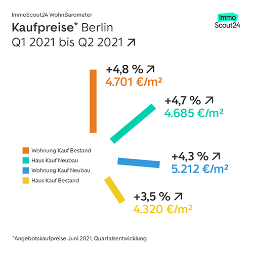
At ImmoScout24, our mission is to make complex decisions easy, and we realized that we needed a new concept to fulfill it. Instead of another index, we decided to build a market report that everyone can easily understand: the WohnBarometer. It’s based on our listings data and takes object properties into account. The key difference from the IMX is that the WohnBarometer shows rent and sale prices in Euro per square meter for specific residential real estate types over time. The figures therefore can be directly interpreted and allow our customers to answer questions such as “Do I pay too much rent?” or “Is the apartment I am about to buy reasonably priced?” or “Which city in my region is the most promising one for investing?” Currently, the WohnBarometer is reported for Germany as a whole, the seven biggest cities, and alternating local markets.

The following graph shows an example of the WohnBarometer, with sale prices for Berlin and the development per quarter.

This post discusses how ImmoScout24 used Amazon SageMaker to create the model for the WohnBarometer in order to make it relevant for our customers. It discusses the underlying data model, hyperparameter tuning, and technical setup. This post also shows how SageMaker supported one data scientist to complete the WohnBarometer within 2 months. It took a whole team 2 years to develop the first version of the IMX. Such an investment was not an option for the WohnBarometer.

About ImmoScout24

ImmoScout24 is the leading online platform for residential and commercial real estate in Germany. For over 20 years, ImmoScout24 has been revolutionizing the real estate market and supports over 20 million users each month on its online marketplace or in its app to find new homes or commercial spaces. That’s why 99% of our target customer group know ImmoScout24. With its digital solutions, the online marketplace coordinates and brings owners, realtors, tenants, and buyers together successfully. ImmoScout24 is working towards the goal of digitizing the process of real estate transactions and thereby making complex decisions easy. Since 2012, ImmoScout24 has also been active in the Austrian real estate market, reaching around 3 million users monthly.

From on-premises to AWS Data Pipeline to SageMaker

In this section, we discuss the previous setup and its challenges, and why we decided to use SageMaker for our new model.

The previous setup

When the first version of the IMX was published in 2010, the cloud was still a mystery to most businesses, including ImmoScout24. The field of machine learning (ML) was in its infancy and only a handful of experts knew how to code a model (for the sake of illustration, the first public release of Scikit-Learn was in February 2010). It’s no surprise that the development of the IMX took more than 2 years and cost a seven-figure sum.

In 2015, ImmoScout24 started its AWS migration, and rebuilt IMX on AWS infrastructure. With the data in our Amazon Simple Storage Service (Amazon S3) data lake, both the data preprocessing and the model training were now done on Amazon EMR clusters orchestrated by AWS Data Pipeline. While the former was a PySpark ETL application, the latter was several Python scripts using classical ML packages (such as Scikit-Learn).

Issues with this setup

Although this setup proved quite stable, troubleshooting the infrastructure or improving the model wasn’t easy. A key problem with the model was its complexity, because some components had begun a life on their own: in the end, the code of the outlier detection was almost twice as long the code of the core IMX model itself.

The core model, in fact, wasn’t one model, but hundreds: one model per residential real estate type and region, with the definition varying from a single neighborhood in a big city to several villages in rural areas. We had, for example, one model for apartments for sale in the middle of Berlin and one model for houses for sale in a suburb of Munich. Because setting up the training of all these models took a lot of time, we omitted the hyperparameter tuning, which likely led to the models underperforming.

Why we decided on SageMaker

Given these issues and our ambition of having a market report with practical benefits, we had to decide between rewriting large parts of the existing code or starting from scratch. As you can infer from this post, we opted for the latter. But why SageMaker?

Most of our time spent on the IMX went into troubleshooting the infrastructure, not improving the model. For the new market report, we wanted to flip this around, with the focus on the statistical performance of the model. We also wanted to have the flexibility to quickly replace individual components of the model, such as the optimization of the hyperparameters. What if a new superior boosting algorithm comes around (think about how XGBoost hit the stage in 2014)? Of course, we want to adopt it as one of the first!

In SageMaker, the major components of the classical ML workflow—preprocessing, training, hyperparameter tuning, and inference—are neatly separated on the API level and also on the AWS Management Console. Modifying them individually isn’t difficult.

The new model

In this section, we discuss the components of the new model, including its input data, algorithm, hyperparameter tuning, and technical setup.

Input data

The WohnBarometer is based on a sliding window of 5 years of ImmoScout24 listings of residential real estate located in Germany. After we remove outliers and fraudulent listings, we’re left with approximately 4 million listings that are split into train (60 %), validation (20 %), and test data (20 %). The relationship between listings and objects is not necessarily 1:1; over the course of 5 years, it’s likely that the same object is inserted multiple times (by multiple people).

We use 13 listing attributes, such as the location of the property (WGS84 coordinates), the real estate type (house or apartment, sale or rent), its age (years), its size (square meter) or it’s condition (for example, new or refurbished). Given that each listing typically comes with dozens of attributes, the question arises: which to include in the model? On the one hand, we used domain knowledge; for example, it’s well known that location is a key factor, and in almost all markets new property is more expensive than existing ones. On the other hand, we relied on our experiences with the IMX and similar models. There we learned that including dozens of attributes doesn’t significantly improve the model.

Depending on the real estate type of the listing, the target variable of our model is either the rent per square meter or the sale price per square meter (we explain later why this choice wasn’t ideal). Unlike the IMX, the WohnBarometer is therefore a number that can be directly interpreted and acted upon by our customers.

Model description

When using SageMaker, you can choose between different strategies of implementing your algorithm:

• Use one of SageMaker’s built-in algorithms. There are almost 20 and they cover all major ML problem types.
• Customize a pre-made Docker image based on a standard ML framework (such as Scikit-Learn or PyTorch).
• Build your own algorithm and deploy it as a Docker image.

For the WohnBarometer, we wanted a solution that is easy to maintain and allows us to focus on improving the model itself, not the underlying infrastructure. Therefore, we decided on the first option: use a fully-managed algorithm with proper documentation and fast support if needed. Next, we needed to pick the algorithm itself. Again, the decision wasn’t difficult: we went for the XGBoost algorithm because it’s one of the most renowned ML algorithms for regression type problems, and we have already successfully used it in several projects.

Hyperparameter tuning

Most ML algorithms come with a myriad of parameters to tweak. Boosting algorithms, for example, have many parameters specifying how exactly the trees are built: Do the trees have at maximum 20 or 30 leaves? Is each tree based on all rows and columns or only samples? How heavily to prune the trees? Finding the optimal values of those parameters (as measured by an evaluation metric of your choice), the so-called hyperparameter tuning, is critical to building a powerful ML model.

A key question in hyperparameter tuning is which parameters to tune and how to set the search ranges. You might ask, why not check all possible combinations? Although in theory this sounds like a good idea, it would result in an enormous hyperparameter space with way too many points to evaluate them all at a reasonable price. That is why ML practitioners typically select a small number of hyperparameters known to have a strong impact on the performance of the chosen algorithm.

After the hyperparameter space is defined, the next task is to find the best combination of values in it. The following techniques are commonly employed:

• Grid search – Divide the space in a discrete grid and then evaluate all points in the grid with cross-validation.
• Random search – Randomly draw combinations from the space. With this approach, you’ll most likely miss the best combination, but it serves as a good benchmark.
• Bayesian optimization – Build a probabilistic model of the objective function and use this model to generate new combinations. The model is updated after each combination, leading quickly to good results.

In recent years, thanks to cheap compute power, Bayesian optimization has become the gold standard in hyperparameter tuning, and is the default setting in SageMaker.

Technical setup

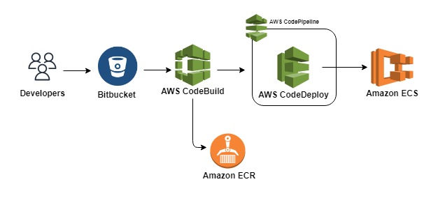
As with many other AWS services, you can create SageMaker jobs on the console, with the AWS Command Line Interface (AWS CLI), or via code. We chose the third option, the SageMaker Python SDK to be precise, because it allows for a highly automated setup: the WohnBarometer lives in a Python software project that is command-line executable. For example, all steps of the ML pipeline such as the preprocessing or the model training can be triggered via Bash commands. Those Bash commands, in turn, are orchestrated with a Jenkins pipeline powered by AWS Fargate.

Let’s look at the steps and the underlying infrastructure:

• Preprocessing – The preprocessing is done with the built-in Scikit-Learn library in SageMaker. Because it involves joining data frames with millions of rows, we need an ml.m5.24xlarge machine here, the largest you can get in the ml.m family. Alternatively, we could have used multiple smaller machines with a distributed framework like Dask, but we wanted to keep it as simple as possible.
• Training – We use the default SageMaker XGBoost algorithm. The training is done with two ml.m5.12xlarge machines. It’s worth mentioning that our train.py containing the code of the model training and the hyperparameter tuning has less than 100 rows.
• Hyperparameter tuning – Following the principle of less is more, we only tune 11 hyperparameters (for example, the number of boosting rounds and the learning rate), which gives us time to carefully choose their ranges and inspect how they interact with each other. With only a few hyperparameters, each training job runs relatively fast; in our case the jobs take between 10–20 minutes. With a maximal number of 30 training jobs and 2 concurrent jobs, the total training time is around 3 hours.
• Inference – SageMaker offers multiple options to serve your model. We use batch transform jobs because we only need the WohnBarometer numbers once a quarter. We didn’t use an endpoint because it would be idle most of the time. Each batch job (approximately 6.8 million rows) is served by a single ml.m5.4xlarge machine in less than 10 minutes.

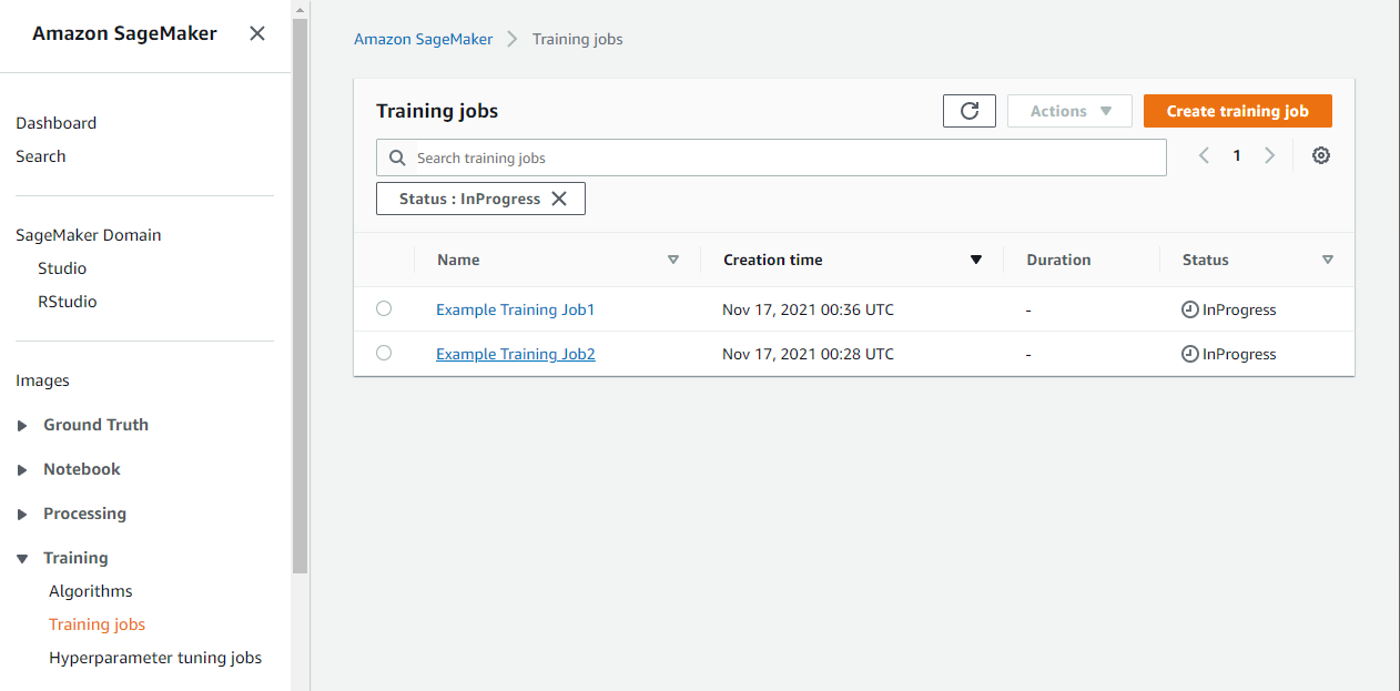
We can easily debug these steps on the SageMaker console. If, for example, a training job is taking longer than expected, we navigate to the Training page, locate the training job in question, and review Amazon CloudWatch metrics of the underlying machines.

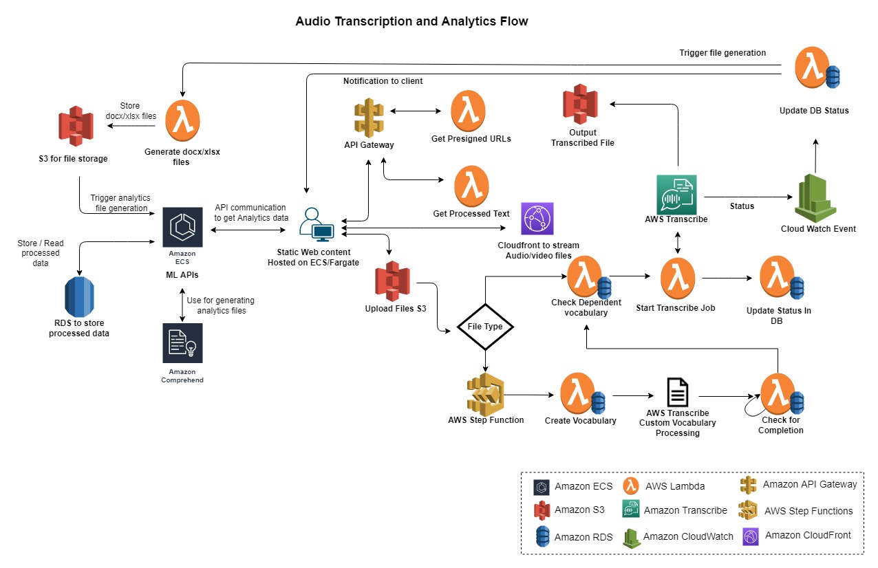
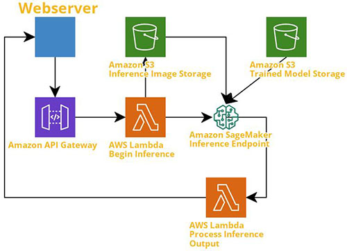
The following architecture diagram shows the infrastructure of the WohnBarometer:

Challenges and learnings

In the beginning everything went smoothly: within a few days we set up the software project and trained a miniature version of our model in SageMaker. We had high hopes for the first run on the full dataset and the hyperparameter tuning in place. Unfortunately, the results weren’t satisfying. We had the following key issues:

• The predictions of the model were too low, both for rent and sale objects. For Berlin, for example, the sale prices predicted for our reference objects were roughly 50% below the market prices.
• According to the model, there was no significant price difference between new and existing buildings. The truth is that new buildings are almost always significantly more expensive than existing buildings.
• The effect of the location on the price wasn’t captured correctly. We know, for example, that apartments for sale in Frankfurt am Main, are, on average, more expensive than in Berlin (although Berlin is catching up); our model, however, predicted it the other way round.

What was the problem and how did we solve it?

Sampling of the features

At first glance, it looks like the issues aren’t related, but indeed they are. By default, XGBoost builds each tree with a random sample of the features. Let’s say a model has 10 features F₁, F₂, … F₁₀, then the algorithm might use F₁, F₄, and F₇ for one tree, and F₃, F₄, and F₈ for another. While in general this behavior effectively prevents overfitting, it can be problematic if the number of features is small and some of them have a big effect on the target variable. In this case, many trees will miss the crucial features.

XGBoost’s sampling of our 13 features led to many trees including neither of the crucial features—real estate type, location, and new or existing buildings—and as a consequence caused these issues. Luckily, there is a parameter to control the sampling: colsample_bytree (in fact, there are two more parameters to control the sampling, but we didn’t touch them). When we checked our code, we saw that colsample_bytree was set to 0.5, a value we carried over from past projects. As soon as we set it to the default value of 1, the preceding issues were gone.

One model vs. multiple models

Unlike the IMX, the WohnBarometer model really is only one model. Although this minimizes the maintenance effort, it’s not ideal from a statistical point of view. Because our training data contains both sale and rent objects, the spread in the target variable is huge: it ranges from below 5 Euro for some rent apartments to well above 10,000 Euro for houses for sale in first-class locations. The big challenge for the model is to understand that an error of 5 Euro is fantastic for sale objects, but disastrous for rent objects.

In hindsight, knowing how easy it is to maintain multiple models in SageMaker, we would have built at least two models: one for rent and one for sale objects. This would make it easier to capture the peculiarities of both markets. For example, the price of unrented apartments for sale is typically 20–30% higher than for rented apartments for sale. Therefore, encoding this information as a dummy variable in the sale model makes a lot of sense; for the rent model on the other hand, you could leave it out.

Conclusion

Did the WohnBarometer meet the goal of being relevant to our customers? Taking media coverage as an indication, the answer is a clear yes: as of November 2021, more than 700 newspaper articles and TV or radio reports on the WohnBarometer have been published. The list includes national newspapers such as Frankfurter Allgemeine Zeitung, Tagesspiegel, and Handelsblatt, and local newspapers that often ask for WohnBarometer figures for their region. Because we calculate the figures for all regions of Germany anyway, we’re happy to take such requests. With the old IMX, this level of granularity wasn’t possible.

The WohnBarometer outperforms the IMX in regards to statical performance, in particular when it comes to the costs: the IMX was generated by an EMR cluster with 10 task nodes running almost half a day. In contrast, all WohnBarometer steps take less than 5 hours using medium-sized machines. This results in cost savings of almost 75%.

Thanks to SageMaker, we were able to bring a complex ML model in production with one data scientist in less than 2 months. This is remarkable. 10 years earlier, when ImmoScout24 built the IMX, reaching the same milestone took more than 2 years and involved a whole team.

How could we be so efficient? SageMaker allowed us to focus on the model instead of the infrastructure, and SageMaker promotes a microservice architecture that is easy to maintain. If we got stuck with something, we could call on AWS support. In the past, when one of our IMX data pipelines failed, we would sometimes spend days to debug it. Since we started publishing WohnBarometer figures in April 2021, the SageMaker infrastructure hasn’t failed a single time.

To learn more about the WohnBarometer, check out WohnBarometer and WohnBarometer: Angebotsmieten stiegen 2021 bundesweit wieder stärker an. To learn more about using the SageMaker Scikit-Learn library for preprocessing, see Preprocess input data before making predictions using Amazon SageMaker inference pipelines and Scikit-learn. Please send us feedback, either on the AWS forum for Amazon SageMaker, or through your AWS support contacts.

The content and opinions in this post are those of the third-party author and AWS is not responsible for the content or accuracy of this post.

About the Authors

Oliver Frost joined ImmoScout24 in 2017 as a business analyst. Two years later, he became a data scientist in a team whose job it is to turn ImmoScout24 data into veritable data products. Before building the WohnBarometer model, he ran smaller SageMaker projects. Oliver holds several AWS certificates, including the Machine Learning Specialty.

Lukas Müller is a Solutions Architect at AWS. He works with customers in the sports, media, and entertainment industries. He is always looking for ways to combine technical enablement with cultural and organizational enablement to help customers achieve business value with cloud technologies.

Read More

This post is authored by Satish Jha, Intelligent Automation Manager, Matt Docherty, Data Science Manager, Jayesh Muley, Associate Consultant and Tapan Vora, Rapid Prototyping, from ZS Associates.

At ZS Associates, we do a significant amount of qualitative market research. The work involves interviewing relevant subjects (such as healthcare professionals and sales representatives) and developing bespoke analytics on the interview data. We’ve taken advantage of the advances in AI, machine learning (ML), and cloud computing to reimagine qualitative market research and developed a scalable solution that is equipped to perform speech-to-text conversion and natural language processing (NLP) on the audio recordings of interviewed subjects. The solution is better, cheaper, and faster than the current ways of working (manual interpretation), giving a competitive advantage in this space.

This post discusses how ZS used Amazon Transcribe, Amazon Comprehend Medical, and custom NLP for text summarization and graph visualization to create a scalable, automated solution that helps us provide insights in a faster, better, and more efficient way.

Background assessment

The traditional method of performing qualitative market research requires human intervention and interpretation, which is highly subjective in nature. We used advanced AI and ML to develop a platform that is capable of the following:

• Performing speech-to-text conversion; specifically with high precision, converting interview audio recordings conducted for the purpose of qualitative market research
• Drawing analytical insights from the converted text using a state-of-the-art NLP model

To achieve this, we combined state-of-the-art AWS AI services and cloud computing capabilities with our propriety NLP and text summarization algorithms to drive impact at scale.

Solution overview

To build our solution, we adopted the methodology of starting small, highlighting value, and scaling fast. We identified a key user group and defined phase one of the solution to do automated speech-to-text and analytics. We defined a key user interface and developed the technology architecture for the solution. Because ZS is an AWS Partner and has already been using multiple AWS Cloud services for our enterprise products and solutions, AWS was the preferred choice for this project. We used Amazon Transcribe and Amazon Comprehend Medical for transcription and theme identification purposes. For hosting custom NLP analytics APIs, we used a serverless infrastructure using Amazon API Gateway, AWS Lambda, and Amazon Elastic Container Service (Amazon ECS) with AWS Fargate. These services are HIPAA-eligible and compliant with pharma regulatory requirements.

The process includes the following stages:

• File upload to Amazon S3 – The process starts when the user uploads one or more audio recording files for transcription to the site on which our tool is hosted. To upload the files to Amazon Simple Storage Service (Amazon S3), the user is provided with a temporary written token or pre-signed URL using API Gateway, which provides Amazon S3 access.
• Audio transcription – Depending on the type of file uploaded, different triggers are in place to initiate the appropriate workflow:
  • Audio files uploaded without a dictionary file – If the user didn’t provide a dictionary file, the tool processes the audio file using Amazon Transcribe.
  • Audio files uploaded with a dictionary file – If the user provided a dictionary file, certain AWS Step Functions steps are triggered, followed by processing the dictionary file using Amazon Transcribe. When the dictionary processing is complete, the tool transcribes the audio file using Amazon Transcribe.
• Transcript file generation – In either of the preceding two cases, when the transcription is in progress, the tool uses Amazon CloudWatch Events to update the transcription status. Lambda functions trigger the tool to update the status on the RDBMS and convey the status to the user through the tool’s UI using sockets. When the transcription is complete, the final output file is stored in Amazon S3.
• File type conversion – After the output file is generated, the tool uses triggers to create a .doc or .xlsx file, stored again in Amazon S3.
• Generating analytical insights – With Amazon Comprehend Medical and certain ZS in-house NLP tools, the tool generates analytics based on the transcribed data and updates dashboards on our site to access them in real time.
• Audio streaming with Amazon Transcribe – We use Amazon CloudFront audio streaming paired with our final output file, which is generated from Amazon Transcribe. The user can simultaneously listen to the recording and read the transcript.

The following diagram shows the high-level architecture and workflow.

The platform is designed to process a large number of files in real time. Therefore, the solution greatly augments the work of our current ZS qualitative research team by making the process more efficient and giving it an entirely new dimension!

Overall, our solution has the following features:

• The ability to upload single or multiple audio files
• Automated speech-to-text conversion, with the ability to add a custom dictionary
• The ability to listen to the uploaded audio and refine text
• Text summarization and analytics

Process map

The following diagram gives a high-level visualization of our developed solution, with the following stages:

• Upload audio – The process starts with the user uploading their audio recording (with or without a dictionary file) to the tool
• Speech to text – These uploaded audio files are transcribed by converting speech to text
• Listen and refine – The user can simultaneously listen to the recording and read the transcript and make changes wherever necessary
• Speech-to-text output – The consolidated file includes the converted transcript and its corresponding analytics

It took us approximately 5–6 months to develop this solution end to end with a four-member team. Today it is being used by over 300 people, and the tool has processed thousands of hours of audio.

AWS services used

The solution uses multiple AWs services:

• AWS Lambda and API Gateway – Hosted the serverless APIs and functions.
  • We developed multiple API Gateways to ensure loose coupling and easy integration with external APIs. Custom authorizers were implemented to enable token-based authentication and restrict unauthorized access to the web content.
  • We also built the Lambda APIs (using Python and NodeJS) that could easily interact with a website hosted on ECS containers and can also be easily linked with Amazon Relational Database Service (Amazon RDS) for PostgreSQL. The use of Lambda functions in our solution helped us avoid the load balancing, restoring, and stopping clusters efforts and reduce overall costs, because the clusters only ran when the functions were running. Additionally, we were able to easily scale our solution because of the serverless architecture.
• Amazon Transcribe – Provided us options to easily configure the batch processing of audio files up to 100 at a time and even scale a larger load using its built-in queuing mechanism. It also allowed us to load a custom dictionary to transcribe the audio data more accurately.
• Amazon Comprehend Medical – Generated analytical insights from the text data using its built-in NLP capabilities to sort through text for valuable information.
• AWS CloudFormation – We used AWS CloudFormation to deploy the Lambda functions and APIs across environments (various S3 buckets and multiple environments in the same bucket, such as production and development) using stage variables.
• AWS CodeBuild, AWS CodeDeploy, and AWS CodePipeline – We used AWS CodeBuild, AWS CodeDeploy, and AWS CodePipeline to perform continuous deployment of the front end and analytics backend to ECS clusters.

The following diagram illustrates the architecture of these services.

Conclusion

We used AWS services to develop a platform that helped our teams apply cutting-edge AI to their projects. It has helped our teams do the following:

• Automate the process of speech-to-text conversion and only focus on low-accuracy aspects.
• Drive automation of insights with NLP algorithms.
• Drive self-service. Because we do not need to launch any particular server, we can easily create Lambda functions, make changes to the code on the fly, and provide key ML services as plug and play so that users don’t need to be data scientists.

Today the solution is used by over 300 people, and we have processed thousands of hours of audio. We’re now integrating our solution with other applications to provide users with the flexibility to either upload audio files for transcription or directly upload transcribed files for drawing analytical insights.

We also derived multiple benefits from building our platform with AWS:

• Using an end-to-end cloud-based architecture proved beneficial in terms of managing environments for business applications
• With management tools such as CloudWatch, AWS CloudFormation, CodeBuild, CodeDeploy, and CodePipeline, it was easier to monitor, track, and deploy development changes
• We used AWS’s built-in security with virtual private clouds and identity management with customized policies
• We were able to reduce load on valuable microservices, with the additional benefit of quick hosting and deployment

About ZS

ZS Associates is a consulting and professional services firm focusing on consulting, software, and technology, headquartered in Evanston, Illinois, that provides services for clients in pharma, healthcare, and technology. The firm employs more than 10,000 employees in 30 offices in North America, South America, Europe, and Asia. ZS works with 49 of the 50 largest drug-makers and 17 of the 20 largest medical device makers and serves consumer products, financial services, industrial products, telecommunications, transportation, and logistics industries.

Disclaimer: AWS is not responsible for the content or accuracy of this post. The content and opinions in this post are solely those of the third-party author. It is each customers’ responsibility to determine whether they are subject to HIPAA, and if so, how best to comply with HIPAA and its implementing regulations. Before using AWS in connection with protected health information, customers must enter an AWS Business Associate Addendum (BAA) and follow its configuration requirements.

About the Authors

Satish Jha is a Manager with ZS Associates. He is a leader in the firm’s Intelligent Automation Practice, where he works side by side with several pharma clients to transform operations and drive impact.

Matt Docherty is a Data Science Manager with ZS Associates in the Philadelphia office. He is focused on applying data science in the pharmaceutical industry.

Jayesh Muley is an Associate Consultant for Process Excellence & Transformation with ZS Associates. He has 4 years of experience advising pharma clients in the forecasting, process excellence, and digital transformation spaces. He played a critical role in establishing ZS’s automation center of excellence. He is always keen on learning new technologies and is always evolving in his role.

Tapan Vora is a Manager for Rapid Prototyping with ZS Associates. Tapan has over 14 years of technology and engineering management experience. He plays multiple roles in the team, such as business analyst, people manager, solution designer, data analyst, and product leader.

Read More