As an applied science manager at Amazon, Muthu Chandrasekaran works on new tools to automate and build a risk technology.Read More
Amazon VP Babak Parviz appointed to AAAS Board of Directors
Parviz will serve a three-year term as one of four appointed directors.Read More
Bundesliga Match Fact Set Piece Threat: Evaluating team performance in set pieces on AWS
The importance of set pieces in football (or soccer in the US) has been on the rise in recent years: now more than one quarter of all goals are scored via set pieces. Free kicks and corners generally create the most promising situations, and some professional teams have even hired specific coaches for those parts of the game.
In this post, we share how the Bundesliga Match Fact Set Piece Threat helps evaluate performance in set pieces. As teams look to capitalize more and more on these dead ball situations, Set Piece Threat will help the viewer understand how well teams are leveraging these situations. In addition, it will explain the reader how AWS services can be used to compute statistics in real-time.
Bundesliga’s Union Berlin is a great example for the relevance of set pieces. The team managed to rise from Bundesliga 2 to qualification for a European competition in just 2 years. They finished third in Bundesliga 2 during the 18/19 season, earning themselves a slot in the relegation playoffs to the Bundesliga. In that season, they scored 28 goals from open play, ranking just ninth in the league. However, they ranked second for goals scored through set pieces (16 goals).
Tellingly, in the first relegation playoff match against VfB Stuttgart, Union secured a 2:2 draw, scoring a header after a corner. And in the return match, Stuttgart was disallowed a free kick goal due to a passive offside, allowing Union to enter the Bundesliga with a 0:0 draw.
The relevance of set pieces for Union’s success doesn’t end there. Union finished their first two Bundesliga seasons with strong eleventh and seventh, ranking third and first in number of set piece goals (scoring 15 goals from set pieces in both seasons). For comparison, FC Bayern München—the league champion—only managed to score 10 goals from set pieces in both seasons. The success that Union Berlin has had with their set pieces allowed them to secure the seventh place in the 20/21 Bundesliga season, which meant qualification for the UEFA Europa Conference League, going from Bundesliga 2 to Europe just 2 years after having earned promotion. Unsurprisingly, in the deciding match, they scored one of their two goals after a corner. At the time of this writing, Union Berlin ranks fourth in the Bundesliga (matchday 20) and first in corner performance, a statistic we explain later.
Union Berlin’s path to Europe clearly demonstrates the influential role of offensive and defensive performance during set pieces. Until now however, it was difficult for fans and broadcasters to properly quantify this performance, unless they wanted to dissect massive tables on analytics websites. Bundesliga and AWS have worked together to illustrate the threat that a team produces and the threat that is produced by set pieces against the team, and came up with the new Bundesliga Match Fact: Set Piece Threat.
How does Set Piece Threat work?
To determine the threat a team poses with their set pieces, we take into account different facets of their set piece performance. It’s important to note that we only consider corners and free kicks as set pieces, and compute the threat for each category independently.
Facet 1: Outcome of a set piece: Goals, shots, or nothing
First, we consider the outcome of a set piece. That is, we observe if it results in a goal. However, the outcome is generally influenced by fine margins, such as a great save by the goal keeper or if a shot brushes the post instead of going in, so we also categorize the quality of a shot that results from the set piece. Shots are categorized into several categories.
| Category | Explanation |
| Goal | A successful shot that lead to a goal |
| Outstanding | Shots that almost led to a goal, such as a shot at the post |
| Decent | Other noteworthy goals scenes |
| Average | The rest of the chances that would be included in a chances ratio with relevant threat of a goal |
| None | No real goal threat, should not be considered a real chance, such as a header that barely touched the ball or a blocked shot |
| No shot | No shots taken at all |
The above video shows examples of shot outcome categories in the following order: outstanding, decent, average, none.
Facet 2: Potential of a shot
Second, our algorithm considers the potential of a shot. This incorporates how likely it should have resulted in a goal, taking the actual performance of the shot-taker out of the equation. In other words, we quantify the goal potential of the situation in which the shot was taken. This is captured by the expected goal (xGoals) value of the shot. We remove not only the occurrence of luck or lack thereof, but also the quality of the strike or header.

Facet 3: Quantity of set pieces
Next, we consider the aspect of pure quantity of set pieces that a team gets. Our definition of Set Piece Threat measures the threat on a per-set-piece-basis. Instead of summing up all outcomes and xGoal values of a team over the course of a season, the values are aggregated such that they represent the average threat per set piece. That way, the corner threat, for example, represents the team’s danger for each corner and doesn’t consider a team more dangerous simply because they have more corners than other teams (and therefore potentially more shots or goals).
Facet 4: Development over time
The last aspect to consider is the development of a team’s threat over time. Consider for example a team that scored three goals from corners in the first three matchdays but fails to deliver any considerable threat over the next 15 matchdays. This team should not be considered to pose a significant threat from corners on matchday 19, despite it already having scored three times, which may still be a good return. We account for this (positive or negative) development of a team’s set piece quality by assigning a discount to each set piece, depending on how long ago it occurred. In other words, a free kick that was taken 10 matchdays ago has less influence on the computed threat than one that was taken during the last or even current game.
Score: Per set piece aggregation
All four facets we’ve described are aggregated into two values for each team, one for corners and one for free kicks, which describe the danger that a corresponding set piece by that team would currently pose. The value is defined as the weighted average of the scores of each set piece, where the score of a set piece is defined as (0.7 * shot-outcome + 0.3 * xG-value) if the set piece resulted in a shot and 0 otherwise. The shot-outcome is 1 if the team scored and lower for other outcomes, such as a shot that went wide, depending on its quality. The weight for each set piece is determined by how long ago it was taken, as described earlier. Overall, the values are defined between 0–1, where 1 is the perfect score.

Set piece threat
Next, the values for each team are compared to the league average. The exact formula is score(team)/avg_score(league) - 1. This value is what we call the Set Piece Threat value. A team has a threat value of 0 if it’s exactly as good as the league average. A value of -1 (or -100%) describes a team that poses no threat at all, and a value of +1 (+100%) describes a team that is twice as dangerous as the league average. With those values, we compute a ranking that orders the teams from 1–18 according to their offensive threat of corners and free kicks, respectively.
 |
 |
We use the same data and similar calculations to also compute a defensive threat that measures the defensive performance of a team with regard to how they defend set pieces. Now, instead of computing a score per own set piece, the algorithm computes a score per opponent set piece. Just like for the offensive threat, the score is compared to the league average, but the value is reversed: -score(team)/avg_score(league) + 1. This way, a threat of +1 (+100%) is achieved if team allows opponents no shots at all, whereas a team with defensive threat of -1 (-100%) is twice as susceptible to opponents’ set pieces as the league average. Again, a team with a threat of 0 is as good as the league average.


Set Piece Threat findings
An important aspect of Set Piece Threat is that we focus on an estimation of threat instead of goals scored and conceded via set pieces. If we take SC Freiburg and Union Berlin at matchday 21 as an example, over the course of this season Freiburg has scored seven goals via corners in comparison to four from Union Berlin. Our threat ranking still ranks both of the teams fairly equal. In fact, we predict a corner by Freiburg (Rank 3) to even be 7% less threatening than a corner by Union Berlin (Rank 1). The main reason for this is that Union Berlin created a similar number of great chances out of their corners, but failed to convert these chances into goals. Freiburg on the other hand was vastly more efficient with their chances. Such a discrepancy between chance quality and actual goals can happen in a high-variance sport like football.
The following graph shows Union Berlin’s set piece offensive corner ranking (blue) and score (red) from matchdays 6–21. At matchday 12, Union scored a goal from a corner and additionally had a great chance from a second corner that didn’t result in a goal but was perceived as a high threat by our algorithm. In addition, Union had a shot on target in five of seven corner kicks on matchday 12. Union immediately jumped in the ranking from twelfth to fifth place as a result of this, and the score value for Union increased as well as the league average. As Union saw more and more high threat chances in the later matchdays from corners, they step by step claimed first place of the corner threat ranking. The score is always relative to the current league average, meaning that Union’s threat at matchday 21 is 50% higher from corners than the average threat coming from all teams in the league.

Implementation and architecture
Bundesliga Match Facts are independently running AWS Fargate containers inside Amazon Elastic Container Service (Amazon ECS). Previous Bundesliga Match Facts consume raw event and positional data to calculate advanced statistics. This changes with the release of Set Piece Threat, which analyzes data produced by an existing Bundesliga Match Fact (xGoals) to calculate its rankings. Therefore, we created an architecture to exchange messages between different Bundesliga Match Facts during live matches in real time.
To guarantee the latest data is reflected in the set piece threat calculations, we use Amazon Managed Streaming for Apache Kafka (Amazon MSK). This message broker service allows different Bundesliga Match Facts to send and receive the newest events and updates in real time. By consuming a match and Bundesliga Match Fact-specific topic from Kafka, we can receive the most up-to-date data from all systems involved while retaining the ability to replay and reprocess messages sent earlier.
The following diagram illustrates the solution architecture:

We introduced Amazon MSK to this project to generally replace all internal message passing for the Bundesliga Match Facts platform. It handles the injection of positional and event data, which can aggregate to over 3.6 million data points per match. With Amazon MSK, we can use the underlying persistent storage of messages, which allows us to replay games from any point in time. However, for Set Piece Threat, the focus lies on the specific use case of passing events produced by Bundesliga Match Facts to other Bundesliga Match Facts that are running in parallel.
To facilitate this, we distinguish between two types of Kafka topics: global and match-specific. First, each Bundesliga Match Fact has an own specific global topic, which handles all messages created by the Bundesliga Match Fact. Additionally, there is an additional match-specific topic for each Bundesliga Match Fact for each match that is handling all messages created by a Bundesliga Match Fact for a specific match. When multiple live matches run in parallel, each message is first produced and sent to this Bundesliga Match Fact-specific global topic.
A dispatcher AWS Lambda function is subscribed to every Bundesliga Match Fact-specific global topic and has two tasks:
- Write the incoming data to a database provisioned through Amazon Relational Database Service (Amazon RDS).
- Redistribute the messages that can be consumed by other Bundesliga Match Facts to a Bundesliga Match Fact-specific topic.
The left side of the architecture diagram shows the different Bundesliga Match Facts running independently from each other for every match and producing messages to the global topic. The new Set Piece Threat Bundesliga Match Fact now can consume the latest xGoal values for each shot for a specific match (right side of the diagram) to immediately compute the threat produced by the set piece that resulted in one or more shots.
Summary
We’re excited about the launch of Set Piece Threat and the patterns commentators and fans will uncover using this brand-new insight. As teams look to capitalize more and more on these dead ball situations, Set Piece Threat will help the viewer understand which team is doing this successfully and which team still has some ground to cover, which adds additional suspense before each of these set piece situations. The new Bundesliga Match Fact is available to Bundesliga’s broadcasters to uncover new perspectives and stories of a match, and team rankings can be viewed at any time in the Bundesliga app.
We’re excited to learn what patterns you will uncover. Share your insights with us: @AWScloud on Twitter, with the hashtag #BundesligaMatchFacts.
About the Authors
Simon Rolfes played 288 Bundesliga games as a central midfielder, scored 41 goals and won 26 caps for Germany. Currently Rolfes serves as Sporting Director at Bayer 04 Leverkusen where he oversees and develops the pro player roster, the scouting department and the club’s youth development. Simon also writes weekly columns on Bundesliga.com about the latest Bundesliga Match Facts powered by AWS
Luuk Figdor is a Senior Sports Technology Specialist in the AWS Professional Services team. He works with players, clubs, leagues, and media companies such as Bundesliga and Formula 1 to help them tell stories with data using machine learning. In his spare time, he likes to learn all about the mind and the intersection between psychology, economics, and AI.
Jan Bauer is a Cloud Application Architect at AWS Professional Services. His interests are serverless computing, machine learning, and everything that involves cloud computing. He works with clients across industries to help them be successful on their cloud journey.
Pascal Kühner is a Cloud Application Developer in the AWS Professional Services Team. He works with customers across industries to help them achieve their business outcomes via application development, DevOps, and infrastructure. He loves ball sports and in his spare time likes to play basketball and football.
Uwe Dick is a Data Scientist at Sportec Solutions AG. He works to enable Bundesliga clubs and media to optimize their performance using advanced stats and data—before, after, and during matches. In his spare time, he settles for less and just tries to last the full 90 minutes for his recreational football team.
Javier Poveda-Panter is a Data Scientist for EMEA sports customers within the AWS Professional Services team. He enables customers in the area of spectator sports to innovate and capitalize on their data, delivering high quality user and fan experiences through machine learning and data science. He follows his passion for a broad range of sports, music and AI in his spare time.
Bundesliga Match Fact Skill: Quantifying football player qualities using machine learning on AWS
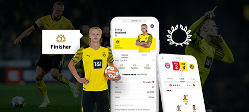
In football, as in many sports, discussions about individual players have always been part of the fun. “Who is the best scorer?” or “Who is the king of defenders?” are questions perennially debated by fans, and social media amplifies this debate. Just consider that Erling Haaland, Robert Lewandowski, and Thomas Müller alone have a combined 50 million followers on Instagram. Many fans are aware of the incredible statistics star players like Lewandowski and Haaland create, but stories like this are just the tip of the iceberg.
Consider that almost 600 players are under contract in the Bundesliga, and each team has their own champions—players that get introduced to bring a specific skill to bear in a match. Look for example at Michael Gregoritsch of FC Augsburg. As of this writing (matchday 21), he has scored five goals in the 21/22 season, not something that would make anybody mention him in a conversation about the great goal scorers. But let’s look closer: if you accumulate the expected goal (xGoals) values of all scoring chances Gregoritsch had this season, the figure you get is 1.7. This means he over-performed on his shots on goal by +194%, scoring 3.2 more goals than expected. In comparison, Lewandowski over-performed by only 1.6 goals (+7%). What a feat! Clearly Gregoritsch brings a special skill to Augsburg.
So how do we shed light on all the hidden stories about individual Bundesliga players, their skills, and impact on match outcomes? Enter the new Bundesliga Match Fact powered by AWS called Skill. Skill has been developed through in-depth analysis by the DFL and AWS to identify players with skills in four specific categories: initiator, finisher, ball winner, and sprinter. This post provides a deep dive into these four skills and discusses how they are implemented on AWS infrastructure.
Another interesting point is that until now, Bundesliga Match Facts have been developed independent from one another. Skill is the first Bundesliga Match Fact that combines the output of multiple Bundesliga Match Facts in real time using a streaming architecture built on Amazon Managed Streaming Kafka (Amazon MSK).
Initiator
An initiator is a player who performs a high number of valuable first and second assists. To identify and quantify the value of those assists, we introduced the new metric xAssist. It’s calculated by tracking the last and second-last pass before a shot at goal, and assigning the respective xGoals value to those actions. A good initiator creates opportunities under challenging circumstances by successfully completing passes with a rate of high difficulty. To evaluate how hard it is to complete a given pass, we use our existing xPass model. In this metric, we purposely exclude crosses and free kicks to focus on players who generate scoring chances with their precise assists from open play.
The skill score is calculated with the following formula:

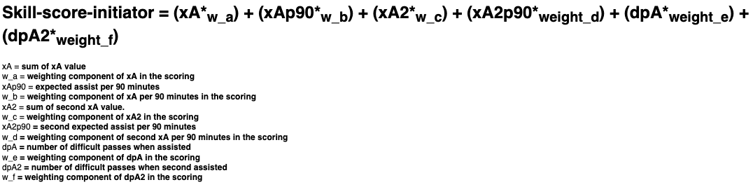
Let’s look at the current Rank 1 initiator, Thomas Müller, as an example. He has collected an xAssist value of 9.23 as of this writing (matchday 21), meaning that his passes for the next players who shot at the goal have generated a total xGoal value of 9.23. The xAssist per 90 minutes ratio is 0.46. This can be calculated from his total playing time of the current season, which is remarkable—over 1,804 minutes of playing time. As a second assist, he generated a total value of 3.80, which translates in 0.19 second assists per 90 minutes. In total, 38 of his 58 first assists were difficult passes. And as a second assist, 11 of his 28 passes were also difficult passes. With these statistics, Thomas Müller has catapulted himself into first place in the initiator ranking. For comparison, the following table presents the values of the current top three.
| .. | xAssist | xAssistper90 | xSecondAssist | xSecondAssistper90 | DifficultPassesAssisted | DifficultPassesAssisted2 | Final Score |
| Thomas Müller – Rank 1 | 9.23 | 0.46 | 3.80 | 0.18 | 38 | 11 | 0.948 |
| Serge Gnabry – Rank 2 | 3.94 | 0.25 | 2.54 | 0.16 | 15 | 11 | 0.516 |
| Florian Wirtz – Rank 3 | 6.41 | 0.37 | 2.45 | 0.14 | 21 | 1 | 0.510 |
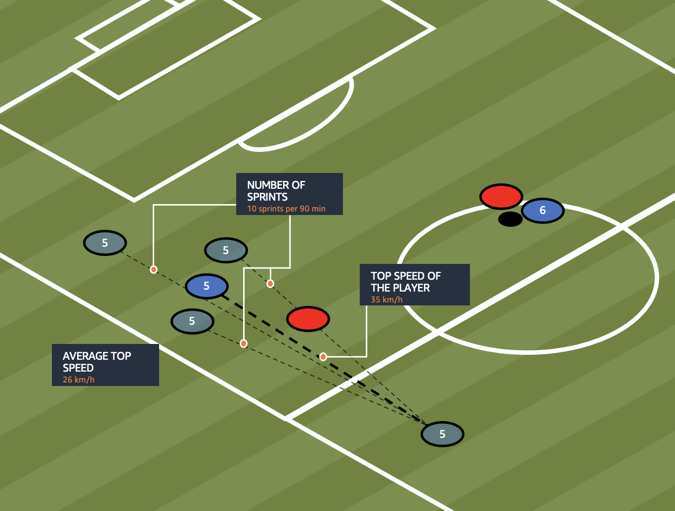
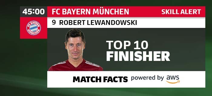
Finisher
A finisher is a player who is exceptionally good at scoring goals. He has a high shot efficiency and accomplishes many goals respective to his playing time. The skill is based on actual goals scored and its difference to expected goals (xGoals). This allows us to evaluate whether chances are being well exploited. Let’s assume that two strikers have the same number of goals. Are they equally strong? Or does one of them score from easy circumstances while the other one finishes in challenging situations? With shot efficiency, this can be answered: if the goals scored exceed the number of xGoals, a player is over-performing and is a more efficient shooter than average. Through the magnitude of this difference, we can quantify the extent to which a shooter’s efficiency beats the average.
The skill score is calculated with the following formula:
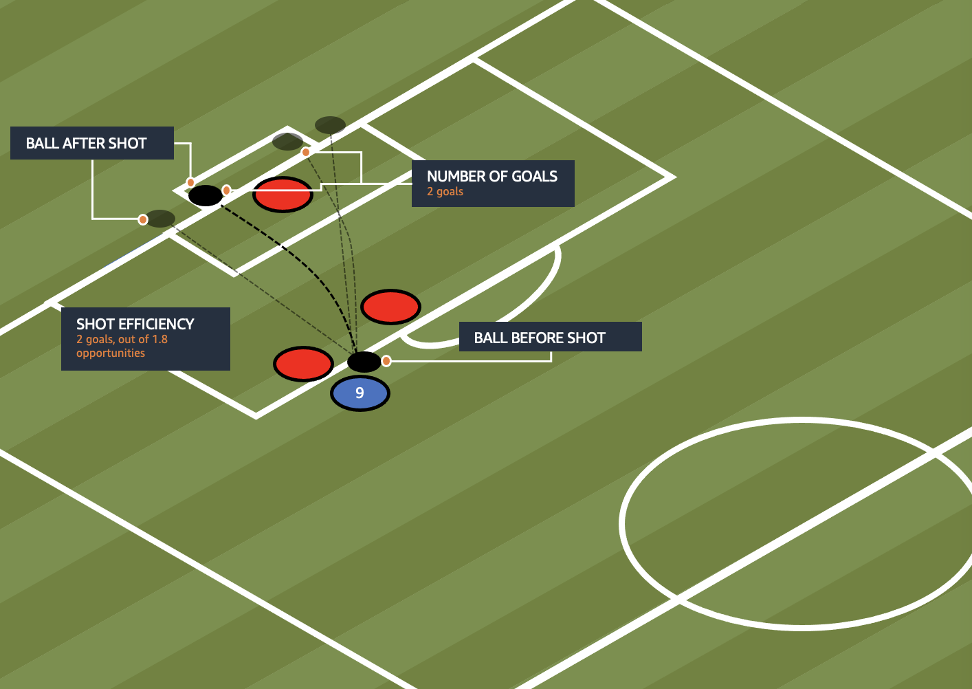
For the finisher, we focus more on goals. The following table gives a closer look at the current top three.
| .. | Goals | GoalsPer90 | ShotEfficiency | Final Score |
| Robert Lewandowski – Rank 1 | 24 | 1.14 | 1.55 | 0.813 |
| Erling Haaland – Rank 2 | 16 | 1.18 | 5.32 | 0.811 |
| Patrik Schick – Rank 3 | 18 | 1.10 | 4.27 | 0.802 |
Robert Lewandowski has scored 24 goals this season, which puts him in first place. Although Haaland has a higher shot efficiency, it’s still not enough for Haaland to be ranked first, because we give higher weighting to goals scored. This indicates that Lewandowski profits highly from both the quality and quantity of received assists, even though he scores exceptionally well. Patrick Schick has scored two more goals than Haaland, but has a lower goal per 90 minutes rate and a lower shot efficiency.
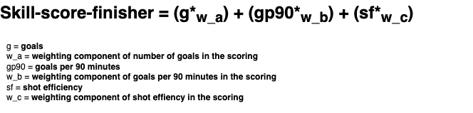
Sprinter
The sprinter has the physical ability to reach high top speeds, and do so more often than others. For this purpose, we evaluate average top speeds across all games of a player’s current season and include the frequency of sprints per 90 minutes, among other metrics. A sprint is counted if a player runs at a minimum pace of 4.0 m/s for more than two seconds, and reaches a peak velocity of at least 6.3 m/s during this time. The duration of the sprint is characterized by the time between the first and last time the 6.3 m/s threshold is reached, and needs to be at least 1 second long to be acknowledged. A new sprint can only be considered to have occurred after the pace had fallen below the 4.0 m/s threshold again.
The skill score is calculated with the following formula:
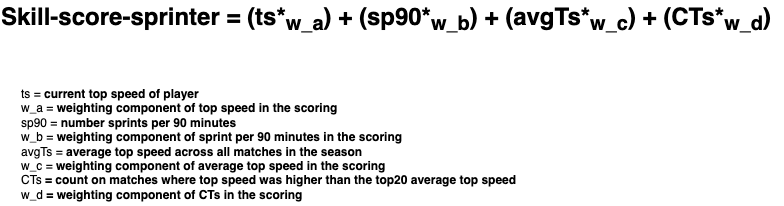
The formula allows us to evaluate the many ways we can look at sprints by players, and go further than just looking at the top speeds these players produce. For example, Jeremiah St. Juste has the current season record of 36.65 km/h. However, if we look at the frequency of his sprints, we find he only sprints nine times on average per match! Alphonso Davies on the other hand might not be as fast as St. Juste (top speed 36.08 km/h), but performs a staggering 31 sprints per match! He sprints much more frequently at with a much higher average speed, opening up space for his team on the pitch.
Ball winner
A player with this ability causes ball losses to the opposing team, both in total and respective to his playing time. He wins a high number of ground and aerial duels, and he steals or intercepts the ball often, creating a safe ball control himself, and a possibility for his team to counterattack.
The skill score is calculated with the following formula:
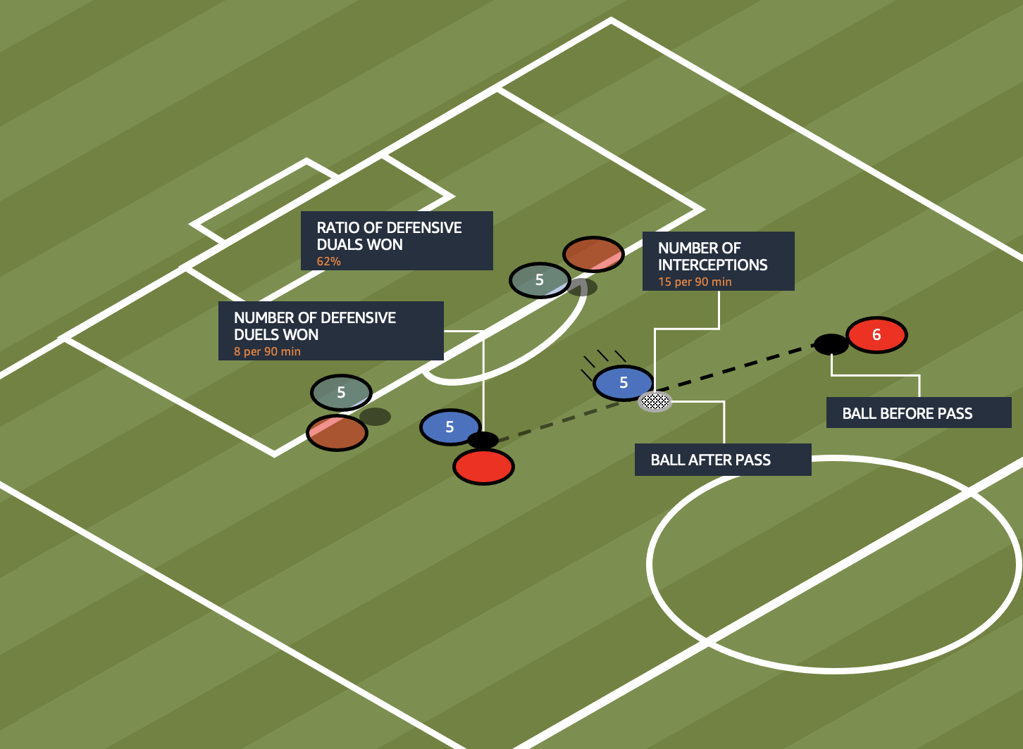
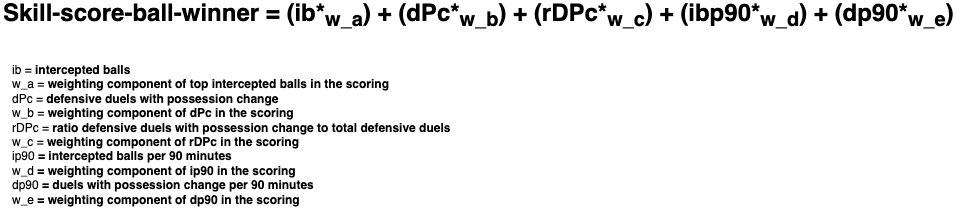
As of this writing, the first place ball winner is Danilo Soares. He has a total of 235 defensive duels. Of the 235 defensive duels, he has won 75, defeating opponents in a face-off. He has intercepted 51 balls this season in his playing position as a defensive back, giving him a win rate of about 32%. On average, he intercepted 2.4 balls per 90 minutes.
Skill example
The Skill Bundesliga Match Fact enables us to unveil abilities and strengths of Bundesliga players. The Skill rankings put players in the spotlight that might have gone unnoticed before in rankings of conventional statistics like goals. For example, take a player like Michael Gregoritsch. Gregoritsch is a striker for FC Augsburg who placed sixth in the finisher ranking as of matchday 21. He has scored five goals so far, which wouldn’t put him at the top of any goal scoring ranking. However, he managed to do this in only 663 minutes played! One of these goals was the late equalizer in the 97th minute that helped Augsburg to avoid the away loss in Berlin.
Through the Skill Bundesliga Match Fact, we can also recognize various qualities of each player. One example of this is the Dortmund star Erling Haaland, who has also earned the badge of sprinter and finisher, and is currently placed sixth amongst Bundesliga sprinters.
 |
 |
 |
 |
All of these metrics are based on player movement data, goal-related data, ball action-related data, and pass-related data. We process this information in data pipelines and extract the necessary relevant statistics per skill, allowing us to calculate the development of all metrics in real time. Many of the aforementioned statistics are normalized by time on the pitch, allowing for the consideration of players who have little playing time but perform amazingly well when they play. The combinations and weights of the metrics are combined into a single score. The result is a ranking for all players on the four player skills. Players ranking in the top 10 receive a skill badge to help fans quickly identify the exceptional qualities they bring to their squads.

Implementation and architecture
Bundesliga Match Facts that have been developed up to this point are independent from one another and rely only on the ingestion of positional and event data, as well as their own calculations. However, this changes for the new Bundesliga Match Fact Skill, which calculates skill rankings based on data produced by existing Match Facts, as for example xGoals or xPass. The outcome of one event, possibly an incredible goal with low chances of going in, can have a significant impact on the finisher skill ranking. Therefore, we built an architecture that always provides the most up-to-date skill rankings whenever there is an update to the underlying data. To achieve real-time updates to the skills, we use Amazon MSK, a managed AWS service for Apache Kafka, as a data streaming and messaging solution. This way, different Bundesliga Match Facts can communicate the latest events and updates in real time.
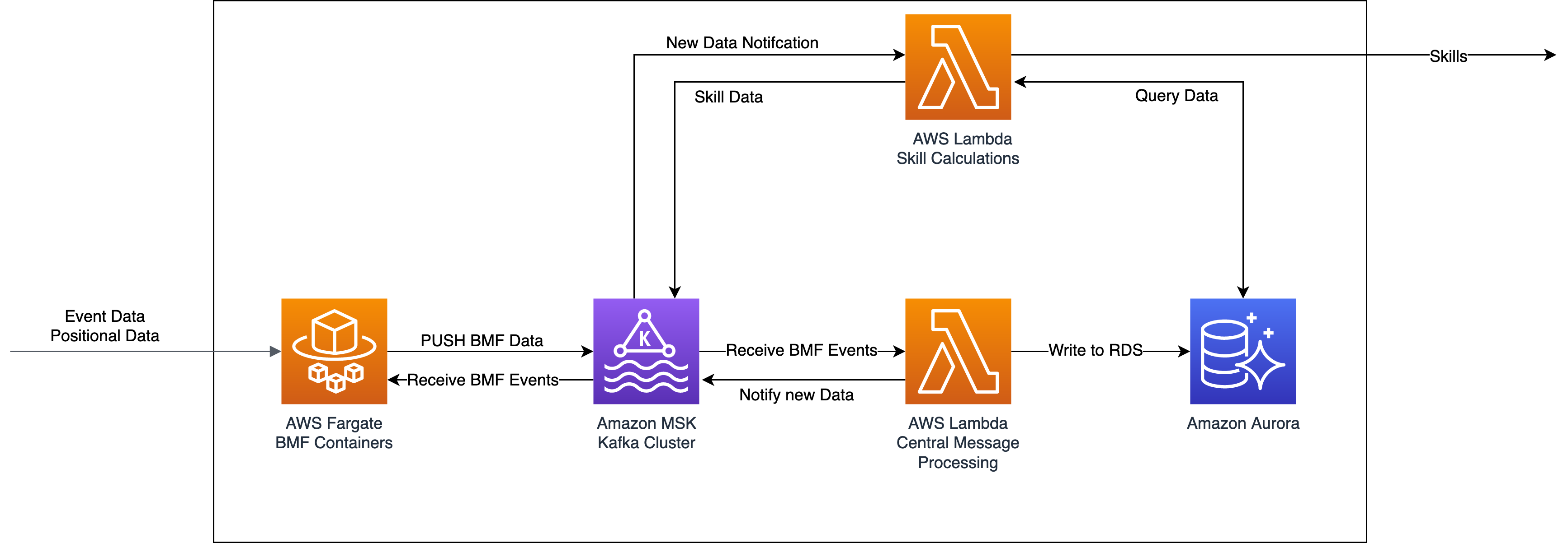
The underlying architecture for Skill consists of four main parts:
- An Amazon Aurora Serverless cluster stores all outputs of existing match facts. This includes, for example, data for each pass (such as xPass, player, intended receiver) or shot (xGoal, player, goal) that has happened since the introduction of Bundesliga Match Facts.
- A central AWS Lambda function writes the Bundesliga Match Fact outputs into the Aurora database and notifies other components that there has been an update.
- A Lambda function for each individual skill computes the skill ranking. These functions run whenever new data is available for the calculation of the specific skill.
- An Amazon MSK Kafka cluster serves as a central point of communication between all these components.
The following diagram illustrates this workflow. Each Bundesliga Match Fact immediately sends an event message to Kafka whenever there is an update to an event (such as an updated xGoals value for a shot event). The central dispatcher Lambda function is automatically triggered whenever a Bundesliga Match Fact sends such a message and writes this data to the database. Then it sends another message via Kafka containing the new data back to Kafka, which serves as a trigger for the individual skill calculation functions. These functions use data from this trigger event, as well as the underlying Aurora cluster, to calculate and publish the newest skill rankings. For a more in-depth look into the use of Amazon MSK within this project, refer to the Set Piece Threat blogpost.
Summary
In this post, we demonstrated how the new Bundesliga Match Fact Skill makes it possible to objectively compare Bundesliga players on four core player dimensions, building on and combining former independent Bundesliga Match Facts in real time. This allows commentators and fans alike to uncover previously unnoticed player abilities and shed light on the roles that various Bundesliga players fulfill.
The new Bundesliga Match Fact is the result of an in-depth analysis by the Bundesliga’s football experts and AWS data scientists to distill and categorize football player qualities based on objective performance data. Player skill badges are shown in the lineup and on player detail pages in the Bundesliga app. In the broadcast, player skills are provided to commentators through the data story finder and visually shown to fans at player substitution and when a player moves up into the respective top 10 ranking.
We hope that you enjoy this brand-new Bundesliga Match Fact and that it provides you with new insights into the game. To learn more about the partnership between AWS and Bundesliga, visit Bundesliga on AWS!
About the Authors
Simon Rolfes played 288 Bundesliga games as a central midfielder, scored 41 goals and won 26 caps for Germany. Currently Rolfes serves as Sporting Director at Bayer 04 Leverkusen where he oversees and develops the pro player roster, the scouting department and the club’s youth development. Simon also writes weekly columns on Bundesliga.com about the latest Bundesliga Match Facts powered by AWS
Luuk Figdor is a Senior Sports Technology Specialist in the AWS Professional Services team. He works with players, clubs, leagues, and media companies such as the Bundesliga and Formula 1 to help them tell stories with data using machine learning. In his spare time, he likes to learn all about the mind and the intersection between psychology, economics, and AI.
Pascal Kühner is a Cloud Application Developer in the AWS Professional Services Team. He works with customers across industries to help them achieve their business outcomes via application development, DevOps, and infrastructure. He is very passionate about sports and enjoys playing basketball and football in his spare time.
Tareq Haschemi is a consultant within AWS Professional Services. His skills and areas of expertise include application development, data science, machine learning, and big data. Based in Hamburg, he supports customers in developing data-driven applications within the cloud. Prior to joining AWS, he was also a consultant in various industries such as aviation and telecommunications. He is passionate about enabling customers on their data/AI journey to the cloud.
Jakub Michalczyk is a Data Scientist at Sportec Solutions AG. Several years ago, he chose math studies over playing football, as he came to the conclusion, he was not good enough at the latter. Now he combines both these passions in his professional career by applying machine learning methods to gain a better insight into this beautiful game. In his spare time, he still enjoys playing seven-a-side football, watching crime movies, and listening to film music.
Javier Poveda-Panter is a Data Scientist for EMEA sports customers within the AWS Professional Services team. He enables customers in the area of spectator sports to innovate and capitalize on their data, delivering high-quality user and fan experiences through machine learning and data science. He follows his passion for a broad range of sports, music, and AI in his spare time.
Announcing the AWS DeepRacer League 2022
Unleash the power of machine learning (ML) through hands-on learning and compete for prizes and glory. The AWS DeepRacer League is the world’s first global autonomous racing competition driven by reinforcement learning; bringing together students, professionals, and enthusiasts from almost every continent.
I’m Tomasz Ptak, a senior software engineer at Duco, an AWS Machine Learning Hero, an AWS DeepRacer competitor (named Breadcentric), a hobbyist baker, and a leader of the AWS Machine Learning Community on Slack, where we learn, race, and help each other start and grow our adventures in the cloud. It’s my pleasure to unveil the exciting details of the upcoming 2022 AWS DeepRacer League season.
What is AWS DeepRacer?
AWS DeepRacer is a 1/18th scale autonomous race car—but also much more. It’s a complete program that has helped over 175,000 individuals from over 700 businesses, educational institutions, and organizations begin their educational journey into machine learning through fun and rivalry.

AWS DeepRacer League 2022
Over 100,000 developers took part in the 2021 season of the AWS DeepRacer League. They got hands-on with reinforcement learning by participating in a workshop or training a model to achieve the fastest lap on the eight monthly global leaderboards. The monthly winners from these races joined us for the fully virtual 2021 Championship during the month of November, with the head-to head live finale taking place on November 23, 2021.
Due to restrictions on global travel in 2021, the entire AWS DeepRacer League was hosted within the Virtual Circuit. Although it made for entertaining livestream events that brought racers together each month from around the globe, it’s my opinion that nothing compares to the excitement of bringing the community together to race in person in the same room. That’s why I’m so thrilled that in 2022, the AWS DeepRacer League Summit Circuit will be back with 17 stops across five continents. We will learn the exact number of races after the AWS Summits dates are announced.
New in 2022, the AWS Summit Circuit structure is fully revamped, adding new regional playoffs coming this fall on the AWS Twitch channel. The top two competitors of each AWS Summit event will advance to the regional playoff round, where they will compete with other developers from their region for a chance to win a trip to Las Vegas to compete in the Championship Cup at AWS re:Invent 2022. In total, 15 participants from the AWS Summit Circuit regional playoffs will advance to the AWS DeepRacer League Championships. More on that later in this post.
That’s not all—anyone can participate in the AWS DeepRacer League Virtual Circuit races, the first of which is starting today, March 1, 2022. The Virtual Circuit consists of 8 months of racing in two divisions: Open and Pro. All racers start in the Open Division (except for the top three champions from 2021), competing in time trial races. At the end of each month, the top 10% of racers in the Open Division will advance to the pros and win a Pro Division welcome kit including swag, stickers, and a “Pro Driver’s License” certificate. Once in the Pro Division, racers will take part in car-to-bot racing to qualify for the Pro Finale, an entertaining live virtual race that you can tune in to watch, hear from the pros as they compete, and get exclusive offers and prizes. The top three each month advance to the AWS DeepRacer League Championships. Each Pro Finale race is recapped in an AWS DeepRacer community blog post and streamed live on Twitch.
The 10 best racers each month win an AWS DeepRacer car or cash equivalent in countries where the car is unavailable for shipping. Also, every month participants receive new digital rewards such as a new car shell revealed on the AWS DeepRacer console.
In March, Open Division racers will take on the Rogue Circuit, named in honor of the 2021 DeepRacer Championship Cup winner Sairam Naragoni (a.k.a. JPMC-Rogue-Hyderabad), the Rogue Circuit is a moderately short loop (48.06m) featuring a classic kidney style shape reminiscent of the AWS re:Invent 2019 track. Meanwhile the Pros will attempt to navigate the more challenging Rogue Raceway this month based on a brand new real world track near Sairam’s hometown of Hyderabad in India.
Also new for 2022, the AWS DeepRacer Student League is launching AWS DeepRacer Student. Over the last two seasons, participation by students such as the Canberra Grammar School in Australia, NYCU Taiwan, and Hong Kong Institute of Vocational Education (IVE) have catapulted students to the top of the global league. This year, in addition to being able to race in the Open and Pro divisions, students will get a league of their own with AWS DeepRacer Student. Students can access 10 hours of free training and compete each month for a chance to win prizes, scholarships, and even place as one of three wildcards in the global championships.
The 15 AWS Summit Circuit, 24 Virtual Circuit, and 3 student racers will be joined by the 2021 AWS DeepRacer League Champion Sairam Naragoni (racing as JPMC-Rogue-Hyderabad), 2021 AWS DeepRacer re:Invent Live Stream Champion Eric Morrison, and six enterprise wildcards to form a group of 50 finalists.
For the first time since 2019, the qualification will include a trip to re:Invent in Las Vegas, where racers can compete for the title of 2022 AWS DeepRacer League Champion, which comes with bragging rights, prizes, and glory.
So join the competition virtually now in either the Student League or Open League, join the AWS DeepRacer community, and plan a trip to a nearby AWS Summit to start your adventure.You can also learn more about how to create AWS DeepRacer events for your organization on the AWS DeepRacer enterprise events page. I hope to see you on the track and in the community.
About the Author
 Tomasz Ptak is a senior software engineer at Duco, an AWS Machine Learning Hero, an AWS DeepRacer competitor (named Breadcentric), a hobbyist baker, and a leader of the AWS Machine Learning Community on Slack, where we learn, race, and help each other start and grow our adventures in the cloud.
Train 175+ billion parameter NLP models with model parallel additions and Hugging Face on Amazon SageMaker
The last few years have seen rapid development in the field of natural language processing (NLP). While hardware has improved, such as with the latest generation of accelerators from NVIDIA and Amazon, advanced machine learning (ML) practitioners still regularly run into issues scaling their large language models across multiple GPU’s.
In this blog post, we briefly summarize the rise of large- and small- scale NLP models, primarily through the abstraction provided by Hugging Face and with the modular backend of Amazon SageMaker. In particular we highlight the launch of four additional features within the SageMaker model parallel library that unlock 175 billion parameter NLP model pretraining and fine-tuning for customers.
We used this library on the SageMaker training platform and achieved a throughput of 32 samples per second on 120 ml.p4d.24xlarge instances and 175 billion parameters. We anticipate that if we increased this up to 240 instances, the full model would take 25 days to train.
For more information about model parallelism, see the paper Amazon SageMaker Model Parallelism: A General and Flexible Framework for Large Model Training.
You can also see the GPT2 notebook we used to generate these performance numbers on our GitHub repository.
To learn more about how to use the new features within SageMaker model parallel, refer to Extended Features of the SageMaker Model Parallel Library for PyTorch, and Use with the SageMaker Python SDK.
NLP on Amazon SageMaker – Hugging Face and model parallelism
If you’re new to Hugging Face and NLP, the biggest highlight you need to know is that applications using natural language processing (NLP) are starting to achieve human level performance. This is largely driven by a learning mechanism, called attention, which gave rise to a deep learning model, called the transformer, that is much more scalable than previous deep learning sequential methods. The now-famous BERT model was developed to capitalize on the transformer, and developed several useful NLP tactics along the way. Transformers and the suite of models, both within and outside of NLP, which have all been inspired by BERT, are the primary engine behind your Google search results, in your Google translate results, and a host of new startups.
SageMaker and Hugging Face partnered to make this easier for customers than ever before. We’ve launched Hugging Face deep learning containers (DLC’s) for you to train and host pre-trained models directly from Hugging Face’s repository of over 26,000 models. We’ve launched the SageMaker Training Compiler for you to speed up the runtime of your Hugging Face training loops by up to 50%. We’ve also integrated the Hugging Face flagship Transformers SDK with our distributed training libraries to make scaling out your NLP models easier than ever before.
For more information about Hugging Face Transformer models on Amazon SageMaker, see Support for Hugging Face Transformer Models.
New features for large-scale NLP model training with the SageMaker model parallel library
At AWS re:Invent 2020, SageMaker launched distributed libraries that provide the best performance on the cloud for training computer vision models like Mask-RCNN and NLP models like T5-3B. This is possible through enhanced communication primitives that are 20-40% faster than NCCL on AWS, and model distribution techniques that enable extremely large language models to scale across tens to hundreds to thousands of GPUs.
The SageMaker model parallel library (SMP) has always given you the ability to take your predefined NLP model in PyTorch, be that through Hugging Face or elsewhere, and partition that model onto multiple GPUs in your cluster. Said another way, SMP breaks up your model into smaller chunks so you don’t experience out of memory (OOM) errors. We’re pleased to add additional memory-saving techniques that are critical for large scale models, namely:
- Tensor parallelism
- Optimizer state sharding
- Activation checkpointing
- Activation offloading
You can combine these four features can be combined to utilize memory more efficiently and train the next generation of extreme scale NLP models.
Distributed training and tensor parallelism
To understand tensor parallelism, it’s helpful to know that there are many kinds of distributed training, or parallelism. You’re probably already familiar with the most common type, data parallelism. The core of data parallelism works like this: you add an extra node to your cluster, such as going from one to two ml.EC2 instances in your SageMaker estimator. Then, you use a data parallel framework like Horovod, PyTorch Distributed Data Parallel, or SageMaker Distributed. This creates replicas of your model, one per accelerator, and handles sharding out the data to each node, along with bringing all the results together during the back propagation step of your neural network. Think distributed gradient descent. Data parallelism is also popular within servers; you’re sharding data into all the GPUs, and occasionally CPUs, on all of your nodes. The following diagram illustrates data parallelism.

Model parallelism is slightly different. Instead of making copies of the same model, we split your model into pieces. Then we manage the running it, so your data is still flowing through your neural network in exactly the same way mathematically, but different pieces of your model are sitting on different GPUs. If you’re using an ml.p3.8xlarge, you’ve got four NVIDIA V100’s, so you’d probably want to shard your model into 4 pieces, one piece per GPU. If you jump up to two ml.p4d.24xlarge’s, that’s 16 A100’s total in your cluster, so you might break your model into 16 pieces. This is also sometimes called pipeline parallelism. That’s because the set of layers in the network are partitioned across GPUs, and run in a pipelined manner to maximize the GPU utilization. The following diagram illustrates model parallelism.

To make model parallelism happen at scale, we need a third type of distribution: tensor parallelism. Tensor parallelism applies the same concepts at one step further—we break apart the largest layers of your neural network and place parts of the layers themselves on different devices. This is relevant when you’re working with 175 billion parameters or more, and trying to fit even a few records into RAM, along with parts of your model, to train that transformer. The following diagram illustrates tensor parallelism.

To enable tensor parallelism, set it within the smp options you pass to your estimator.
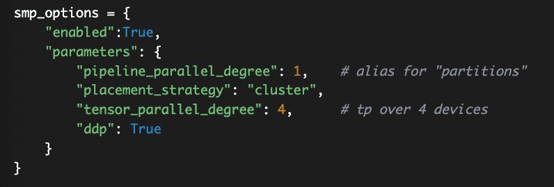
In the preceding code, pipeline_parallel_degree describes into how many segments your model should be sharded, based on the pipeline parallelism we discussed above. Another word for this is partitions.
To enable tensor parallelism, set tensor_parallel_degree to your desired level. Make sure you’re picking a number equal to or smaller than the number of GPU’s per instance, so no greater than 8 for the ml.p4d.24xlarge machines. For additional script changes, refer to Run a SageMaker Distributed Model Parallel Training Job with Tensor Parallelism.
The ddp parameter refers to distributed data parallel. You typically enable this if you’re using data parallelism or tensor parallelism, because the model parallelism library relies on DDP for these features.
Optimizer state sharding, activation offloading and checkpoints
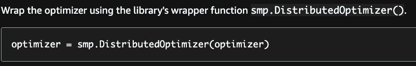
If you have an extremely large model, you also need an extremely large optimizer state. Prepping your optimizer for SMP is straightforward: simply pick it up from disk in your script and load it into the smp.DistributedOptimizer() object.
Make sure you enable this at the estimator by setting shard_optimizer_state to True in the smp_options you use to configure SMP:
![]()
Similar to tensor and pipeline parallelism, SMP profiles your model and your world size (the total number of GPUs in all of your training nodes), to find the best placement strategies.
In deep learning the intermediate layer outputs are also called activations, and these need to be stored during forward pass. This is because they need to be used for gradient computation in the backward pass. In a large model, storing all these activations simultaneously in memory can create significant memory bottlenecks. To address this bottleneck, you can use activation checkpointing, the third new feature in the SageMaker model parallelism library. Activation checkpointing, or gradient checkpointing, is a technique to reduce memory usage by clearing activations of certain layers and recomputing them during a backward pass. This effectively trades extra computation time for reduced memory usage.
Lastly, activation offloading directly uses activation checkpointing. It’s a strategy to keep only a few tensor activations on the GPU RAM during the model training. Specifically, we move the checkpointed activations to CPU memory during the forward pass and load them back to GPU for the backward pass of a specific micro-batch.
Micro-batches and placement strategies
Other topics that sometimes cause customers confusion are micro-batches and placement strategies. Both of these are hyperparameters you can supply to the SageMaker model parallel library. Specifically micro-batches are relevant when implementing models that rely on pipeline parallelism, such as those at least 30 billion parameters in size or more.
Micro-batches are subsets of minibatches. When your model is in its training loop, you define a certain number of records to pick up and pass forward and backward through the layers–this is called a minibatch, or sometimes just a batch. A full pass through your dataset is called an epoch. To run forward and backward passes with pipeline parallelism, SageMaker model parallel library shards the batches into smaller subsets called micro-batches, which are run one at a time to maximize GPU utilization. The resultant, much smaller set of examples per-GPU, is called a micro-batch. In our GPT-2 example, we added a default of 1 microbatch directly to the training script.
As you scale up your training configuration, you are strongly recommended to change your batch size and micro-batch size accordingly. This is the only way to ensure good performance: you must consider batch size and micro-batch sizes as a function of your overall world size when relying on pipeline parallelism.
Placement strategies are how to tell SageMaker physically where to place your model partitions. If you’re using both model parallel and data parallel, setting placement_strategy to “cluster” places model replicas in device ID’s (GPUs) that are physically close to each other. However, if you really want to be more prescriptive about your parallelism strategy, you can break it down into a single string with different combinations of three letters: D for data parallelism, P indicates pipeline parallelism, and T for tensor parallelism. We generally recommend keeping the default placement of "cluster", because this is most appropriate for large scale model training. The “cluster” placement corresponds to “DPT“.
For more information about placement strategies, see Placement Strategy with Tensor Parallelism.
Example use case
Let’s imagine you have one ml.p3.16xlarge in your training job. That gives you 8 NVIDIA V100’s per node. Remember, every time you add an extra instance, you experience additional bandwidth overhead, so it’s always better to have more GP’Us on a single node. In this case, you’re better off with one ml.p3.16xlarge than, for example, two ml.p3.8xlarges. Even though the number of GPUs is the same, the extra bandwidth overhead of the extra node slows down your throughput.
The following diagram illustrates four-way model parallelism, combined with two-way data parallelism. This means you actually have two replicas of your model (think data parallel), with each of them partitioned across four GPU’s (model parallel).
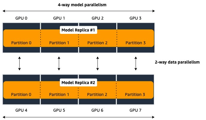
If any of those model partitions are too large to fit onto a single GPU, you can add an extra type of distribution–tensor parallelism–to spit it and utilize both devices.
Conclusion
In this blog post we discussed SageMaker distributed training libraries, especially focusing on model parallelism. We shared performance benchmarks from our latest test, achieving 32 samples per second across 120 ml.p4d.24xlarge instances and 175B parameters on Amazon SageMaker. We anticipate that if we increased this to 240 p4 instances we could train a 175B parameter model in 25 days.
We also discussed the newest features the enable large-scale training, namely tensor parallelism, optimizer state sharding, activation checkpointing, and activation offloading. We shared some tips and tricks for enabling this through training on Amazon SageMaker.
Try it out yourself using the same notebook that generated our numbers, which is available on GitHub here. You can also request more GPUs for your AWS account through requesting a service limit approval right here.
About the Authors
 Emily Webber joined AWS just after SageMaker launched, and has been trying to tell the world about it ever since! Outside of building new ML experiences for customers, Emily enjoys meditating and studying Tibetan Buddhism.
 Aditya Bindal is a Senior Product Manager for AWS Deep Learning. He works on products that make it easier for customers to train deep learning models on AWS. In his spare time, he enjoys spending time with his daughter, playing tennis, reading historical fiction, and traveling.
 Luis Quintela is the Software Developer Manager for the AWS SageMaker model parallel library. In his spare time, he can be found riding his Harley in the SF Bay Area.
ML inferencing at the edge with Amazon SageMaker Edge and Ambarella CV25
Ambarella builds computer vision SoCs (system on chips) based on a very efficient AI chip architecture and CVflow that provides the Deep Neural Network (DNN) processing required for edge inferencing use cases like intelligent home monitoring and smart surveillance cameras. Developers convert models trained with frameworks (such as TensorFlow or MXNET) to Ambarella CVflow format to be able to run these models on edge devices. Amazon SageMaker Edge has integrated the Ambarella toolchain into its workflow, allowing you to easily convert and optimize your models for the platform.
In this post, we show how to set up model optimization and conversion with SageMaker Edge, add the model to your edge application, and deploy and test your new model in an Ambarella CV25 device to build a smart surveillance camera application running on the edge.
Smart camera use case
Smart security cameras have use case-specific machine learning (ML) enabled features like detecting vehicles and animals, or identifying possible suspicious behavior, parking, or zone violations. These scenarios require ML models run on the edge computing unit in the camera with the highest possible performance.
Ambarella’s CVx processors, based on the company’s proprietary CVflow architecture, provide high DNN inference performance at very low power. This combination of high performance and low power makes them ideal for devices that require intelligence at the edge. ML models need to be optimized and compiled for the target platform to run on the edge. SageMaker Edge plays a key role in optimizing and converting ML models to the most popular frameworks to be able to run on the edge device.
Solution overview
Our smart security camera solution implements ML model optimization and compilation configuration, runtime operation, inference testing, and evaluation on the edge device. SageMaker Edge provides model optimization and conversion for edge devices to run faster with no loss in accuracy. The ML model can be in any framework that SageMaker Edge supports. For more information, see Supported Frameworks, Devices, Systems, and Architectures.
The SageMaker Edge integration of Ambarella CVflow tools provides additional advantages to developers using Ambarella SoCs:
- Developers don’t need to deal with updates and maintenance of the compiler toolchain, because the toolchain is integrated and opaque to the user
- Layers that CVflow doesn’t support are automatically compiled to run on the ARM by the SageMaker Edge compiler
The following diagram illustrates the solution architecture:
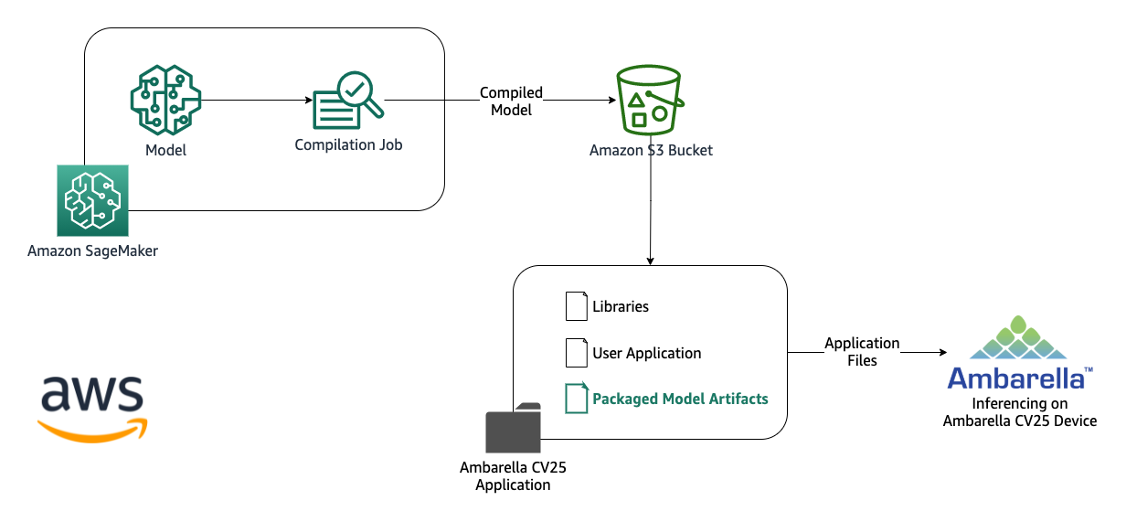
The steps to implement the solution are as follows:
- Prepare the model package.
- Configure and start the model’s compilation job for Ambarella CV25.
- Place the packaged model artifacts on the device.
- Test the inference on the device.
Prepare the model package
For Ambarella targets, SageMaker Edge requires a model package that contains a model configuration file called amba_config.json, calibration images, and a trained ML model file. This model package file is a compressed TAR file (*.tar.gz). You can use an Amazon Sagemaker notebook instance to train and test ML models and to prepare the model package file. To create a notebook instance, complete the following steps:
- On the SageMaker console, under Notebook in the navigation pane, choose Notebook instances.

- Choose Create notebook instance.
- Enter a name for your instance and choose ml.t2.medium as the instance type.
This instance is enough for testing and model preparation purposes.
- For IAM role, create a new AWS Identity and Access Management (IAM) role to allow access to Amazon Simple Storage Service (Amazon S3) buckets, or choose an existing role.
- Keep other configurations as default and choose Create notebook instance.
When the status is InService, you can start using your new Sagemaker notebook instance.
- Choose Open JupyterLab to access your workspace.
For this post, we use a pre-trained TFLite model to compile and deploy to the edge device. The chosen model is a pre-trained SSD object detection model from the TensorFlow model zoo on the COCO dataset.
- Download the converted TFLite model.
Now you’re ready to download, test, and prepare the model package.
- Create a new notebook with kernel
conda_tensorflow2_p36on the launcher view. - Import the required libraries as follows:
- Save the following example image as
street-frame.jpg, create a folder called calib_img in the workspace folder, and upload the image to the current folder. - Upload the downloaded model package contents to the current folder.

- Run the following command to load your pre-trained TFLite model and print its parameters, which we need to configure our model for compilation:
- Use following code to load the test image and run inference:
- Use the following code to visualize the detected bounding boxes on the image and save the result image as
street-frame_results.jpg: - Use following command to show the result image:
You get an inference result like the following image.

Our pre-trained TFLite model detects the car object from a security camera frame.
We’re done with testing the model; now let’s package the model and configuration files that Amazon Sagemaker Neo requires for Ambarella targets.
- Create an empty text file called
amba_config.jsonand use the following content for it:
This file is the compilation configuration file for Ambarella CV25. The filepath value inside amba_config.json should match the calib_img folder name; a mismatch may cause a failure.
The model package contents are now ready.
- Use the following commands to compress the package as a .tar.gz file:
- Upload the file to the SageMaker auto-created S3 bucket to use in the compilation job (or your designated S3 bucket):
The model package file contains calibration images, the compilation config file, and model files. After you upload the file to Amazon S3, you’re ready to start the compilation job.
Compile the model for Ambarella CV25
To start the compilation job, complete the following steps:
- On the SageMaker console, under Inference in the navigation pane, choose Compilation jobs.

- Choose Create compilation job.
- For Job name, enter a name.
- For IAM role, create a role or choose an existing role to give Amazon S3 read and write permission for the model files.

- In the Input configuration section, for Location of model artifacts, enter the S3 path of your uploaded model package file.
- For Data input configuration, enter
{"normalized_input_image_tensor":[1, 300, 300, 3]}, which is the model’s input data shape obtained in previous steps. - For Machine learning framework, choose TFLite.

- In the Output configuration section, for Target device, choose your device (
amba_cv25). - For S3 Output location, enter a folder in your S3 bucket for the compiled model to be saved in.
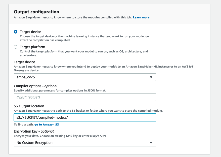
- Choose Submit to start the compilation process.
The compilation time depends on your model size and architecture. When your compiled model is ready in Amazon S3, the Status column shows as COMPLETED.
If the compilation status shows FAILED, refer to Troubleshoot Ambarella Errors to debug compilation errors.
Place the model artifacts on the device
When the compilation job is complete, Neo saves the compiled package to the provided output location in the S3 bucket. The compiled model package file contains the converted and optimized model files, their configuration, and runtime files.
On the Amazon S3 console, download the compiled model package, then extract and transfer the model artifacts to your device to start using it with your edge ML inferencing app.
Test the ML inference on the device
Navigate to your Ambarella device’s terminal and run the inferencing application binary on the device. The compiled and optimized ML model runs for the specified video source. You can observe detected bounding boxes on the output stream, as shown in the following screenshot.

Conclusion
In this post, we accomplished ML model preparation and conversion to Ambarella targets with SageMaker Edge, which has integrated the Ambarella toolchain. Optimizing and deploying high-performance ML models to Ambarella’s low-power edge devices unlocks intelligent edge solutions like smart security cameras.
As a next step, you can get started with SageMaker Edge and Ambarella CV25 to enable ML for edge devices. You can extend this use case with Sagemaker ML development features to build an end-to-end pipeline that includes edge processing and deployment.
About the Authors
 Emir Ayar is an Edge Prototyping Lead Architect on the AWS Prototyping team. He specializes in helping customers build IoT, Edge AI, and Industry 4.0 solutions and implement architectural best practices. He lives in Luxembourg and enjoys playing synthesizers.
 Dinesh Balasubramaniam is responsible for marketing and customer support for Ambarella’s family of security SoCs, with expertise in systems engineering, software development, video compression, and product design. Dinesh He earned an MS EE degree from the University of Texas at Dallas with a focus on signal processing.
Anomaly detection with Amazon SageMaker Edge Manager using AWS IoT Greengrass V2
Deploying and managing machine learning (ML) models at the edge requires a different set of tools and skillsets as compared to the cloud. This is primarily due to the hardware, software, and networking restrictions at the edge sites. This makes deploying and managing these models more complex. An increasing number of applications, such as industrial automation, autonomous vehicles, and automated checkouts, require ML models that run on devices at the edge so predictions can be made in real time when new data is available.
Another common challenge you may face when dealing with computing applications at the edge is how to efficiently manage the fleet of devices at scale. This includes installing applications, deploying application updates, deploying new configurations, monitoring device performance, troubleshooting devices, authenticating and authorizing devices, and securing the data transmission. These are foundational features for any edge application, but creating the infrastructure needed to achieve a secure and scalable solution requires a lot of effort and time.
On a smaller scale, you can adopt solutions such as manually logging in to each device to run scripts, use automated solutions such as Ansible, or build custom applications that rely on services such as AWS IoT Core. Although it can provide the necessary scalability and reliability, building such custom solutions comes at the cost of additional maintenance and requires specialized skills.
Amazon SageMaker, together with AWS IoT Greengrass, can help you overcome these challenges.
SageMaker provides Amazon SageMaker Neo, which is the easiest way to optimize ML models for edge devices, enabling you to train ML models one time in the cloud and run them on any device. As devices proliferate, you may have thousands of deployed models running across your fleets. Amazon SageMaker Edge Manager allows you to optimize, secure, monitor, and maintain ML models on fleets of smart cameras, robots, personal computers, and mobile devices.
This post shows how to train and deploy an anomaly detection ML model to a simulated fleet of wind turbines at the edge using features of SageMaker and AWS IoT Greengrass V2. It takes inspiration from Monitor and Manage Anomaly Detection Models on a fleet of Wind Turbines with Amazon SageMaker Edge Manager by introducing AWS IoT Greengrass for deploying and managing inference application and the model on the edge devices.
In the previous post, the author used custom code relying on AWS IoT services, such as AWS IoT Core and AWS IoT Device Management, to provide the remote management capabilities to the fleet of devices. Although that is a valid approach, developers need to spend a lot of time and effort to implement and maintain such solutions, which they could spend on solving the business problem of providing efficient, performant, and accurate anomaly detection logic for the wind turbines.
The previous post also used a real 3D printed mini wind turbine and Jetson Nano to act as the edge device running the application. Here, we use virtual wind turbines that run as Python threads within a SageMaker notebook. Also, instead of Jetson Nano, we use Amazon Elastic Compute Cloud (Amazon EC2) instances to act as edge devices, running AWS IoT Greengrass software and the application. We also run a simulator to generate measurements for the wind turbines, which are sent to the edge devices using MQTT. We also use the simulator for visualizations and stopping or starting the turbines.
The previous post goes more in detail about the ML aspects of the solution, such as how to build and train the model, which we don’t cover here. We focus primarily on the integration of Edge Manager and AWS IoT Greengrass V2.
Before we go any further, let’s review what AWS IoT Greengrass is and the benefits of using it with Edge Manager.
What is AWS IoT Greengrass V2?
AWS IoT Greengrass is an Internet of Things (IoT) open-source edge runtime and cloud service that helps build, deploy, and manage device software. You can use AWS IoT Greengrass for your IoT applications on millions of devices in homes, factories, vehicles, and businesses. AWS IoT Greengrass V2 offers an open-source edge runtime, improved modularity, new local development tools, and improved fleet deployment features. It provides a component framework that manages dependencies, and allows you to reduce the size of deployments because you can choose to only deploy the components required for the application.
Let’s go through some of the concepts of AWS IoT Greengrass to understand how it works:
- AWS IoT Greengrass core device – A device that runs the AWS IoT Greengrass Core software. The device is registered into the AWS IoT Core registry as an AWS IoT thing.
- AWS IoT Greengrass component – A software module that is deployed to and runs on a core device. All software that is developed and deployed with AWS IoT Greengrass is modeled as a component.
- Deployment – The process to send components and apply the desired component configuration to a destination target device, which can be a single core device or a group of core devices.
- AWS IoT Greengrass core software – The set of all AWS IoT Greengrass software that you install on a core device.
To enable remote application management on a device (or thousands of them), we first install the core software. This software runs as a background process and listens to deployments configurations sent from the cloud.
To run specific applications on the devices, we model the application as one or more components. For example, we can have a component providing a database feature, another component providing a local UX, or we can use public components provided by AWS, such as LogManager to push the components logs to Amazon CloudWatch.
We then create a deployment containing the necessary components and their specific configuration and send it to the target devices, either on a device-by-device basis or as a fleet.
To learn more, refer to What is AWS IoT Greengrass?
Why use AWS IoT Greengrass with Edge Manager?
The post Monitor and Manage Anomaly Detection Models on a fleet of Wind Turbines with Amazon SageMaker Edge Manager already explains why we use Edge Manager to provide the ML model runtime for the application. But let’s understand why we should use AWS IoT Greengrass to deploy applications to edge devices:
- With AWS IoT Greengrass, you can automate the tasks needed to deploy the Edge Manager software onto the devices and manage the ML models. AWS IoT Greengrass provides a SageMaker Edge Agent as an AWS IoT Greengrass component, which provides model management and data capture APIs on the edge. Without AWS IoT Greengrass, setting up devices and fleets to use Edge Manager requires you to manually copy the Edge Manager agent from an Amazon Simple Storage Service (Amazon S3) release bucket. The agent is used to make predictions with models loaded onto edge devices.
- With AWS IoT Greengrass and Edge Manager integration, you use AWS IoT Greengrass components. Components are pre-built software modules that can connect edge devices to AWS services or third-party services via AWS IoT Greengrass.
- The solution takes a modular approach in which the inference application, model, and any other business logic can be packaged as a component where the dependencies can also be specified. You can manage the lifecycle, updates, and reinstalls of each of the components independently rather than treat everything as a monolith.
- To make it easier to maintain AWS Identity and Access Management (IAM) roles, Edge Manager allows you to reuse the existing AWS IoT Core role alias. If it doesn’t exist, Edge Manager generates a role alias as part of the Edge Manager packaging job. You no longer need to associate a role alias generated from the Edge Manager packaging job with an AWS IoT Core role. This simplifies the deployment process for existing AWS IoT Greengrass customers.
- You can manage the models and other components with less code and configurations because AWS IoT Greengrass takes care of provisioning, updating, and stopping the components.
Solution overview
The following diagram is the architecture implemented for the solution:
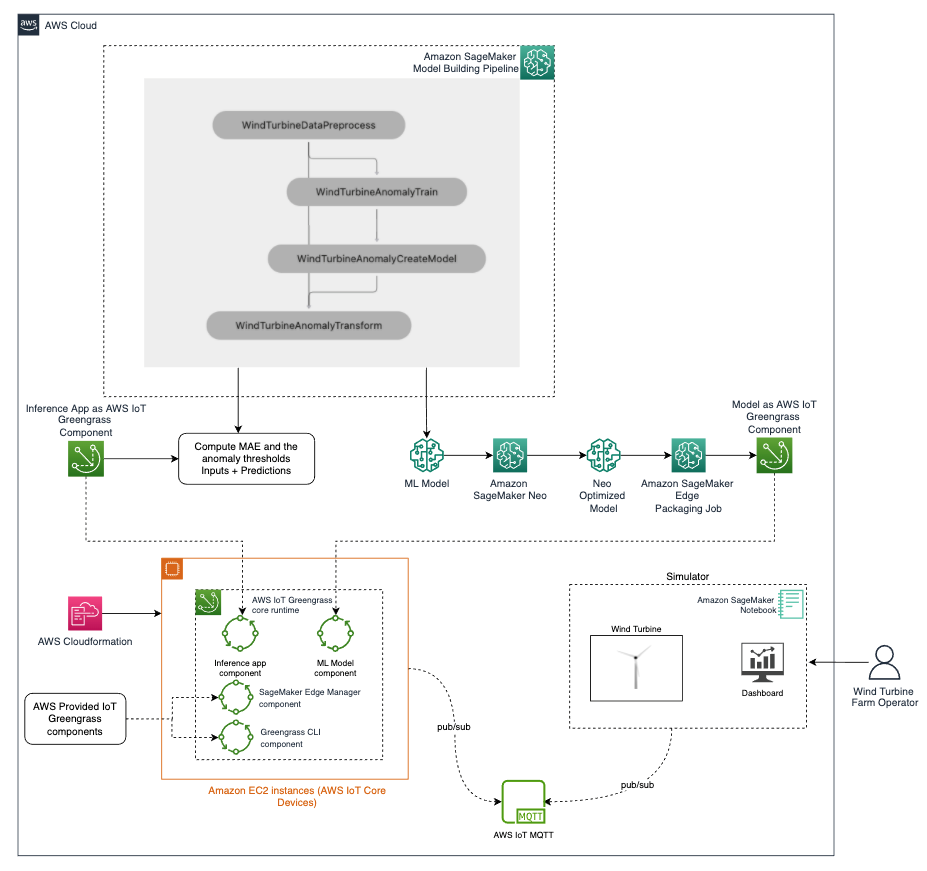
We can broadly divide the architecture into the following phases:
-
Model training
- Prepare the data and train an anomaly detection model using Amazon SageMaker Pipelines. SageMaker Pipelines helps orchestrate your training pipeline with your own custom code. It also outputs the Mean Absolute Error (MAE) and other threshold values used to calculate anomalies.
-
Compile and package the model
- Compile the model using Neo, so that it can be optimized for the target hardware (in this case, an EC2 instance).
- Use the SageMaker Edge packaging job API to package the model as an AWS IoT Greengrass component. The Edge Manager API has a native integration with AWS IoT Greengrass APIs.
-
Build and package the inference application
- Build and package the inference application as an AWS IoT Greengrass component. This application uses the computed threshold, the model, and some custom code to accept the data coming from turbines, perform anomaly detection, and return results.
-
Set up AWS IoT Greengrass on edge devices
- Set up a fleet of AWS IoT Greengrass core devices. In this architecture, we use EC2 instances to act as core devices. We spin up five EC2 instances via AWS CloudFormation and install the AWS IoT Greengrass core runtime on those instances.
-
Deploy to edge devices
- Deploy the following on each edge device:
- An ML model packaged as an AWS IoT Greengrass component.
- An inference application packaged an AWS IoT Greengrass component. This also sets up the connection to AWS IoT Core MQTT.
- The AWS-provided Edge Manager Greengrass component.
- The AWS-provided AWS IoT Greengrass CLI component (only needed for development and debugging purposes).
- Deploy the following on each edge device:
-
Run the end-to-end solution
- Run the simulator, which generates measurements for the wind turbines, which are sent to the edge devices using MQTT.
- Because the notebook and the EC2 instances running AWS IoT Greengrass are on different networks, we use AWS IoT Core to relay MQTT messages between them. In a real scenario, the wind turbine would send the data to the anomaly detection device using a local communication, for example, an AWS IoT Greengrass MQTT broker component.
- The inference app and model running in the anomaly detection device predicts if the received data is anomalous or not, and sends the result to the monitoring application via MQTT through AWS IoT Core.
- The application displays the data and anomaly signal on the simulator dashboard.
To know more on how to deploy this solution architecture, please refer to the GitHub Repository related to this post.
In the following sections, we go deeper into the details of how to implement this solution.
Dataset
The solution uses raw turbine data collected from real wind turbines. The dataset is provided as part of the solution. It has the following features:
- nanoId – ID of the edge device that collected the data
- turbineId – ID of the turbine that produced this data
- arduino_timestamp – Timestamp of the Arduino that was operating this turbine
- nanoFreemem: Amount of free memory in bytes
- eventTime – Timestamp of the row
- rps – Rotation of the rotor in rotations per second
- voltage – Voltage produced by the generator in milivolts
- qw, qx, qy, qz – Quaternion angular acceleration
- gx, gy, gz – Gravity acceleration
- ax, ay, az – Linear acceleration
- gearboxtemp – Internal temperature
- ambtemp – External temperature
- humidity – Air humidity
- pressure – Air pressure
- gas – Air quality
- wind_speed_rps – Wind speed in rotations per second
For more information, refer to Monitor and Manage Anomaly Detection Models on a fleet of Wind Turbines with Amazon SageMaker Edge Manager.
Data preparation and training
The data preparation and training are performed using SageMaker Pipelines. Pipelines is the first purpose-built, easy-to-use continuous integration and continuous delivery (CI/CD) service for ML. With Pipelines, you can create, automate, and manage end-to-end ML workflows at scale. Because it’s purpose-built for ML, Pipelines helps automate different steps of the ML workflow, including data loading, data transformation, training and tuning, and deployment. For more information, refer to Amazon SageMaker Model Building Pipelines.
Model compilation
We use Neo for model compilation. It automatically optimizes ML models for inference on cloud instances and edge devices to run faster with no loss in accuracy. ML models are optimized for a target hardware platform, which can be a SageMaker hosting instance or an edge device based on processor type and capabilities, for example if there is a GPU or not. The compiler uses ML to apply the performance optimizations that extract the best available performance for your model on the cloud instance or edge device. For more information, see Compile and Deploy Models with Neo.
Model packaging
To use a compiled model with Edge Manager, you first need to package it. In this step, SageMaker creates an archive consisting of the compiled model and the Neo DLR runtime required to run it. It also signs the model for integrity verification. When you deploy the model via AWS IoT Greengrass, the create_edge_packaging_job API automatically creates an AWS IoT Greengrass component containing the model package, which is ready to be deployed to the devices.
The following code snippet shows how to invoke this API:
To allow the API to create an AWS IoT Greengrass component, you must provide the following additional parameters under OutputConfig:
- The
PresetDeploymentTypeasGreengrassV2Component -
PresetDeploymentConfigto provide theComponentNameandComponentVersionthat AWS IoT Greengrass uses to publish the component - The
ComponentVersionandModelVersionmust be inmajor.minor.patchformat
The model is then published as an AWS IoT Greengrass component.
Create the inference application as an AWS IoT Greengrass component
Now we create an inference application component that we can deploy to the device. This application component loads the ML model, receives data from wind turbines, performs anomaly detections, and sends the result back to the simulator. This application can be a native application that receives the data locally on the edge devices from the turbines or any other client application over a gRPC interface.
To create a custom AWS IoT Greengrass component, perform the following steps:
- Provide the code for the application as single files or as an archive. The code needs to be uploaded to an S3 bucket in the same Region where we registered the AWS IoT Greengrass devices.
- Create a recipe file, which specifies the component’s configuration parameters, component dependencies, lifecycle, and platform compatibility.
The component lifecycle defines the commands that install, run, and shut down the component. For more information, see AWS IoT Greengrass component recipe reference. We can define the recipe either in JSON or YAML format. Because the inference application requires the model and Edge Manager agent to be available on the device, we need to specify dependencies to the ML model packaged as an AWS IoT Greengrass component and the Edge Manager Greengrass component.
- When the recipe file is ready, create the inference component by invoking the create_component_version API. See the following code:
Inference application
The inference application connects to AWS IoT Core to receive messages from the simulated wind turbine and send the prediction results to the simulator dashboard.
It publishes to the following topics:
-
wind-turbine/{turbine_id}/dashboard/update– Updates the simulator dashboard -
wind-turbine/{turbine_id}/label/update– Updates the model loaded status on simulator -
wind-turbine/{turbine_id}/anomalies– Publishes anomaly results to the simulator dashboard
It subscribes to the following topic:
-
wind-turbine/{turbine_id}/raw-data– Receives raw data from the turbine
Set up AWS IoT Core devices
Next, we need to set up the devices that run the anomaly detection application by installing the AWS IoT Greengrass core software. For this post, we use five EC2 instances that act as the anomaly detection devices. We use AWS CloudFormation to launch the instances. To install the AWS IoT Greengrass core software, we provide a script in the instance UserData as shown in the following code:
Each EC2 instance is associated to a single virtual wind turbine. In a real scenario, multiple wind turbines could also communicate to a single device in order to reduce the solution costs.
To learn more about how to set up AWS IoT Greengrass software on a core device, refer to Install the AWS IoT Greengrass Core software. The complete CloudFormation template is available in the GitHub repository.
Create an AWS IoT Greengrass deployment
When the devices are up and running, we can deploy the application. We create a deployment with a configuration containing the following components:
- ML model
- Inference application
- Edge Manager
- AWS IoT Greengrass CLI (only needed for debugging purposes)
For each component, we must specify the component version. We can also provide additional configuration data, if necessary. We create the deployment by invoking the create_deployment API. See the following code:
The targetArn argument defines where to run the deployment. The thing group ARN is specified to deploy this configuration to all devices belonging to the thing group. The thing group is created already as part of the setup of the solution architecture.
The aws.greengrass.SageMakerEdgeManager component is an AWS-provided component by AWS IoT Greengrass. At the time of writing, the latest version is 1.1.0. You need to configure this component with the SageMaker edge device fleet name and S3 bucket location. You can find these parameters on the Edge Manager console, where the fleet was created during the setup of the solution architecture.
aws.samples.windturbine.detector is the inference application component created earlier.
aws.samples.windturbine.model is the anomaly detection ML model component created earlier.
Run the simulator
Now that everything is in place, we can start the simulator. The simulator is run from a Python notebook and performs two tasks:
- Simulate the physical wind turbine and display a dashboard for each wind turbine.
- Exchange data with the devices via AWS IoT MQTT using the following topics:
-
wind-turbine/{turbine_id}/raw-data– Publishes the raw turbine data. -
wind-turbine/{turbine_id}/label/update– Receives model loaded or not loaded status from the inference application. -
wind-turbine/{turbine_id}/anomalies– Receives anomalies published by inference application. -
wind-turbine/{turbine_id}/dashboard/update– Receives recent buffered data by the turbines.
-
We can use the simulator UI to start and stop the virtual wind turbine and inject noise in the Volt, Rot, and Vib measurements to simulate anomalies that are detected by the application running on the device. In the following screenshot, the simulator shows a virtual representation of five wind turbines that are currently running. We can choose Stop to stop any of the turbines, or choose Volt, Rot, or Vib to inject noise in the turbines. For example, if we choose Volt for turbine with ID 0, the Voltage status changes from a green check mark to a red x, denoting the voltage readings of the turbine are anomalous.
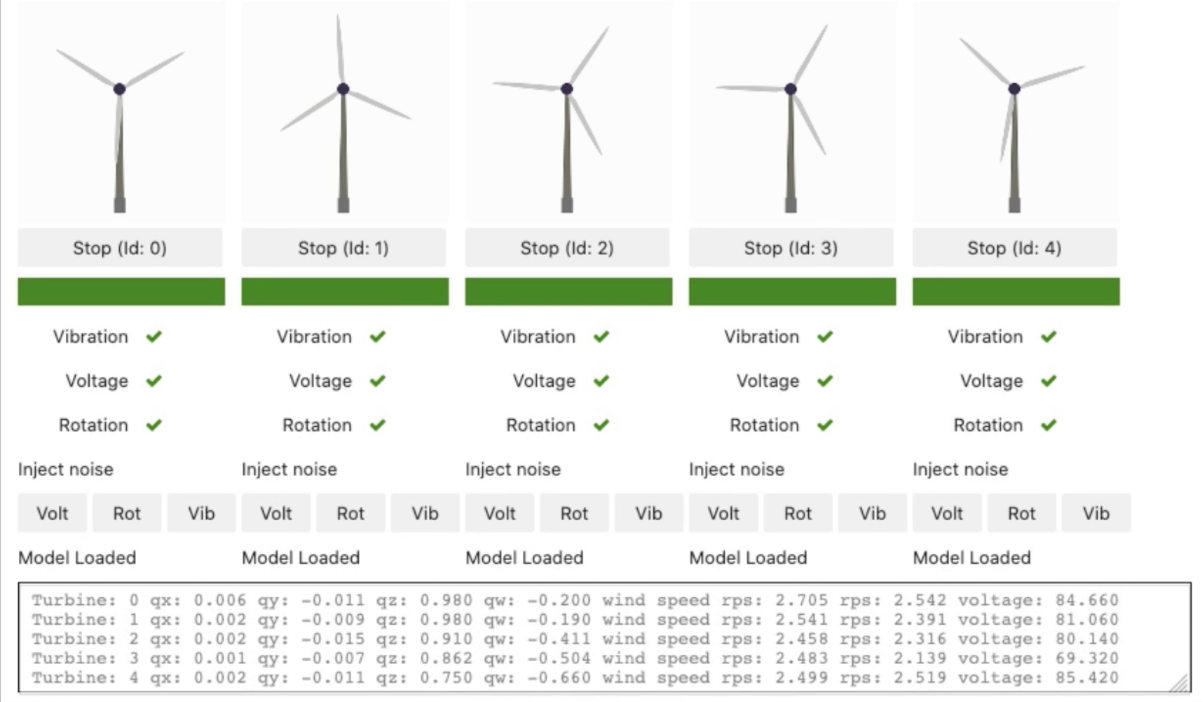
Conclusion
Securely and reliably maintaining the lifecycle of an ML model deployed across a fleet of devices isn’t an easy task. However, with Edge Manager and AWS IoT Greengrass, we can reduce the implementation effort and operational cost of such a solution. This solution increases the agility in experimenting and optimizing the ML model with full automation of the ML pipelines, from data acquisition, data preparation, model training, model validation, and deployment to the devices.
In addition to the benefits described, Edge Manager offers further benefits, like having access to a device fleet dashboard on the Edge Manager console, which can display near-real-time health of the devices by capturing heartbeat requests. You can use this inference data with Amazon SageMaker Model Monitor to check for data and model quality drift issues.
To build a solution for your own needs, get the code and artifacts from the GitHub repo. The repository shows two different ways of deploying the models:
- Using IoT jobs
- Using AWS IoT Greengrass (covered in this post)
Although this post focuses on deployment using AWS IoT Greengrass, interested readers look at the solution using IoT jobs as well to better understand the differences.
About the Authors
 Vikesh Pandey is a Machine Learning Specialist Specialist Solutions Architect at AWS, helping customers in the Nordics and wider EMEA region design and build ML solutions. Outside of work, Vikesh enjoys trying out different cuisines and playing outdoor sports.
 Massimiliano Angelino is Lead Architect for the EMEA Prototyping team. During the last 3 and half years he has been an IoT Specialist Solution Architect with a particular focus on edge computing, and he contributed to the launch of AWS IoT Greengrass v2 service and its integration with Amazon SageMaker Edge Manager. Based in Stockholm, he enjoys skating on frozen lakes.
How Haluk Demirkan is using machine learning to get devices to the right place at the right time
Part-time sabbatical plan turns into full-time role for author of five books and more than 170 research articles.Read More
Improving question-answering models that use data from tables
Novel pretraining method enables increases of 5% to 14% on five different evaluation metrics.Read More