Your contact center connects your business to your community, enabling customers to order products, callers to request support, clients to make appointments, and much more. When calls go well, callers retain a positive image of your brand, and are likely to return and recommend you to others. And the converse, of course, is also true.
Naturally, you want to do what you can to ensure that your callers have a good experience. There are two aspects to this:
- Help supervisors assess the quality of your caller’s experiences in real time – For example, your supervisors need to know if initially unhappy callers become happier as the call progresses. And if not, why? What actions can be taken, before the call ends, to assist the agent to improve the customer experience for calls that aren’t going well?
- Help agents optimize the quality of your caller’s experiences – For example, can you deploy live call transcription? This removes the need for your agents to take notes during calls, freeing them to focus more attention on providing positive customer interactions.
Contact Lens for Amazon Connect provides real-time supervisor and agent assist features that could be just what you need, but you may not yet be using Amazon Connect. You need a solution that works with your existing contact center.
Amazon Machine Learning (ML) services like Amazon Transcribe and Amazon Comprehend provide feature-rich APIs that you can use to transcribe and extract insights from your contact center audio at scale. Although you could build your own custom call analytics solution using these services, that requires time and resources. In this post, we introduce our new sample solution for live call analytics.
Solution overview
Our new sample solution, Live Call Analytics (LCA), does most of the heavy lifting associated with providing an end-to-end solution that can plug into your contact center and provide the intelligent insights that you need.
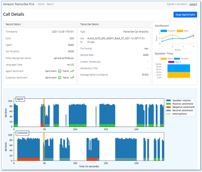
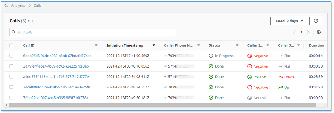
It has a call summary user interface, as shown in the following screenshot.
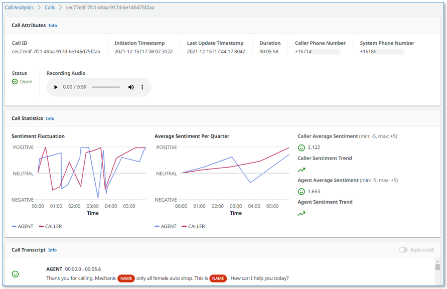
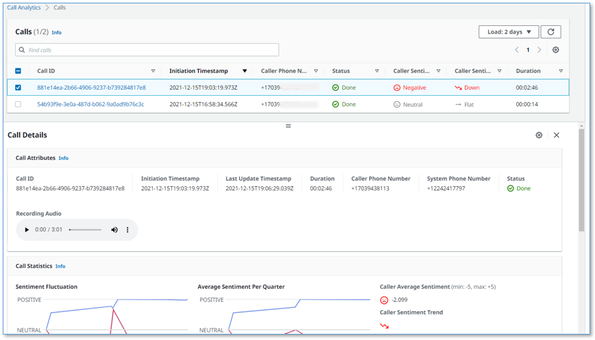
It also has a call detail user interface.
LCA currently supports the following features:
- Accurate streaming transcription with support for personally identifiable information (PII) redaction and custom vocabulary
- Sentiment detection
- Automatic scaling to handle call volume changes
- Call recording and archiving
- A dynamically updated web user interface for supervisors and agents:
- A call summary page that displays a list of in-progress and completed calls, with call timestamps, metadata, and summary statistics like duration, and sentiment trend
- Call detail pages showing live turn-by-turn transcription of the caller/agent dialog, turn-by-turn sentiment, and sentiment trend
- Standards-based telephony integration with your contact center using Session Recording Protocol (SIPREC)
- A built-in standalone demo mode that allows you to quickly install and try out LCA for yourself, without needing to integrate with your contact center telephony
- Easy-to-install resources with a single AWS CloudFormation template
This is just the beginning! We expect to add many more exciting features over time, based on your feedback.
Deploy the CloudFormation stack
Start your LCA experience by using AWS CloudFormation to deploy the sample solution with the built-in demo mode enabled.
The demo mode downloads, builds, and installs a small virtual PBX server on an Amazon Elastic Compute Cloud (Amazon EC2) instance in your AWS account (using the free open-source Asterisk project) so you can make test phone calls right away and see the solution in action. You can integrate it with your contact center later after evaluating the solution’s functionality for your unique use case.
- Use the appropriate Launch Stack button for the AWS Region in which you’ll use the solution. We expect to add support for additional Regions over time.
- US East (N. Virginia) us-east-1

- US West (Oregon) us-west-2
- US East (N. Virginia) us-east-1
- For Stack name, use the default value,
LiveCallAnalytics. - For Install Demo Asterisk Server, use the default value,
true. - For Allowed CIDR Block for Demo Softphone, use the IP address of your local computer with a network mask of
/32.
To find your computer’s IP address, you can use the website checkip.amazonaws.com.
Later, you can optionally install a softphone application on your computer, which you can register with LCA’s demo Asterisk server. This allows you to experiment with LCA using real two-way phone calls.
If that seems like too much hassle, don’t worry! Simply leave the default value for this parameter and elect not to register a softphone later. You will still be able to test the solution. When the demo Asterisk server doesn’t detect a registered softphone, it automatically simulates the agent side of the conversation using a built-in audio recording.
- For Allowed CIDR List for SIPREC Integration, leave the default value.
This parameter isn’t used for demo mode installation. Later, when you want to integrate LCA with your contact center audio stream, you use this parameter to specify the IP address of your SIPREC source hosts, such as your Session Border Controller (SBC) servers.
- For Authorized Account Email Domain, use the domain name part of your corporate email address (this allows others with email addresses in the same domain to sign up for access to the UI).
- For Call Audio Recordings Bucket Name, leave the value blank to have an Amazon Simple Storage Service (Amazon S3) bucket for your call recordings automatically created for you. Otherwise, use the name of an existing S3 bucket where you want your recordings to be stored.
- For all other parameters, use the default values.
If you want to customize the settings later, for example to apply PII redaction or custom vocabulary to improve accuracy, you can update the stack for these parameters.
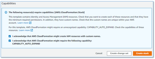
- Check the two acknowledgement boxes, and choose Create stack.

The main CloudFormation stack uses nested stacks to create the following resources in your AWS account:
- S3 buckets to hold build artifacts and call recordings
- An EC2 instance (t4g.large) with the demo Asterisk server installed, with VPC, security group, Elastic IP address, and internet gateway
- An Amazon Chime Voice Connector, configured to stream audio to Amazon Kinesis Video Streams
- An Amazon Elastic Container Service (Amazon ECS) instance that runs containers in AWS Fargate to relay streaming audio from Kinesis Video Streams to Amazon Transcribe and record transcription segments in Amazon DynamoDB, with VPC, NAT gateways, Elastic IP addresses, and internet gateway
- An AWS Lambda function to create and store final stereo call recordings
- A DynamoDB table to store call and transcription data, with Lambda stream processing that adds analytics to the live call data
- The AWS AppSync API, which provides a GraphQL endpoint to support queries and real-time updates
- Website components including S3 bucket, Amazon CloudFront distribution, and Amazon Cognito user pool
- Other miscellaneous supporting resources, including AWS Identity and Access Management (IAM) roles and policies (using least privilege best practices), Amazon Virtual Private Cloud (Amazon VPC) resources, Amazon EventBridge event rules, and Amazon CloudWatch log groups.
The stacks take about 20 minutes to deploy. The main stack status shows CREATE_COMPLETE when everything is deployed.

Create a user account
We now open the web user interface and create a user account.
- On the AWS CloudFormation console, choose the main stack,
LiveCallAnalytics, and choose the Outputs tab.
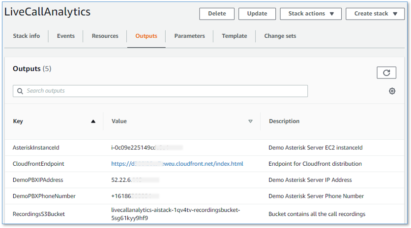
- Open your web browser to the URL shown as
CloudfrontEndpointin the outputs.
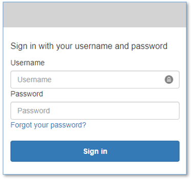
You’re directed to the login page.
- Choose Create account.
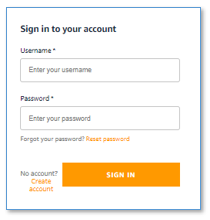
- For Username, use your email address that belongs to the email address domain you provided earlier.
- For Password, use a sequence that has a length of at least 8 characters, and contains uppercase and lowercase characters, plus numbers and special characters.
- Choose CREATE ACCOUNT.
The Confirm Sign up page appears.
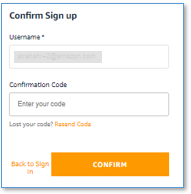
Your confirmation code has been emailed to the email address you used as your username. Check your inbox for an email from no-reply@verificationemail.com with subject “Account Verification.”
- For Confirmation Code, copy and paste the code from the email.
- Choose CONFIRM.
You’re now logged in to LCA.
Make a test phone call
Call the number shown as DemoPBXPhoneNumber in the AWS CloudFormation outputs for the main LiveCallAnalytics stack.
You haven’t yet registered a softphone app, so the demo Asterisk server picks up the call and plays a recording. Listen to the recording, and answer the questions when prompted. Your call is streamed to the LCA application, and is recorded, transcribed, and analyzed. When you log in to the UI later, you can see a record of this call.
Optional: Install and register a softphone
If you want to use LCA with live two-person phone calls instead of the demo recording, you can register a softphone application with your new demo Asterisk server.
The following README has step-by-step instructions for downloading, installing, and registering a free (for non-commercial use) softphone on your local computer. The registration is successful only if Allowed CIDR Block for Demo Softphone correctly reflects your local machine’s IP address. If you got it wrong, or if your IP address has changed, you can choose the LiveCallAnalytics stack in AWS CloudFormation, and choose Update to provide a new value for Allowed CIDR Block for Demo Softphone.
If you still can’t successfully register your softphone, and you are connected to a VPN, disconnect and update Allowed CIDR Block for Demo Softphone—corporate VPNs can restrict IP voice traffic.
When your softphone is registered, call the phone number again. Now, instead of playing the default recording, the demo Asterisk server causes your softphone to ring. Answer the call on the softphone, and have a two-way conversation with yourself! Better yet, ask a friend to call your Asterisk phone number, so you can simulate a contact center call by role playing as caller and agent.
Explore live call analysis features
Now, with LCA successfully installed in demo mode, you’re ready to explore the call analysis features.
- Open the LCA web UI using the URL shown as
CloudfrontEndpointin the main stack outputs.
We suggest bookmarking this URL—you’ll use it often!
- Make a test phone call to the demo Asterisk server (as you did earlier).
- If you registered a softphone, it rings on your local computer. Answer the call, or better, have someone else answer it, and use the softphone to play the agent role in the conversation.
- If you didn’t register a softphone, the Asterisk server demo audio plays the role of agent.
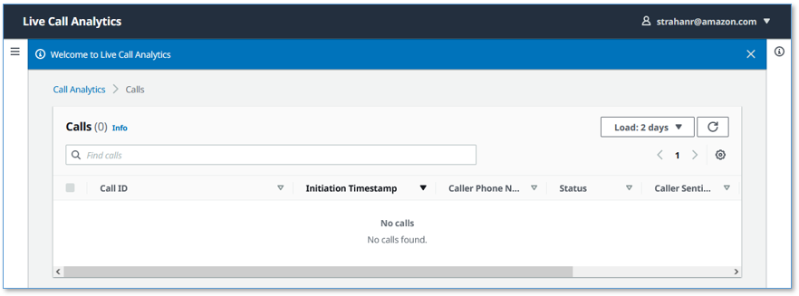
Your phone call almost immediately shows up at the top of the call list on the UI, with the status In progress.
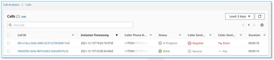
The call has the following details:
- Call ID – A unique identifier for this telephone call
- Initiation Timestamp – Shows the time the telephone call started
- Caller Phone Number – Shows the number of the phone from which you made the call
- Status – Indicates that the call is in progress
- Caller Sentiment – The average caller sentiment
- Caller Sentiment Trend –The caller sentiment trend
- Duration – The elapsed time since the start of the call
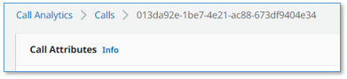
- Choose the call ID of your
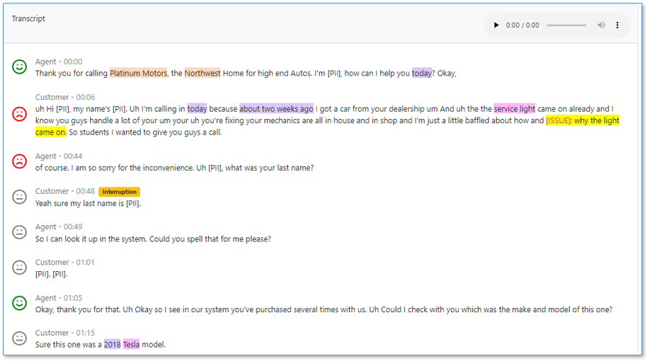
In progresscall to open the live call detail page.

As you talk on the phone from which you made the call, your voice and the voice of the agent are transcribed in real time and displayed in the auto scrolling Call Transcript pane.
Each turn of the conversation (customer and agent) is annotated with a sentiment indicator. As the call continues, the sentiment for both caller and agent is aggregated over a rolling time window, so it’s easy to see if sentiment is trending in a positive or negative direction.
- End the call.
- Navigate back to the call list page by choosing Calls at the top of the page.
Your call is now displayed in the list with the status Done.
- To display call details for any call, choose the call ID to open the details page, or select the call to display the Calls list and Call Details pane on the same page.
You can change the orientation to a side-by-side layout using the Call Details settings tool (gear icon).
You can make a few more phone calls to become familiar with how the application works. With the softphone installed, ask someone else to call your Asterisk demo server phone number: pick up their call on your softphone and talk with them while watching the turn-by-turn transcription update in real time. Observe the low latency. Assess the accuracy of transcriptions and sentiment annotation—you’ll likely find that it’s not perfect, but it’s close! Transcriptions are less accurate when you use technical or domain-specific jargon, but you can use custom vocabulary to teach Amazon Transcribe new words and terms.
Processing flow overview
How did LCA transcribe and analyze your test phone calls? Let’s take a quick look at how it works.
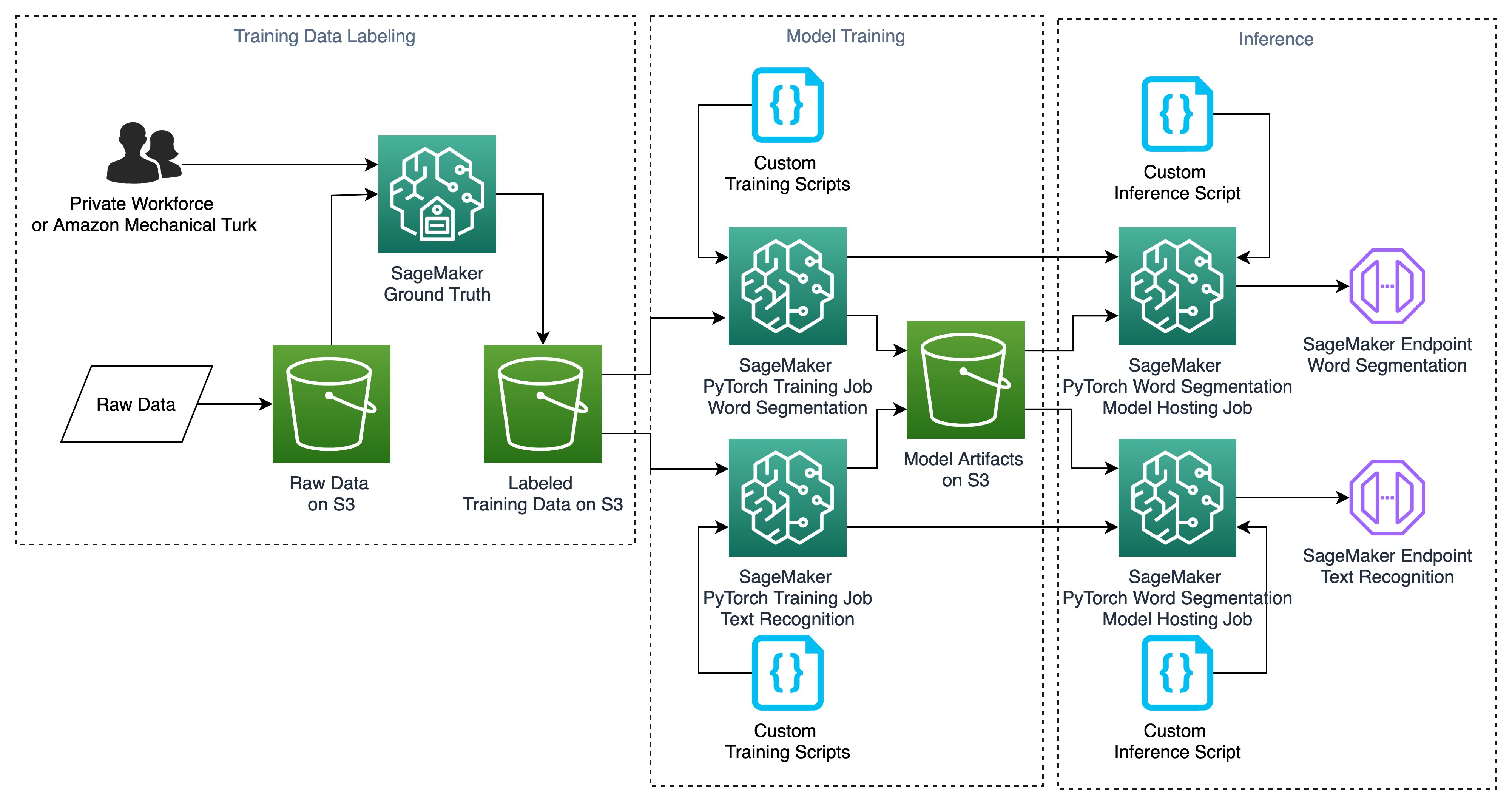
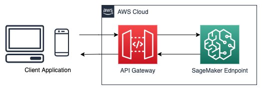
The following diagram shows the main architectural components and how they fit together at a high level.

The demo Asterisk server is configured to use Voice Connector, which provides the phone number and SIP trunking needed to route inbound and outbound calls. When you configure LCA to integrate with your contact center instead of the demo Asterisk server, Voice Connector is configured to integrate instead with your existing contact center using SIP-based media recording (SIPREC) or network-based recording (NBR). In both cases, Voice Connector streams audio to Kinesis Video Streams using two streams per call, one for the caller and one for the agent.
When a new video stream is initiated, an event is fired using EventBridge. This event triggers a Lambda function, which uses an Amazon Simple Queue Service (Amazon SQS) queue to initiate a new call processing job in Fargate, a serverless compute service for containers. A single container instance processes multiple calls simultaneously. AWS auto scaling provisions and de-provisions additional containers dynamically as needed to handle changing call volumes.
The Fargate container immediately creates a streaming connection with Amazon Transcribe and starts consuming and relaying audio fragments from Kinesis Video Streams to Amazon Transcribe.
The container writes the streaming transcription results in real time to a DynamoDB table.
A Lambda function, the Call Event Stream Processor, fed by DynamoDB streams, processes and enriches call metadata and transcription segments. The event processor function interfaces with AWS AppSync to persist changes (mutations) in DynamoDB and to send real-time updates to logged in web clients.
The LCA web UI assets are hosted on Amazon S3 and served via CloudFront. Authentication is provided by Amazon Cognito. In demo mode, user identities are configured in an Amazon Cognito user pool. In a production setting, you would likely configure Amazon Cognito to integrate with your existing identity provider (IdP) so authorized users can log in with their corporate credentials.
When the user is authenticated, the web application establishes a secure GraphQL connection to the AWS AppSync API, and subscribes to receive real-time events such as new calls and call status changes for the calls list page, and new or updated transcription segments and computed analytics for the call details page.
The entire processing flow, from ingested speech to live webpage updates, is event driven, and so the end-to-end latency is small—typically just a few seconds.
Monitoring and troubleshooting
AWS CloudFormation reports deployment failures and causes on the relevant stack Events tab. See Troubleshooting CloudFormation for help with common deployment problems. Look out for deployment failures caused by limit exceeded errors; the LCA stacks create resources such as NAT gateways, Elastic IP addresses, and other resources that are subject to default account and Region Service Quotas.
Amazon Transcribe has a default limit of 25 concurrent transcription streams, which limits LCA to 12 concurrent calls (two streams per call). Request an increase for the number of concurrent HTTP/2 streams for streaming transcription if you need to handle a larger number of concurrent calls.
LCA provides runtime monitoring and logs for each component using CloudWatch:
-
Call trigger Lambda function – On the Lambda console, open the
LiveCallAnalytics-AISTACK-transcribingFargateXXXfunction. Choose the Monitor tab to see function metrics. Choose View logs in CloudWatch to inspect function logs. -
Call processing Fargate task – On the Amazon ECS console, choose the
LiveCallAnalyticscluster. Open theLiveCallAnalyticsservice to see container health metrics. Choose the Logs tab to inspect container logs. -
Call Event Stream Processor Lambda function – On the Lambda console, open the
LiveCallAnalytics-AISTACK-CallEventStreamXXXfunction. Choose the Monitor tab to see function metrics. Choose View logs in CloudWatch to inspect function logs. -
AWS AppSync API – On the AWS AppSync console, open the
CallAnalytics-LiveCallAnalytics-XXXAPI. Choose Monitoring in the navigation pane to see API metrics. Choose View logs in CloudWatch to inspect AppSyncAPI logs.
Cost assessment
This solution has hourly cost components and usage cost components.
The hourly costs add up to about $0.15 per hour, or $0.22 per hour with the demo Asterisk server enabled. For more information about the services that incur an hourly cost, see AWS Fargate Pricing, Amazon VPC pricing (for the NAT gateway), and Amazon EC2 pricing (for the demo Asterisk server).
The hourly cost components comprise the following:
- Fargate container – 2vCPU at $0.08/hour and 4 GB memory at $0.02/hour = $0.10/hour
- NAT gateways – Two at $0.09/hour
- EC2 instance – t4g.large at $0.07/hour (for demo Asterisk server)
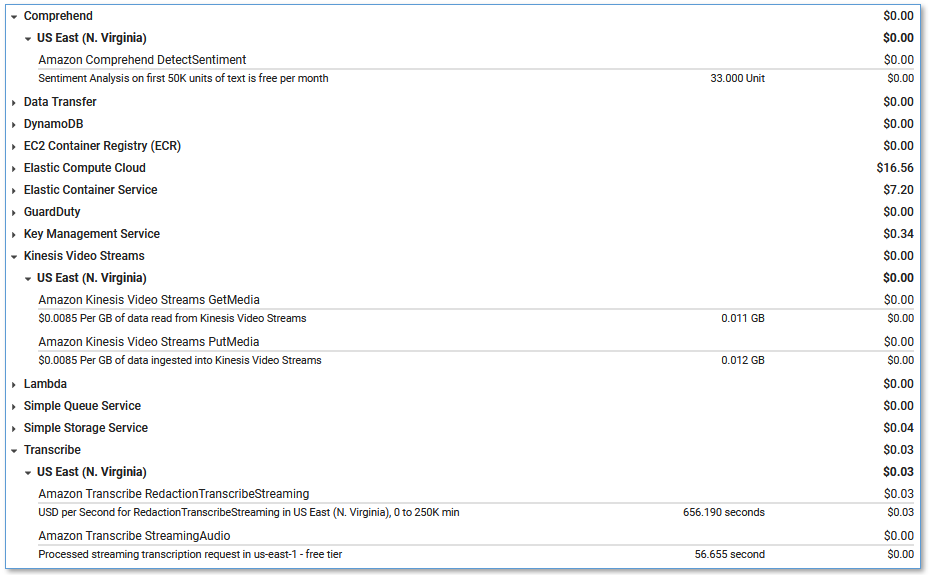
The usage costs add up to about $0.30 for a 5-minute call, although this can vary based on total usage, because usage affects Free Tier eligibility and volume tiered pricing for many services. For more information about the services that incur usage costs, see the following:
- AWS AppSync pricing
- Amazon Cognito Pricing
- Amazon Comprehend Pricing
- Amazon DynamoDB pricing
- Amazon EventBridge pricing
- Amazon Kinesis Video Streams pricing
- AWS Lambda Pricing
- Amazon SQS pricing
- Amazon S3 pricing
- Amazon Transcribe Pricing
- Amazon Voice Connector Chime pricing (streaming)
To explore LCA costs for yourself, use AWS Cost Explorer or choose Bill Details on the AWS Billing Dashboard to see your month-to-date spend by service.
Integrate with your contact center
To deploy LCA to analyze real calls to your contact center using AWS CloudFormation, update the existing LiveCallAnalytics demo stack, changing the parameters to disable demo mode.
Alternatively, delete the existing LiveCallAnalytics demo stack, and deploy a new LiveCallAnalytics stack (use the stack options from the previous section).
You could also deploy a new LiveCallAnalytics stack in a different AWS account or Region.
Use these parameters to configure LCA for contact center integration:
- For Install Demo Asterisk Server, enter
false. - For Allowed CIDR Block for Demo Softphone, leave the default value.
- For Allowed CIDR List for Siprec Integration, use the CIDR blocks of your SIPREC source hosts, such as your SBC servers. Use commas to separate CIDR blocks if you enter more than one.
When you deploy LCA, a Voice Connector is created for you. Use the Voice Connector documentation as guidance to configure this Voice Connector and your PBX/SBC for SIP-based media recording (SIPREC) or network-based recording (NBR). The Voice Connector Resources page provides some vendor-specific example configuration guides, including:
- SIPREC Configuration Guide: Cisco Unified Communications Manager (CUCM) and Cisco Unified Border Element (CUBE)
- SIPREC Configuration Guide: Avaya Aura Communication Manager and Session Manager with Sonus SBC 521
The LCA GitHub repository has additional vendor specific notes that you may find helpful; see SIPREC.md.
Customize your deployment
Use the following CloudFormation template parameters when creating or updating your stack to customize your LCA deployment:
- To use your own S3 bucket for call recordings, use Call Audio Recordings Bucket Name and Audio File Prefix.
- To redact PII from the transcriptions, set IsContentRedactionEnabled to
true. For more information, see Redacting or identifying PII in a real-time stream. - To improve transcription accuracy for technical and domain-specific acronyms and jargon, set UseCustomVocabulary to the name of a custom vocabulary that you already created in Amazon Transcribe. For more information, see Custom vocabularies.
LCA is an open-source project. You can fork the LCA GitHub repository, enhance the code, and send us pull requests so we can incorporate and share your improvements!
Clean up
When you’re finished experimenting with this solution, clean up your resources by opening the AWS CloudFormation console and deleting the LiveCallAnalytics stacks that you deployed. This deletes resources that were created by deploying the solution. The recording S3 buckets, DynamoDB table, and CloudWatch Log groups are retained after the stack is deleted to avoid deleting your data.
Post Call Analytics: Companion solution
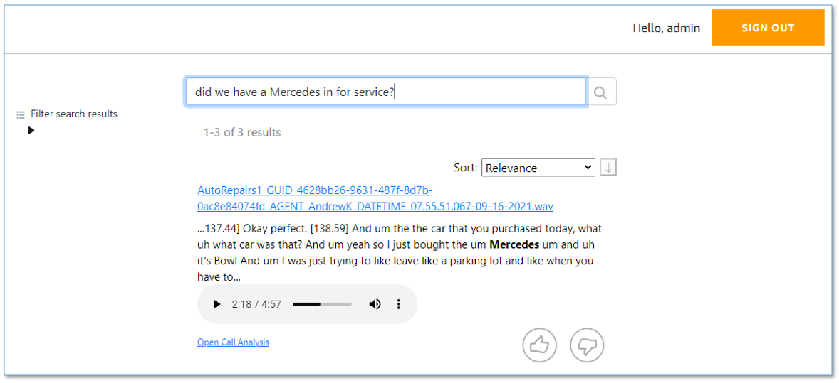
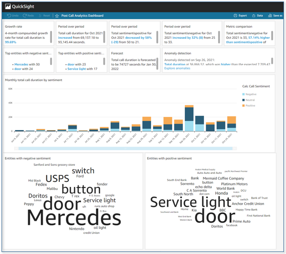
Our companion solution, Post Call Analytics (PCA), offers additional insights and analytics capabilities by using the Amazon Transcribe Call Analytics batch API to detect common issues, interruptions, silences, speaker loudness, call categories, and more. Unlike LCA, which transcribes and analyzes streaming audio in real time, PCA transcribes and analyzes your call recordings after the call has ended. Configure LCA to store call recordings to the PCA’s ingestion S3 bucket, and use the two solutions together to get the best of both worlds. For more information, see Post call analytics for your contact center with Amazon language AI services.
Conclusion
The Live Call Analytics (LCA) sample solution offers a scalable, cost-effective approach to provide live call analysis with features to assist supervisors and agents to improve focus on your callers’ experience. It uses Amazon ML services like Amazon Transcribe and Amazon Comprehend to transcribe and extract real-time insights from your contact center audio.
The sample LCA application is provided as open source—use it as a starting point for your own solution, and help us make it better by contributing back fixes and features via GitHub pull requests. For expert assistance, AWS Professional Services and other AWS Partners are here to help.
We’d love to hear from you. Let us know what you think in the comments section, or use the issues forum in the LCA GitHub repository.
About the Authors
 Bob Strahan is a Principal Solutions Architect in the AWS Language AI Services team.
 Oliver Atoa is a Principal Solutions Architect in the AWS Language AI Services team.
 Sagar Khasnis is a Senior Solutions Architect focused on building applications for Productivity Applications. He is passionate about building innovative solutions using AWS services to help customers achieve their business objectives. In his free time, you can find him reading biographies, hiking, working out at a fitness studio, and geeking out on his personal rig at home.
 Court Schuett is a Chime Specialist SA with a background in telephony and now likes to build things that build things.