The Howard and Eleanor Morgan Professor is awarded to a Cornell faculty member who has made meaningful contributions to operations research.Read More
Build a traceable, custom, multi-format document parsing pipeline with Amazon Textract
Organizational forms serve as a primary business tool across industries—from financial services, to healthcare, and more. Consider, for example, tax filing forms in the tax management industry, where new forms come out each year with largely the same information. AWS customers across sectors need to process and store information in forms as part of their daily business practice. These forms often serve as a primary means for information to flow into an organization where technological means of data capture are impractical.
In addition to using forms to capture information, over the years of offering Amazon Textract, we have observed that AWS customers frequently version their organizational forms based on structural changes made, fields added or changed, or other considerations such as a change of year or version of the form.
When the structure or content of a form changes, frequently this can cause challenges for traditional OCR systems or impact downstream tools used to capture information, even when you need to capture the same information year over year and aggregate the data for use regardless of the format of the document.
To solve this problem, in this post we demonstrate how you can build and deploy an event-driven, serverless, multi-format document parsing pipeline with Amazon Textract.
Solution overview
The following diagram illustrates our solution architecture:
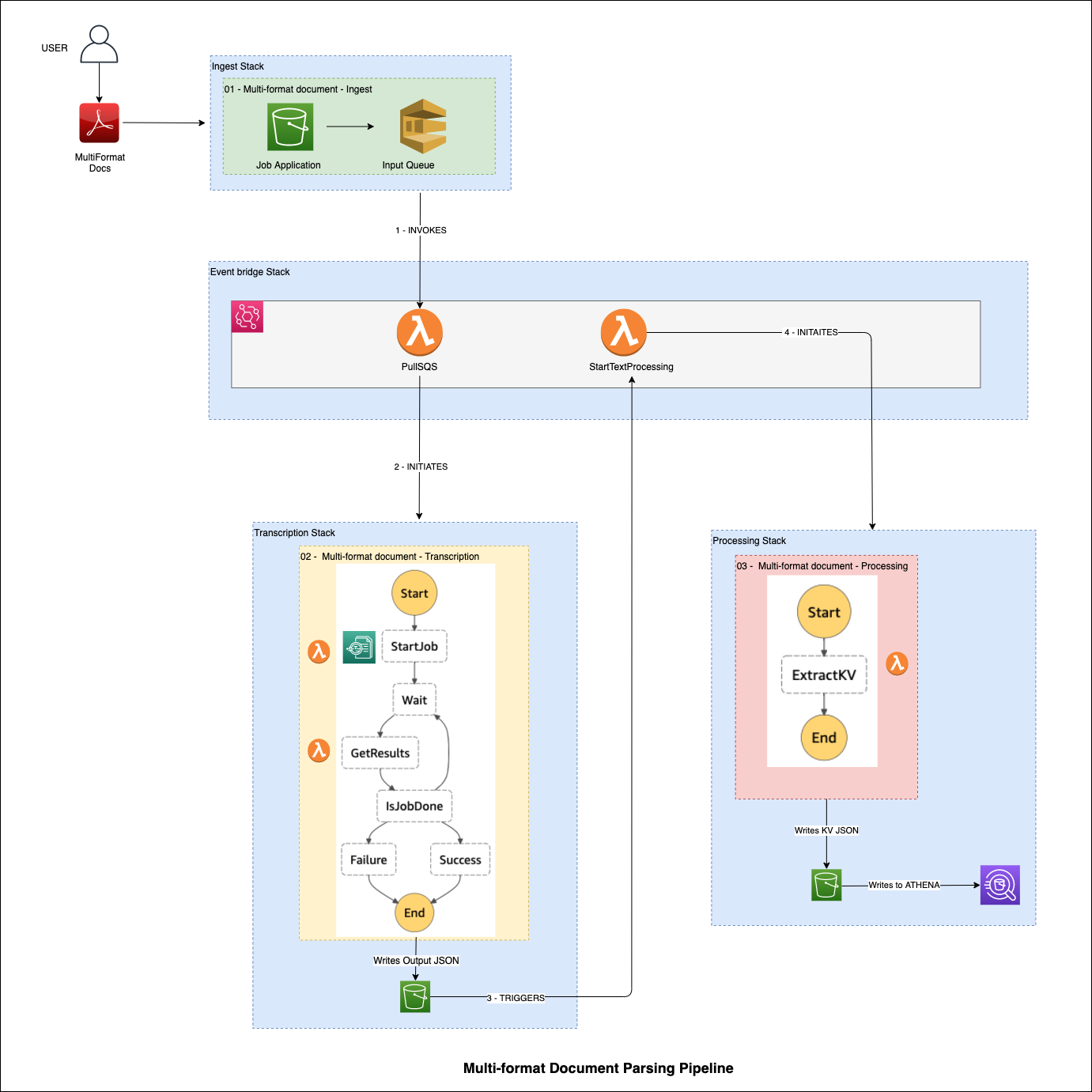
First, the solution offers pipeline ingest using Amazon Simple Storage Service (Amazon S3), Amazon S3 Event Notifications, and an Amazon Simple Queue Service (Amazon SQS) queue so that processing begins when a form lands in the target Amazon S3 partition. An event on Amazon EventBridge is created and sent to an AWS Lambda target that triggers an Amazon Textract job.
You can use serverless AWS services such as Lambda and AWS Step Functions to create asynchronous service integrations between AWS AI services and AWS Analytics and Database services for warehousing, analytics, and AI and machine learning (ML). In this post, we demonstrate how to use Step Functions to asynchronously control and maintain the state of requests to Amazon Textract asynchronous APIs. This is achieved by using a state machine for managing calls and responses. We use Lambda within the state machine to merge the paginated API response data from Amazon Textract into a single JSON object containing semi-structured text data extracted using OCR.
Then we filter across different forms using a standardized approach to aggregate this OCR data into a common structured format using Amazon Athena and a SQL Amazon Textract JSON SerDe.
You can trace the steps taken through this pipeline using serverless Step Functions to track the processing state and retain the output of each state. This is something that customers in some industries prefer to do when working with data where you must retain the results of all predictions from services such as Amazon Textract for promoting explainability of your pipeline results in the long term.
Finally, you can query the extracted data in Athena tables.
In the following sections, we walk you through setting up the pipeline using AWS CloudFormation, testing the pipeline, and adding new form versions. This pipeline provides a maintainable solution because every component (ingest, text extraction, text processing) is independent and isolated.
Define default input parameters for CloudFormation stacks
To define the input parameters for the CloudFormation stacks, open default.properties under the params folder and enter the following code:
Deploy the solution
To deploy your pipeline, complete the following steps:
- Choose Launch Stack:

- Choose Next.
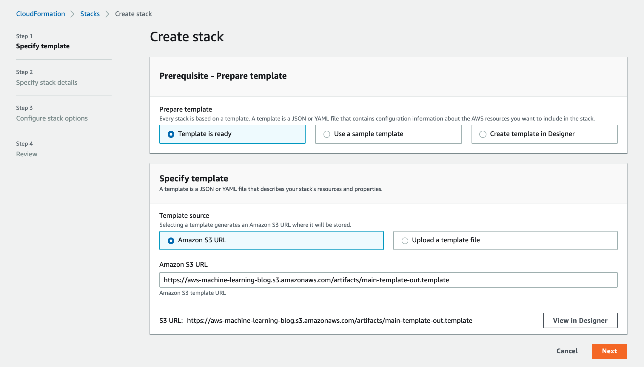
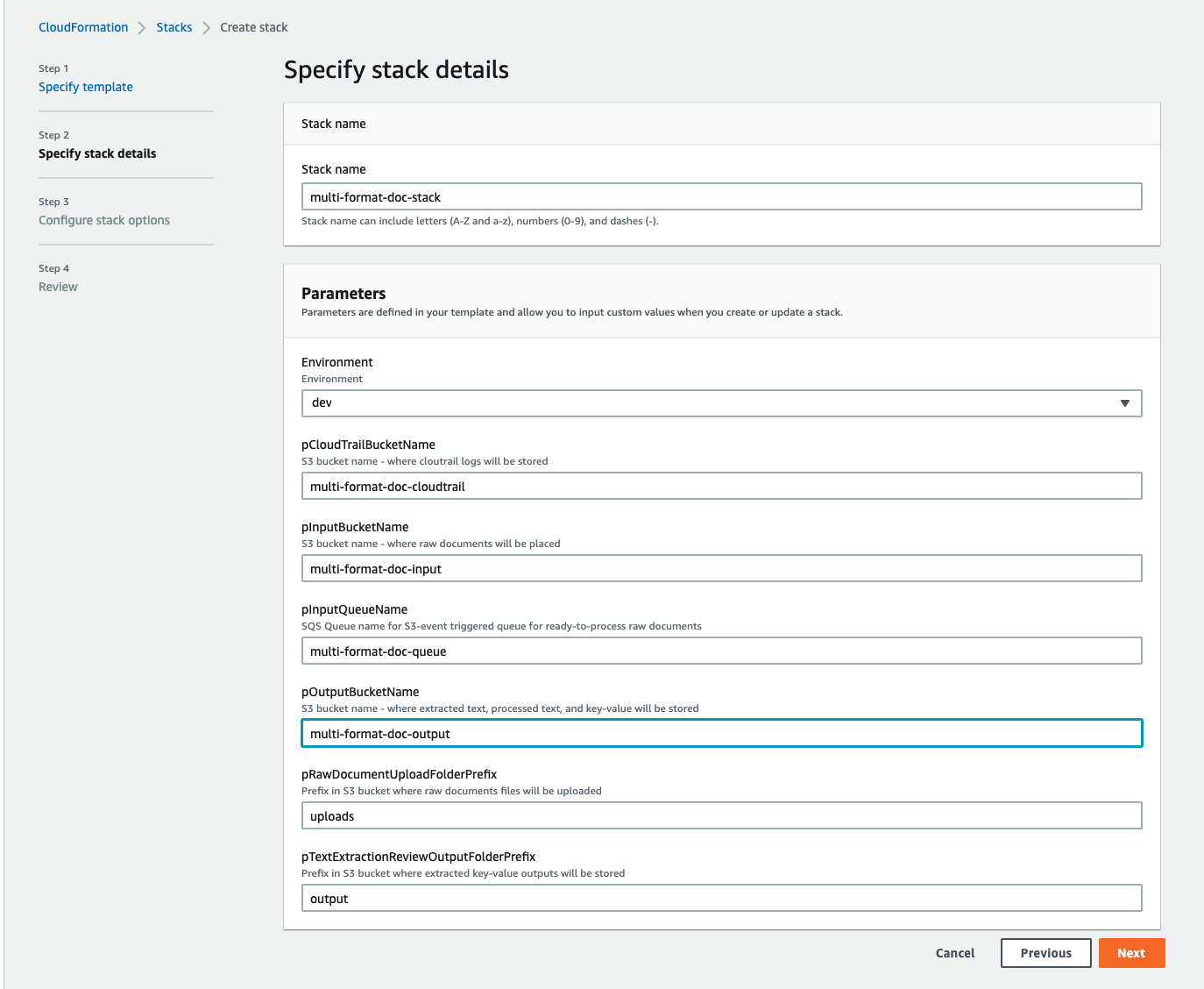
- Specify the stack details as shown in the following screenshot and choose Next.
- In the Configure stack options section, add optional tags, permissions, and other advanced settings.
- Choose Next.

- Review the stack details and select I acknowledge that AWS CloudFormation might create IAM resources with custom names.
- Choose Create stack.

This initiates stack deployment in your AWS account.

After the stack is deployed successfully, then you can start testing the pipeline as described in the next section.

Test the pipeline
After a successful deployment, complete the following steps to test your pipeline:
- Download the sample files onto your computer.
- Create an
/uploadsfolder (partition) under the newly created input S3 bucket.
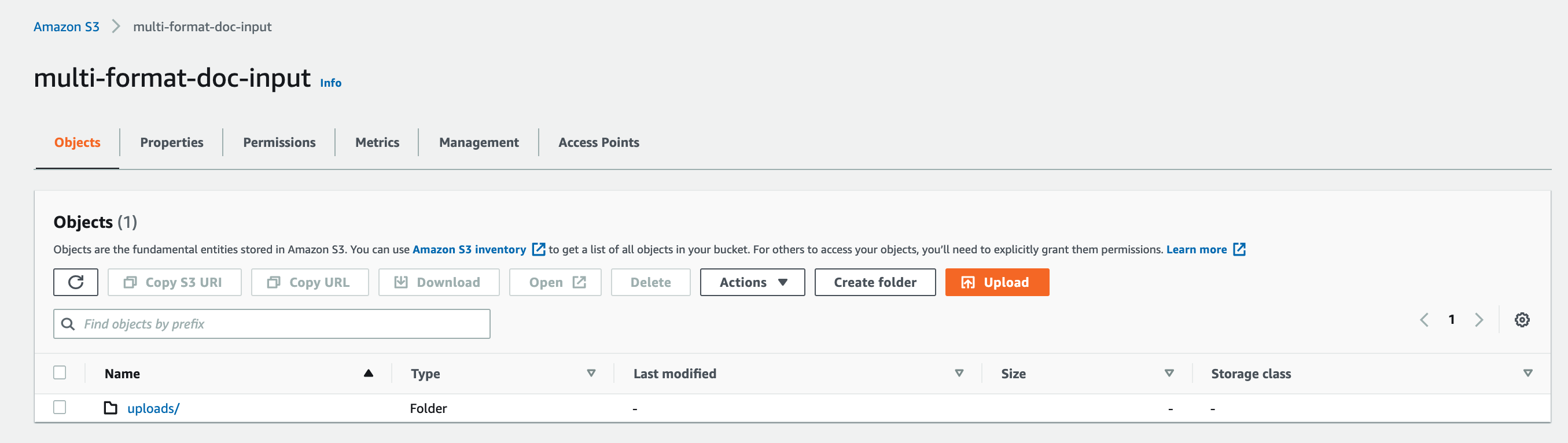
- Create the separate folders (partitions) like
jobapplicationsunder/uploads.

- Upload the first version of the job application from the sample docs folder to the
/uploads/jobapplicationspartition.

When the pipeline is complete, you can find the extracted key-value for this version of the document in /OuputS3/03-textract-parsed-output/jobapplications on the Amazon S3 console.

You can also find it in the Athena table (applications_data_table) on the Database menu (jobapplicationsdatabase).

- Upload the second version of the job application from the sample docs folder to the
/uploads/jobapplicationspartition.

When the pipeline is complete, you can find the extracted key-value for this version in /OuputS3/03-textract-parsed-output/jobapplications on the Amazon S3 console.

You can also find it in the Athena table (applications_data_table) on the Database menu (jobapplicationsdatabase).

You’re done! You’ve successfully deployed your pipeline.
Add new form versions
Updating the solution for a new form version is straightforward—each form version only needs to be updated by testing the queries in the processing stack.
After you make the updates, you can redeploy the updated pipeline using AWS CloudFormation APIs and process new documents, arriving at the same standard data points for your schema with minimal disruption and development effort needed to make changes to your pipeline. This flexibility, which is achieved by decoupling the parsing and extraction behavior and using the JSON SerDe functionality in Athena, makes this pipeline a maintainable solution for any number of form versions that your organization needs to process to gather information.
As you run the ingest solution, data from incoming forms is automatically populated to Athena with information about the files and inputs associated to them. When the data in your forms moves from unstructured to structured data, it’s ready to use for downstream applications such as analytics, ML modeling, and more.
Clean up
To avoid incurring ongoing charges, delete the resources you created as part of this solution when you’re done.
- On the Amazon S3 console, manually delete the buckets you created as part of the CloudFormation stack.
- On the AWS CloudFormation console, choose Stacks in the navigation pane.
- Select the main stack and choose Delete.
This automatically deletes the nested stacks.

Conclusion
In this post, we demonstrated how customers seeking to trace and customize the document processing can build and deploy an event-driven, serverless, multi-format document parsing pipeline with Amazon Textract. This pipeline provides a maintainable solution because every component (ingest, text extraction, text processing) are independent and isolated, allowing organizations to operationalize their solutions to address diverse processing needs.
Try the solution today and leave your feedback in the comments section.
About the Authors
 Emily Soward is a Data Scientist with AWS Professional Services. She holds a Master of Science with Distinction in Artificial Intelligence from the University of Edinburgh in Scotland, United Kingdom with emphasis on Natural Language Processing (NLP). Emily has served in applied scientific and engineering roles focused on AI-enabled product research and development, operational excellence, and governance for AI workloads running at organizations in the public and private sector. She contributes to customer guidance as an AWS Senior Speaker and recently, as an author for AWS Well-Architected in the Machine Learning Lens.
 Sandeep Singh is a Data Scientist with AWS Professional Services. He holds a Master of Science in Information Systems with concentration in AI and Data Science from San Diego State University (SDSU), California. He is a full stack Data Scientist with a strong computer science background and Trusted adviser with specialization in AI Systems and Control design. He is passionate about helping customers to get their high impact projects in the right direction, advising and guiding them in their Cloud journey, and building state-of-the-art AI/ML enabled solutions.
Nadia Carlsten drives Amazon’s quest for a quantum breakthrough
The senior product manager leading hardware and software product development at the Center for Quantum Computing wants to make fault-tolerant quantum computing a reality.Read More
Amazon SageMaker JumpStart models and algorithms now available via API
In December 2020, AWS announced the general availability of Amazon SageMaker JumpStart, a capability of Amazon SageMaker that helps you quickly and easily get started with machine learning (ML). JumpStart provides one-click fine-tuning and deployment of a wide variety of pre-trained models across popular ML tasks, as well as a selection of end-to-end solutions that solve common business problems. These features remove the heavy lifting from each step of the ML process, making it easier to develop high-quality models and reducing time to deployment.
Previously, all JumpStart content was available only through Amazon SageMaker Studio, which provides a user-friendly graphical interface to interact with the feature. Today, we’re excited to announce the launch of easy-to-use JumpStart APIs as an extension of the SageMaker Python SDK. These APIs allow you to programmatically deploy and fine-tune a vast selection of JumpStart-supported pre-trained models on your own datasets. This launch unlocks the usage of JumpStart capabilities in your code workflows, MLOps pipelines, and anywhere else you’re interacting with SageMaker via SDK.
In this post, we provide an update on the current state of JumpStart’s capabilities and guide you through the usage flow of the JumpStart API with an example use case.
JumpStart overview
JumpStart is a multi-faceted product that includes different capabilities to help get you quickly started with ML on SageMaker. At the time of writing, JumpStart enables you to do the following:
- Deploy pre-trained models for common ML tasks – JumpStart enables you to solve common ML tasks with no development effort by providing easy deployment of models pre-trained on publicly available large datasets. The ML research community has put a large amount of effort into making a majority of recently developed models publicly available for use. JumpStart hosts a collection of over 300 models, spanning the 15 most popular ML tasks such as object detection, text classification, and text generation, making it easy for beginners to use them. These models are drawn from popular model hubs, such as TensorFlow, PyTorch, Hugging Face, and MXNet Hub.
- Fine-tune pre-trained models – JumpStart allows you to fine-tune pre-trained models with no need to write your own training algorithm. In ML, the ability to transfer the knowledge learned in one domain to another domain is called transfer learning. You can use transfer learning to produce accurate models on your smaller datasets, with much lower training costs than the ones involved in training the original model from scratch. JumpStart also includes popular training algorithms based on LightGBM, CatBoost, XGBoost, and Scikit-learn that you can train from scratch for tabular data regression and classification.
- Use pre-built solutions – JumpStart provides a set of 17 pre-built solutions for common ML use cases, such as demand forecasting and industrial and financial applications, which you can deploy with just a few clicks. The solutions are end-to-end ML applications that string together various AWS services to solve a particular business use case. They use AWS CloudFormation templates and reference architectures for quick deployment, which means they are fully customizable.
- Use notebook examples for SageMaker algorithms – SageMaker provides a suite of built-in algorithms to help data scientists and ML practitioners get started with training and deploying ML models quickly. JumpStart provides sample notebooks that you can use to quickly use these algorithms.
- Take advantage of training videos and blogs – JumpStart also provides numerous blog posts and videos that teach you how to use different functionalities within SageMaker.
JumpStart accepts custom VPC settings and KMS encryption keys, so that you can use the available models and solutions securely within your enterprise environment. You can pass your security settings to JumpStart within SageMaker Studio or through the SageMaker Python SDK.
JumpStart-supported ML tasks and API example Notebooks
JumpStart currently supports 15 of the most popular ML tasks; 13 of them are vision and NLP-based tasks, of which 8 support no-code fine-tuning. It also supports four popular algorithms for tabular data modeling. The tasks and links to their sample notebooks are summarized in the following table.
Depending on the task, the sample notebooks linked in the preceding table can guide you on all or a subset of the following processes:
- Select a JumpStart supported pre-trained model for your specific task.
- Host a pre-trained model, get predictions from it in real-time, and adequately display the results.
- Fine-tune a pre-trained model with your own selection of hyperparameters and deploy it for inference.
Fine-tune and deploy an object detection model with JumpStart APIs
In the following sections, we provide a step-by-step walkthrough of how to use the new JumpStart APIs on the representative task of object detection. We show how to use a pre-trained object detection model to identify objects from a predefined set of classes in an image with bounding boxes. Finally, we show how to fine-tune a pre-trained model on your own dataset to detect objects in images that are specific to your business needs, simply by bringing your own data. We provide an accompanying notebook for this walkthrough.
We walk through the following high-level steps:
- Run inference on the pre-trained model.
- Retrieve JumpStart artifacts and deploy an endpoint.
- Query the endpoint, parse the response, and display model predictions.
- Fine-tune the pre-trained model on your own dataset.
- Retrieve training artifacts.
- Run training.
Run inference on the pre-trained model
In this section, we choose an appropriate pre-trained model in JumpStart, deploy this model to a SageMaker endpoint, and show how to run inference on the deployed endpoint. All the steps are available in the accompanying Jupyter notebook.
Retrieve JumpStart artifacts and deploy an endpoint
SageMaker is a platform based on Docker containers. JumpStart uses the available framework-specific SageMaker Deep Learning Containers (DLCs). We fetch any additional packages, as well as scripts to handle training and inference for the selected task. Finally, the pre-trained model artifacts are separately fetched with model_uris, which provides flexibility to the platform. You can use any number of models pre-trained for the same task with a single training or inference script. See the following code:
Next, we feed the resources into a SageMaker Model instance and deploy an endpoint:
Endpoint deployment may take a few minutes to complete.
Query the endpoint, parse the response, and display predictions
To get inferences from a deployed model, an input image needs to be supplied in binary format along with an accept type. In JumpStart, you can define the number of bounding boxes returned. In the following code snippet, we predict ten bounding boxes per image by appending ;n_predictions=10 to Accept. To predict xx boxes, you can change it to ;n_predictions=xx , or get all the predicted boxes by omitting ;n_predictions=xx entirely.
The following code snippet gives you a glimpse of what object detection looks like. The probability predicted for each object class is visualized, along with its bounding box. We use the parse_response and display_predictions helper functions, which are defined in the accompanying notebook.
The following screenshot shows the output of an image with prediction labels and bounding boxes.

Fine-tune a pre-trained model on your own dataset
Existing object detection models in JumpStart are pre-trained either on the COCO or the VOC datasets. However, if you need to identify object classes that don’t exist in the original pre-training dataset, you have to fine-tune the model on a new dataset that includes these new object types. For example, if you need to identify kitchen utensils and run inference on a deployed pre-trained SSD model, the model doesn’t recognize any characteristics of the new image types and therefore the output is incorrect.
In this section, we demonstrate how easy it is to fine-tune a pre-trained model to detect new object classes using JumpStart APIs. The full code example with more details is available in the accompanying notebook.
Retrieve training artifacts
Training artifacts are similar to the inference artifacts discussed in the preceding section. Training requires a base Docker container, namely the MXNet container in the following example code. Any additional packages required for training are included with the training scripts in train_sourcer_uri. The pre-trained model and its parameters are packaged separately.
Run training
To run training, we simply feed the required artifacts along with some additional parameters to a SageMaker Estimator and call the .fit function:
While the algorithm trains, you can monitor its progress either in the SageMaker notebook where you’re running the code itself, or on Amazon CloudWatch. When training is complete, the fine-tuned model artifacts are uploaded to the Amazon Simple Storage Service (Amazon S3) output location specified in the training configuration. You can now deploy the model in the same manner as the pre-trained model. You can follow the rest of the process in the accompanying notebook.
Conclusion
In this post, we described the value of the newly released JumpStart APIs and how to use them. We provided links to 17 example notebooks for the different ML tasks supported in JumpStart, and walked you through the object detection notebook.
We look forward to hearing from you as you experiment with JumpStart.
About the Authors
 Dr. Vivek Madan is an Applied Scientist with the Amazon SageMaker JumpStart team. He got his PhD from University of Illinois at Urbana-Champaign and was a Post-Doctoral Researcher at Georgia Tech. He is an active researcher in machine learning and algorithm design, and has published papers in EMNLP, ICLR, COLT, FOCS, and SODA conferences.
 João Moura is an AI/ML Specialist Solutions Architect at Amazon Web Services. He is mostly focused on NLP use-cases and helping customers optimize Deep Learning model training and deployment.
 Dr. Ashish Khetan is a Senior Applied Scientist with Amazon SageMaker JumpStart and Amazon SageMaker built-in algorithms and helps develop machine learning algorithms. He is an active researcher in machine learning and statistical inference and has published many papers in NeurIPS, ICML, ICLR, JMLR, and ACL conferences.
The science behind Hunches: Deep device embeddings
A machine learning model learns representations that cluster devices according to their usage patterns.Read More
Unravel the knowledge in Slack workspaces with intelligent search using the Amazon Kendra Slack connector
Organizations use messaging platforms like Slack to bring the right people together to securely communicate with each other and collaborate to get work done. A Slack workspace captures invaluable organizational knowledge in the form of the information that flows through it as the users collaborate. However, making this knowledge easily and securely available to users is challenging due to the fragmented structure of Slack workspaces. Additionally, the conversational nature of Slack communication renders a traditional keyword-based approach to search ineffective.
You can now use the Amazon Kendra Slack connector to index Slack messages and documents, and search this content using intelligent search in Amazon Kendra, powered by machine learning (ML).
This post shows how to configure the Amazon Kendra Slack connector and take advantage of the service’s intelligent search capabilities. We use an example of an illustrative Slack workspace used by members to discuss technical topics related to AWS.
Solution overview
Slack workspaces include public channels where any workspace user can participate, and private channels where only those users who are members of these channels can communicate with each other. Furthermore, individuals can directly communicate with one another in one-on-one and ad hoc groups. This communication is in the form of messages and threads of replies, with optional document attachments. Slack workspaces of active organizations are dynamic, with its content and collaboration evolving continuously.
In our solution, we configure a Slack workspace as a data source to an Amazon Kendra search index using the Amazon Kendra Slack connector. Based on the configuration, when the data source is synchronized, the connector either crawls and indexes all the content from the workspace that was created on or before a specific date, or can optionally be based on a look back parameter in a change log mode. The look back parameter lets you crawl the date back a number of days since the last time you synced your data source. The connector also collects and ingests Access Control List (ACL) information for each indexed message and document. When access control or user context filtering is enabled, the search results of a query made by a user includes results only from those documents that the user is authorized to read.
Prerequisites
To try out the Amazon Kendra connector for Slack using this post as a reference, you need the following:
- An AWS account with privileges to create AWS Identity and Access Management (IAM) roles and policies. For more information, see Overview of access management: Permissions and policies.
- Basic knowledge of AWS and working knowledge of Slack workspace administration.
- Admin access to a Slack workspace.
Configure your Slack workspace
The following screenshot shows our example Slack workspace:

The workspace has five users as members: Workspace Admin, Generic User, DB Solutions Architect, ML Solutions Architect, and Solutions Architect. There are three public channels, #general, #random, and #test-slack-workspace, which any member can access. Regarding the secure channels, #databases has Workspace Admin and DB Solutions Architect as members, #machine-learning has Workspace Admin and ML Solutions Architect as members, and #security and #well-architected secure channels have Solutions Architect, DB Solutions Architect, ML Solutions Architect, and Workspace Admin as members. The connector-test app is configured in the Slack workspace in order to create a user OAuth token to be used in configuring the Amazon Kendra connector for Slack.
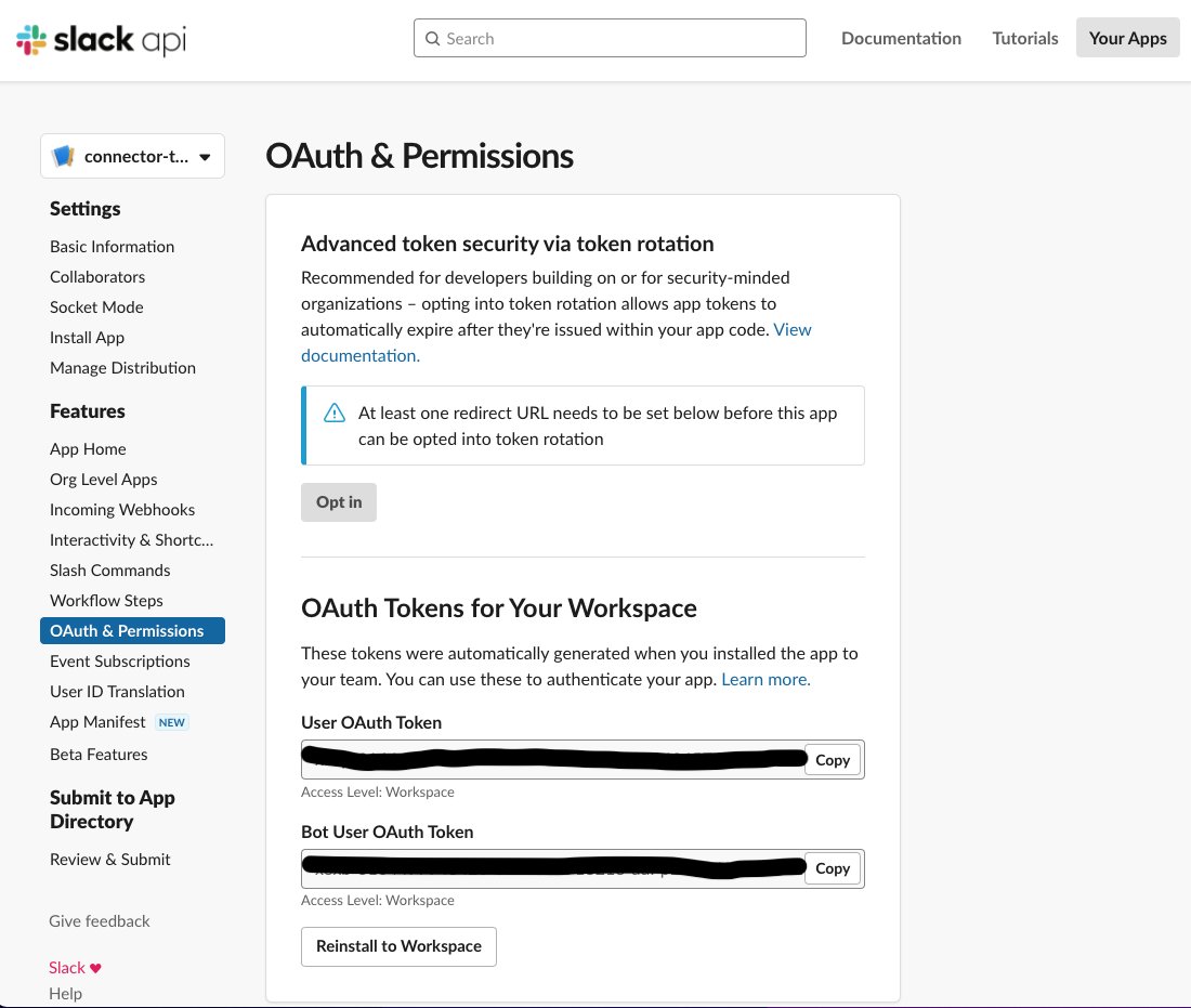
The following screenshot shows the configuration details of the connector-test app OAuth tokens for the Slack workspace. We use the user OAuth token in configuring the Amazon Kendra connector for Slack.
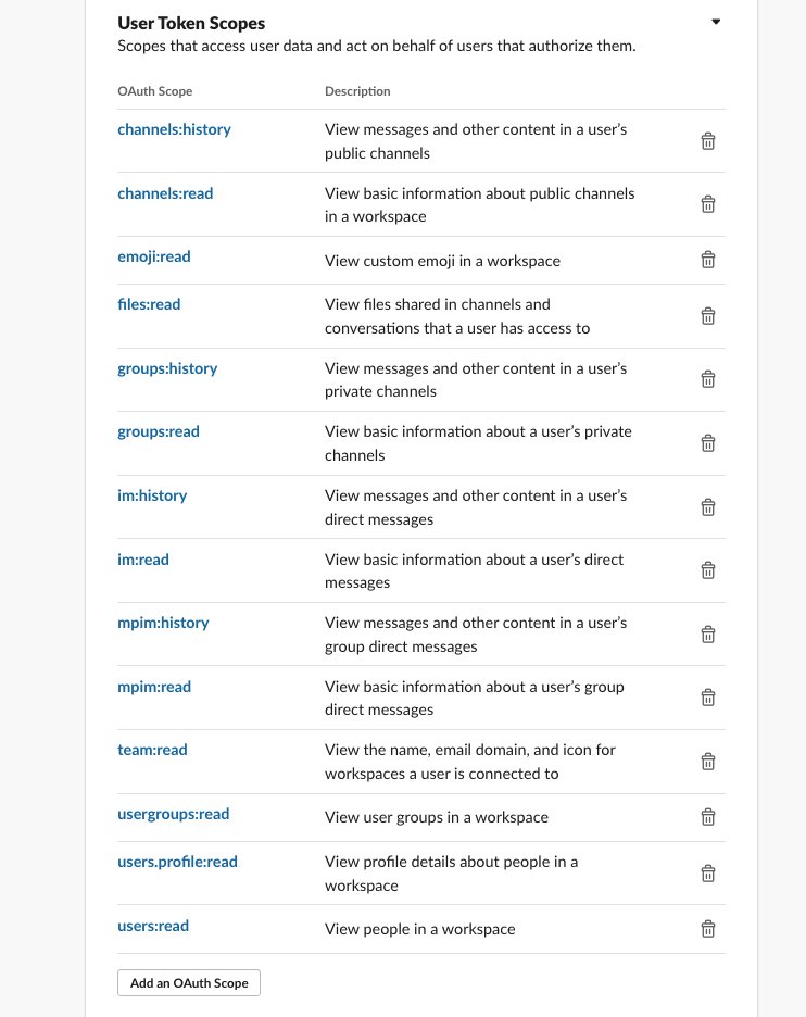
In the User Token Scopes section, we configure the connector-test app for the Slack workspace.
Configure the data source using the Amazon Kendra connector for Slack
To add a data source to your Amazon Kendra index using the Slack connector, you can use an existing Amazon Kendra index, or create a new Amazon Kendra index. Then complete the steps below. For more information on this topic, please refer to the section on Amazon Kendra connector for Slack in the Amazon Kendra Developer Guide.
- On the Amazon Kendra console, open the index and choose Data sources in the navigation pane.
- Under Slack, choose Add data source.
- Choose Add connector.

- In the Specify data source details section, enter the details of your data source and choose Next.
- In the Define access and security section, for Slack workspace team ID, enter the ID for your workspace.
- Under Authentication, you can either choose Create to add a new secret using the user OAuth token created for the
connector-app, or use an existing AWS Secrets Manager secret that has the user OAuth token for the workspace that you want the connector to access. - For IAM role, you can choose Create a new role or choose an existing IAM role configured with appropriate IAM policies to access the Secrets Manager secret, Amazon Kendra index, and data source.
- Choose Next.

- In the Configure sync settings section, provide information regarding your sync scope and run schedule.
- Choose Next.

- In the Set field mappings section, you can optionally configure the field mappings, or how the Slack field names are mapped to Amazon Kendra attributes or facets.
- Choose Next.
- Review your settings and confirm to add the data source.
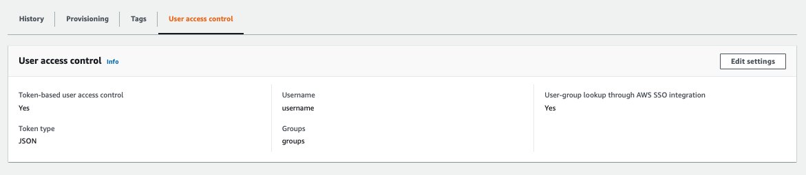
When the data source sync is complete, the User access control tab for the Amazon Kendra index is enabled. Note that in order to use the ACLs for Slack connector, it’s not necessary to enable User-group lookup through AWS SSO integration, though it is enabled in the following screenshot.
While making search queries, we want to interact with facets such as the channels of the workspace, category of the document, and the authors.
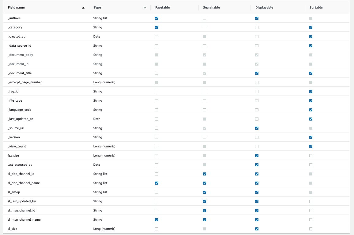
- Choose Facet definition in the navigation pane.
- Select the checkbox in the Facetable column for the facets
_authors,_category,sl_doc_channel_name, andsl_msg_channel_name.
Search with Amazon Kendra
Now we’re ready to make a few queries on the Amazon Kendra search console by choosing Search indexed content in the navigation pane.
In the first query, the user name is set to the email address of Generic User. The following screenshot shows the query response. Note that we get an answer from the aws-overview.pdf document posted in #general channel, followed by a few results from relevant documents or messages. The facets show the categories of the results to be MESSAGE and FILE. The sl_doc_channel_name facet includes the information that the document is from #general channel, the sl_msg_channel_name includes the information that there are results from all the open channels (namely #random, #general, and #test-slack-workspace), and the authors facet includes the names of the authors of the messages.

Now let’s set the user name to be the email address corresponding to the user Solutions Architect. The following screenshot shows the query response. In addition to the public channels, the results also include secure channels #security and #well-architected.
In the next query, we set the user name to be the email address of the ML Solutions Architect. In this case, the results contain the category of THREAD_REPLY in addition to MESSAGE and FILE. Also, ML Solutions Architect can access the secure channel of #machine-learning.

Now for the same query, to review what people have replied to the question, select the THREAD_REPLY category on the left to refine the results. The response now contains only those results that are of the THREAD_REPLY category.

The results from the response include the URL to the Slack message. When you choose the suggested answer result in the response, the URL asks for Slack workspace credentials, and opens the thread reply being referenced.

Clean up
To avoid incurring future costs, clean up the resources you created as part of this solution. If you created a new Amazon Kendra index while testing this solution, delete it. If you only added a new data source using the Amazon Kendra connector for Slack, delete that data source.
Conclusion
Using the Amazon Kendra Slack connector organizations can make invaluable information trapped in their Slack workspaces available to their users securely using intelligent search powered by Amazon Kendra. Additionally, the connector provides facets for Slack workspace attributes such as channels, authors, and categories for the users to interactively refine the search results based on what they’re looking for.
To learn more about the Amazon Kendra connector for Slack, please refer to the section on Amazon Kendra connector for Slack in the Amazon Kendra Developer Guide.
For more information on how you can create, modify, or delete metadata and content when ingesting your data from the Slack workspace, refer to Customizing document metadata during the ingestion process and Enrich your content and metadata to enhance your search experience with custom document enrichment in Amazon Kendra.
About the Author
 Abhinav Jawadekar is a Senior Partner Solutions Architect at Amazon Web Services. Abhinav works with AWS Partners to help them in their cloud journey.
Securely search unstructured data on Windows file systems with the Amazon Kendra connector for Amazon FSx for Windows File Server
Critical information can be scattered across multiple data sources in your organization, including sources such as Windows file systems stored on Amazon FSx for Windows File Server. You can now use the Amazon Kendra connector for FSx for Windows File Server to index documents (HTML, PDF, MS Word, MS PowerPoint, and plain text) stored in your Windows file system on FSx for Windows File Server and search for information across this content using intelligent search in Amazon Kendra.
Organizations store unstructured data in files on shared Windows file systems and secure it by using Windows Access Control Lists (ACLs) to ensure that users can read, write, and create files as per their access permissions configured in the enterprise Active Directory (AD) domain. Finding specific information from this data not only requires searching through the files, but also ensuring that the user is authorized to access it. The Amazon Kendra connector for FSx for Windows File Server indexes the files stored on FSx for Windows File Server and ingests the ACLs in the Amazon Kendra index, so that the response of a search query made by a user includes results only from those documents that the user is authorized to read.
This post takes the example of a set of documents stored securely on a file system using ACLs on FSx for Windows File Server. These documents are ingested in an Amazon Kendra index by configuring and synchronizing this file system as a data source of the index using the connector for FSx for Windows File Server. Then we demonstrate that when a user makes a search query, the Amazon Kendra index uses the ACLs based on the user name and groups the user belongs to, and returns only those documents the user is authorized to access. We also include details of the configuration and screenshots at every stage so you can use this as a reference when configuring the Amazon Kendra connector for FSx for Windows File Server in your setup.
Prerequisites
To try out the Amazon Kendra connector for FSx for Windows File Server, you need the following:
- An AWS account with privileges to create AWS Identity and Access Management (IAM) roles and policies. For more information, see Overview of access management: Permissions and policies.
- Basic knowledge of AWS and working knowledge of Windows ACLs and Microsoft AD domain administration.
- Admin access to a file system on FSx for Windows File Server, with admin access to the AD domain to which it belongs. Alternately, you can deploy this using the Quick Start for FSx for Windows File Server.
- The AWS_Whitepapers.zip, which we use to try out the functionality. For updated versions, refer to AWS Whitepapers & Guides. Alternately, you can use your own documents.
Solution architecture
The following diagram illustrates the solution architecture:
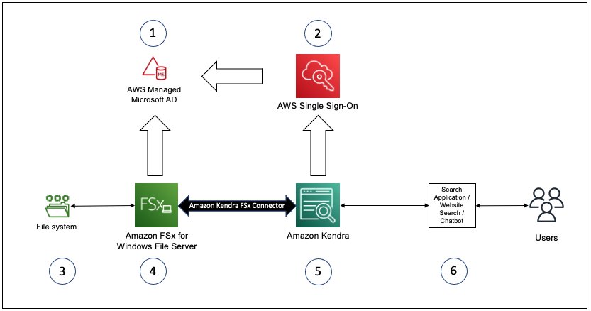
The documents in this example are stored on a file system (3 in the diagram) on FSx for Windows File Server (4). The files are set up with ACLs based on the user and group configurations in the AD domain created using AWS Directory Service (1) to which FSx for Windows File Server belongs. This file system on FSx for Windows File Server is configured as a data source for Amazon Kendra (5). AWS Single Sign On (AWS SSO) is enabled with the AD as the identity source, and the Amazon Kendra index is set up to use AWS SSO (2) for user name and group lookup for the user context of the search queries from the customer search solution deployments (6). The FSx for Windows File Server file system, AWS Managed Microsoft AD server, the Amazon Virtual Private Cloud (Amazon VPC) and subnets configured in this example are created using the Quick Start for FSx for Windows File Server.
FSx for Windows File Server configuration
The following screenshot shows the file system on FSx for Windows File Server configured as a part of an AWS Managed Microsoft AD domain that is used in our example, as seen on the Amazon FSx console.

AWS Managed Microsoft AD configuration
The AD to which FSx for Windows File Server belongs is configured as an AWS Managed Microsoft AD, as seen in the following screenshot of the Directory Service console.

Users, groups and ACL configuration for sample dataset
For this post, we used a dataset consisting of a few AWS publicly available whitepapers and stored them in directories based on their categories (Best_Practices, Databases, General, Machine_Learning, Security, and Well_Architected) on a file system on FSx for Windows File Server. The following screenshot shows the folders as seen from a Windows bastion host that is part of the AD domain to which the file system belongs.

Users and groups are configured in the AD domain as follows:
-
kadmin –
group_kadmin -
patricia –
group_sa,group_kauthenticated -
james –
group_db_sa,group_kauthenticated -
john –
group_ml_sa,group_kauthenticated -
mary, julie, tom –
group_kauthenticated
The following screenshot shows users and groups configured in the AWS Managed Microsoft AD domain as seen from the Windows bastion host.
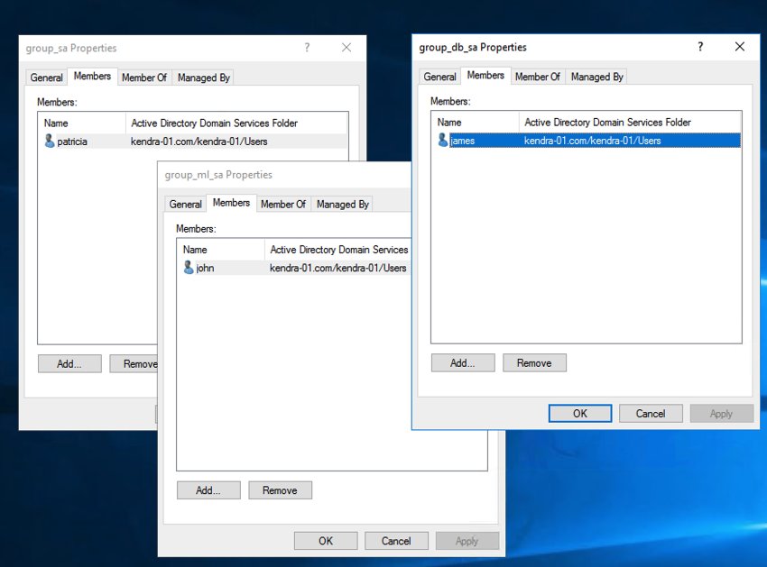
The ACLs for the files in each directory are set up based on the user and group configurations in the AD domain to which FSx for Windows File Server belongs:
-
All authenticated users (group_kauthenticated) – Can access the documents in
Best_PracticesandGeneraldirectories -
Solutions Architects (group_sa) – Can access the documents in
Best_Practices,General,Security, andWell_Architecteddirectories -
Database subject matter expert Solutions Architects (group_db_sa) – Can access the documents in
Best_Practices,General,Security,Well_Architected, andDatabasedirectories -
Machine learning subject matter expert Solutions Architects (group_ml_sa) – Can access
Best_Practices,General,Security,Well_Architected, andMachine_Learningdirectories - Admin (group_kadmin) – Can access the documents in any of the six directories
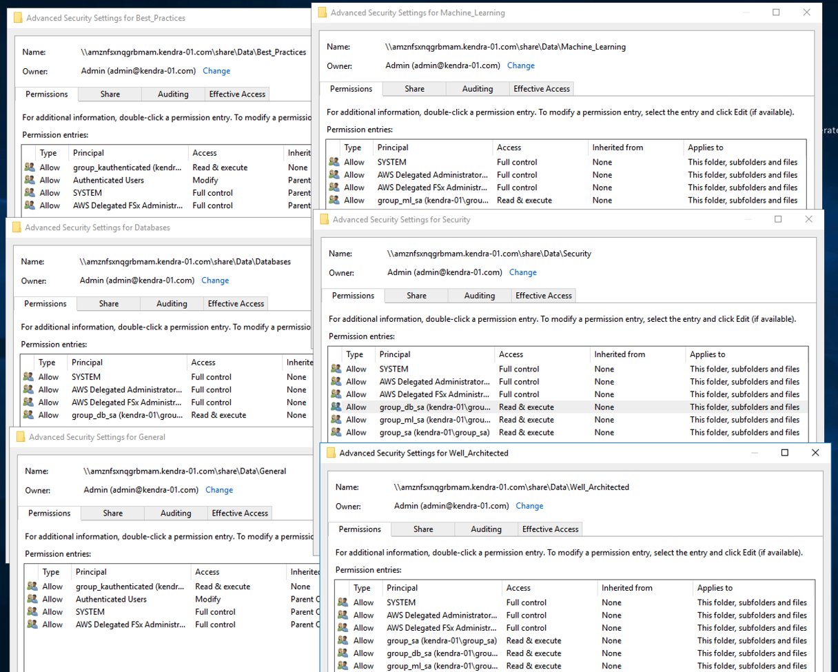
The following screenshot shows the ACL configurations for each of the directories of our sample data, as seen from the Windows bastion host.
AWS Single Sign-On configuration
AWS SSO is configured with the AD domain as the identity source. The following screenshot shows the settings on the AWS SSO console.

The groups are synchronized in AWS SSO from the AD, as shown in the following screenshot.

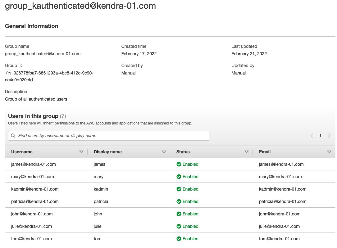
The following screenshot shows the members of the group_kauthenticated group synchronized from the AD.
Data source configuration using Amazon Kendra connector for FSx for Windows File Server
We configure a data source using the Amazon Kendra connector for FSx for Windows File Server in an Amazon Kendra index on the Amazon Kendra console. You can create a new Amazon Kendra index or use an existing one and add a new data source.
When you add a data source for an Amazon Kendra index, choose the FSx for Windows File Server connector by choosing Add connector under Amazon FSx.

The steps to add a data source name and resource tags are similar to adding any other data source, as shown in the following screenshot.

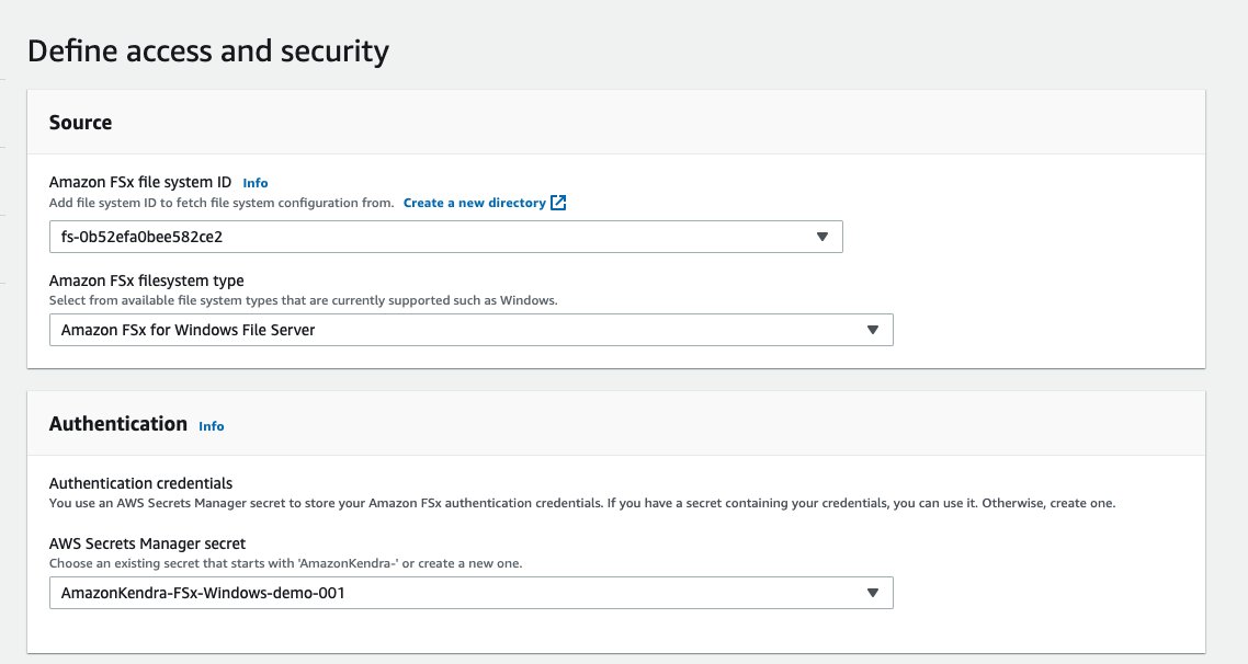
The details for configuring the specific file system on Amazon FSx and the type of the file system (FSx for Windows File Server in this case), are configured for in the Source section. The authentication credentials of a user with admin privileges to the file system are configured using an AWS Secrets Manager secret.
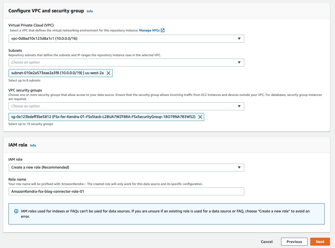
The VPC and security group settings of the data source configuration include the details of the VPC, subnets, and security group of Amazon FSx and the AD server. In the following screenshot, we also create a new IAM role for the data source.
The next step in data source configuration involves mapping the Amazon FSx connector fields to the Amazon Kendra facets or field names. In the following screenshot, we leave the configuration unchanged. The step after this involves reviewing the configuration and confirming that the data source should be created.

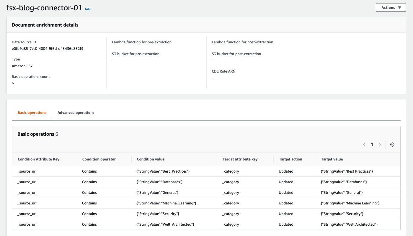
After you configure the file system on FSx for Windows File Server, where the example data is stored as a data source, you configure Custom Document Enrichment (CDE) basic operations for this data source so that the Amazon Kendra index filed _category is configured based on the directory in which a document is stored. The data source sync is started after the CDE configuration, so that the _category attributes for the documents get configured during the ingestion workflow.
As shown in the following screenshot, the Amazon Kendra index user access control settings are configured for user and group lookup through AWS SSO integration. JSON token-based user access control is enabled to search based on user and group names from the Amazon Kendra Search console.

In the facet definition for the Amazon Kendra index, make sure that the facetable and displayable boxes are checked for _category. This allows you to use the _category values set by the CDE basic operations as facets while searching.

Search with Amazon Kendra
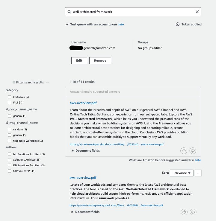
After the data source sync is complete, we can start searching from the Amazon Kendra Search console, by choosing Search indexed content in the navigation pane on the Amazon Kendra console. Because we’re using AWS whitepapers as the dataset to ingest in the Amazon Kendra index, we use “What’s DynamoDB?” as the search query. Only authenticated users are authorized access to the files on the file system on FSx for Windows File Server; therefore, when we use this search query without setting any user name or group, we don’t get any results.

Now let’s set the user name to mary@kendra-01.com. The user mary belongs to group_kauthenticated, and therefore is authorized to access the documents in the Best_Practices and General directories. In the following screenshot, the search response includes documents with the facet category set to Best Practices and General. The CDE basic operations set the facet category depending on the directory names contained in the source_uri. This confirms that the ACLs ingested in Amazon Kendra by the connector for FSx for Windows File Server are being enforced in the search results based on the user name.

Now we change the user name to patricia@kendra-01.com. The user patricia belongs to group_sa, with access to the Security and Well_Architected directories, in addition to Best_Practices and General directories. The search response includes results from these additional directories.

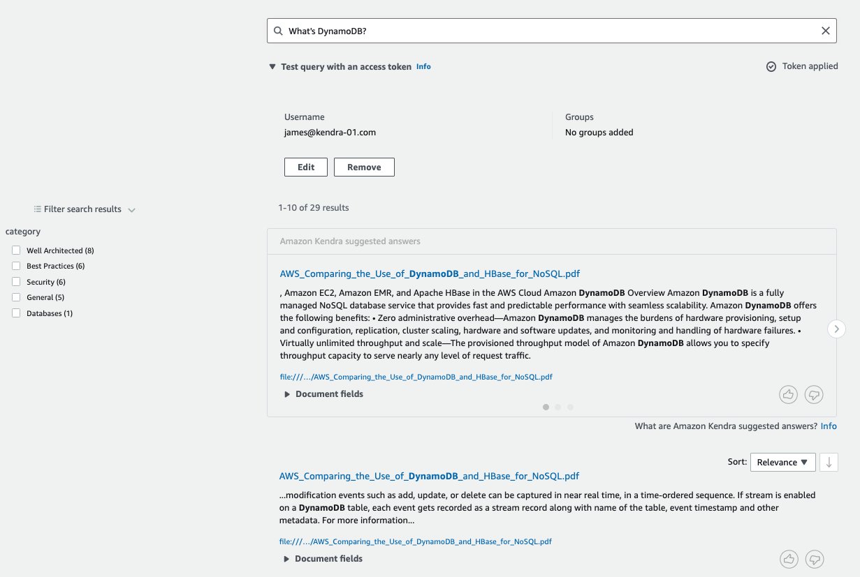
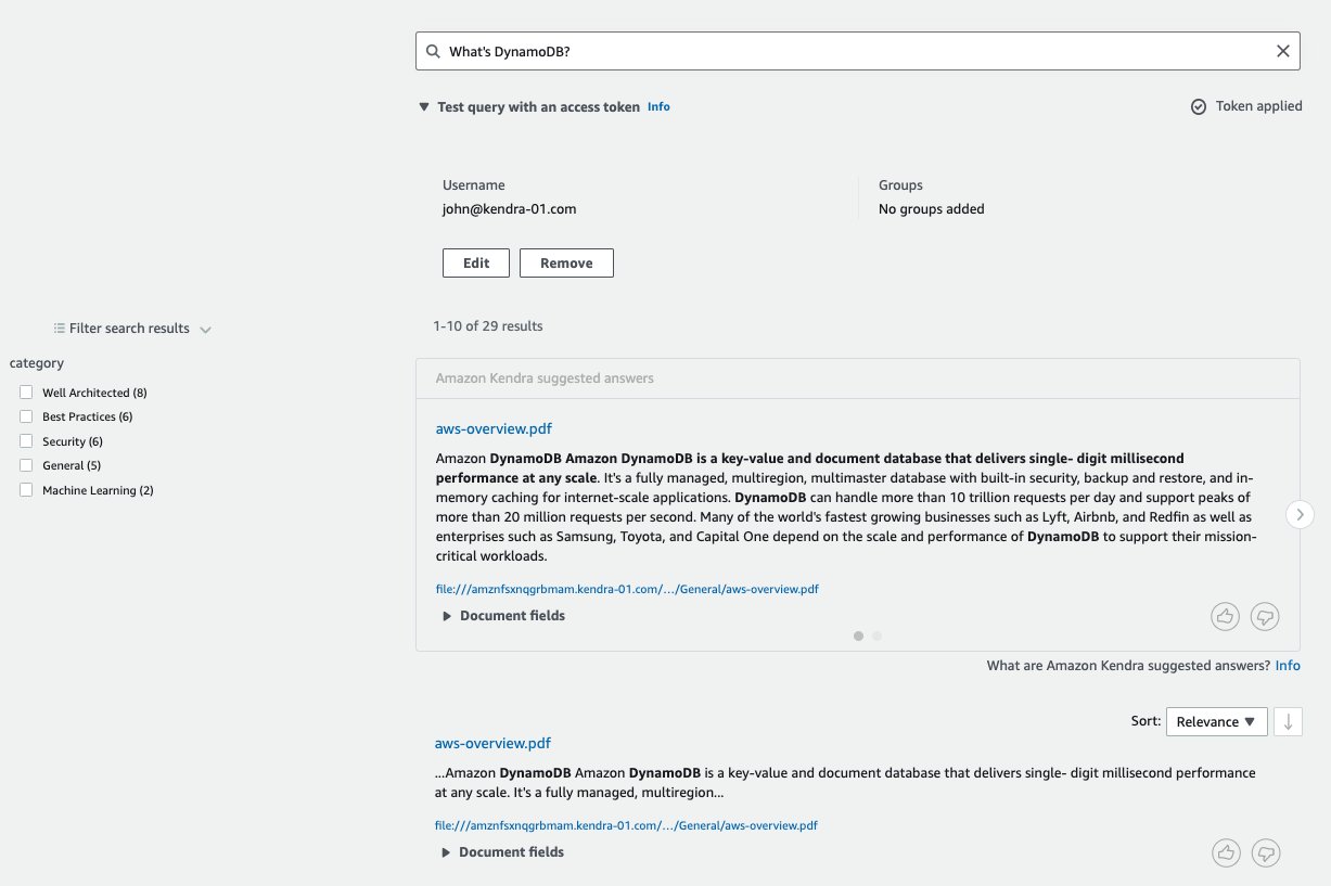
Now we can observe how the results from the search response change as we change the user name to james@kendra-01.com, john@kendra-01.com, and kadmin@kendra-01.com in the following screenshots.

Clean up
If you deployed any AWS infrastructure to experiment with the Amazon Kendra connector for FSx for Windows File Server, clean up the infrastructure as follows:
- If you used the Quick Start for FSx for Windows File Server, delete the AWS CloudFormation stack you created so that it deletes all the resources it created.
- If you created a new Amazon Kendra index, delete it.
- If you only added a new data source using the connector, delete that data source.
- Delete the AWS SSO configuration.
Conclusion
The Amazon Kendra connector for FSx for Windows File Server enables secure and intelligent search of information scattered in unstructured content. The data is securely stored on file systems on FSx Windows File Server with ACLs and shared with users based on their Microsoft AD domain credentials.
For more information on the Amazon Kendra connector for FSx for Windows File Server, refer to Getting started with an Amazon FSx data source (console) and Using an Amazon FSx data source.
For information on Custom Document Enrichment, refer to Customizing document metadata during the ingestion process and Enrich your content and metadata to enhance your search experience with custom document enrichment in Amazon Kendra.
About the Author
Abhinav Jawadekar is a Senior Partner Solutions Architect at Amazon Web Services. Abhinav works with AWS Partners to help them in their cloud journey.
Registration opens for Amazon re:MARS event
In-person event featuring some of the brightest leaders in science, academia, and business is planned for June 21-24 in Las VegasRead More
Automate email responses using Amazon Comprehend custom classification and entity detection
In this post, we demonstrate how to create an automated email response solution using Amazon Comprehend.
Organizations spend lots of resources, effort, and money on running their customer care operations to answer customer questions and provide solutions. Your customers may ask questions via various channels, such as email, chat, or phone, and deploying a workforce to answer those queries can be resource intensive, time-consuming, and even unproductive if the answers to those questions are repetitive.
During the COVID-19 pandemic, many organizations couldn’t adequately support their customers due to the shutdown of customer care and agent facilities, and customer queries were piling up. Some organizations struggled to reply to queries promptly, which can cause a poor customer experience. This in turn can result in customer dissatisfaction, and can impact an organization’s reputation and revenue in the long term.
Although your organization might have the data assets for customer queries and answers, you may still struggle to implement an automated process to reply to your customers. Challenges might include unstructured data, different languages, and a lack of expertise in artificial intelligence (AI) and machine learning (ML) technologies.
You can overcome such challenges by using Amazon Comprehend to automate email responses to customer queries. With our solution, you can identify the intent of customer emails send an automated response if the intent matches your existing knowledge base. If the intent doesn’t have a match, the email goes to the support team for a manual response. The following are some common customer intents when contacting customer care:
- Transaction status (for example, status of a money transfer)
- Password reset
- Promo code or discount
- Hours of operation
- Find an agent location
- Report fraud
- Unlock account
- Close account
Amazon Comprehend can help you perform classification and entity detection on emails for any of the intents above. For this solution, we show how to classify customer emails for the first three intents. You can also use Amazon Comprehend to detect key information from emails, so you can automate your business processes. For example you can use Amazon Comprehend to automate the reply to a customer request with specific information related to that query.
Solution overview
To build our customer email response flow, we use the following services:
- Amazon Comprehend
- AWS Lambda
- Amazon Simple Email Service (Amazon SES)
- Amazon Simple Notification Service (Amazon SNS)
- Amazon WorkMail
The following architecture diagram highlights the end-to-end solution:

The solution workflow includes the following steps:
- A customer sends an email to the customer support email created in WorkMail.
- WorkMail invokes a Lambda function upon receiving the email.
- The function sends the email content to a custom classification model endpoint.
- The custom classification endpoint returns with a classified value and confidence level (over 80%, but you can configure this as needed).
- If the classification value is
MONEYTRANSFER, the Lambda function calls the entity detection endpoint to find the money transfer ID. - If the money transfer ID is returned, the function returns the money transfer status randomly (in real-world scenario, you can call the database via API to fetch the actual transfer status).
- Based on the classified value returned, a predefined email template in Amazon SES is chosen, and a reply email is sent to the customer.
- If the confidence level is less than 80%, a classified value is not returned, or entity detection doesn’t find the money transfer ID, the customer email is pushed to an SNS topic. You can subscribe to Amazon SNS to push the message to your ticketing system.
Prerequisites
Refer to the README.md file in the GitHub repo to make sure you meet the prerequisites to deploy this solution.
Deploy the solution
Solution deployment consists of the following high-level steps:
- Complete manual configurations using the AWS Management Console.
- Run scripts in an Amazon SageMaker notebook instance using the provided notebook file.
- Deploy the solution using the AWS Cloud Development Kit (AWS CDK).
For full instructions, refer to the README.md file in the GitHub repo.
Test the solution
To test the solution, send an email from your personal email to the support email created as part of the AWS CDK deployment (for this post, we use support@mydomain.com). We use the following three intents in our sample data for custom classification training:
- MONEYTRANSFER – The customer wants to know the status of a money transfer
- PASSRESET – The customer has a login, account locked, or password request
- PROMOCODE – The customer wants to know about a discount or promo code available for a money transfer
The following screenshot shows a sample customer email:

If the customer email is not classified or confidence levels are below 80%, the content of the email is forwarded to an SNS topic. Whoever is subscribed to the topic receives the email content as a message. We subscribed to this SNS topic with the email that we passed with the human_workflow_email parameter during the deployment.
Clean up
To avoid incurring ongoing costs, delete the resources you created as part of this solution when you’re done.
Conclusion
In this post, you learned how to configure an automated email response system using Amazon Comprehend customer classification and entity detection and other AWS services. This solution can provide the following benefits:
- Improved email response time
- Improved customer satisfaction
- Cost savings regarding time and resources
- Ability to focus on key customer issues
You can also expand this solution to other areas in your business and to other industries.
With the current architecture, the emails that are classified with a low confidence score are routed to a human loop for manual verification and response. You can use the inputs from the manual review process to further improve the Amazon Comprehend model and increase the automated classification rate. Amazon Augmented AI (Amazon A2I) provides built-in human review workflows for common ML use cases, such as NLP-based entity recognition in documents. This allows you to easily review predictions from Amazon Comprehend.
As we get more data for every intent, we will retrain and deploy the custom classification model and update the email response flow accordingly in the GitHub repo.
About the Author
 Godwin Sahayaraj Vincent is an Enterprise Solutions Architect at AWS who is passionate about Machine Learning and providing guidance to customers to design, deploy and manage their AWS workloads and architectures. In his spare time, he loves to play cricket with his friends and tennis with his three kids.
 Shamika Ariyawansa is an AI/ML Specialist Solutions Architect on the Global Healthcare and Life Sciences team at Amazon Web Services. He works with customers to advance their ML journey with a combination of AWS ML offerings and his ML domain knowledge. He is based out of Denver, Colorado. In his spare time, he enjoys off-roading adventures in the Colorado mountains and competing in machine learning competitions.
Real-world robotic-manipulation system
Amazon Research Award recipient Russ Tedrake is teaching robots to manipulate a wide variety of objects in unfamiliar and constantly changing contexts.Read More