Amazon SageMaker Data Wrangler is the fastest and easiest way for data scientists to prepare data for machine learning (ML) applications. With Data Wrangler, you can simplify the process of feature engineering and complete each step of the data preparation workflow, including data selection, cleansing, exploration, and visualization through a single visual interface. Data Wrangler comes with 300 built-in data transformation recipes that you can use to quickly normalize, transform, and combine features. With the data selection tool in Data Wrangler, you can quickly select data from different data sources, such as Amazon Simple Storage Service (Amazon S3), Amazon Athena, and Amazon Redshift.

AWS Lake Formation cross-account capabilities simplify securing and managing distributed data lakes across multiple accounts through a centralized approach, providing fine-grained access control to Athena tables.

In this post, we demonstrate how to enable cross-account access for Data Wrangler using Athena as a source and Lake Formation as a central data governance capability. As shown in the following architecture diagram, Account A is the data lake account that holds all the ML-ready data derived from ETL pipelines. Account B is the data science account where a team of data scientists uses Data Wrangler to compile and run data transformations. We need to enable cross-account permissions for Data Wrangler in Account B to access the data tables located in Account A’s data lake via Lake Formation permissions.

With this architecture, data scientists and engineers outside the data lake account can access data from the lake and create data transformations via Data Wrangler.

Before you dive into the setup process, ensure the data to be shared across accounts are crawled and cataloged as detailed in this post. Let us presume this process has been completed and the databases and tables already exist in Lake Formation.

The following are the high-level steps to implement this solution:

1. In Account A, register your S3 bucket using Lake Formation and create the necessary databases and tables for the data if doesn’t exist.
2. The Lake Formation administrator can now share datasets from Account A to other accounts. Lake Formation shares these resources using AWS Resource Access Manager (AWS RAM).
3. In Account B, accept the resource share request using AWS RAM. Create a local resource link for the shared table via Lake Formation and create a local database.
4. Next, you need to grant permissions for the SageMaker Studio execution role in Account B to access the shared table and the resource link you created in the previous step.
5. In Data Wrangler, use the local database and the resource link you created in Account B to query the dataset using the Athena connector and perform feature transformations.

Data lake setup using Lake Formation

To get started, create a central data lake in Account A. You can control the access to the data lake with policies and permissions, and define permissions at the database, table, or column level.

To kickstart the setup process, download the titanic dataset .csv file and upload it to your S3 bucket. After you upload the file, you need to register the bucket in Lake Formation. Lake Formation permissions enable fine-grained access control for data in your data lake.

Note: If the titanic dataset has already been cataloged, you can skip the registration step below.

Register your S3 data store in Lake Formation

To register your data store, complete the following steps:

1. In Account A, sign in to the Lake Formation console.

If this is the first time you’re accessing Lake Formation, you need to add administrators to the account.

2. In the navigation pane, under Permissions, choose Admins and database creators.
3. Under Data lake administrators, choose Grant.

You now add AWS Identity and Access Management (IAM) users or roles specific to Account A as data lake administrators.

4. Under Manage data lake administrators, for IAM users and roles, choose your user or role (for this post, we use user-a).

This can also be the IAM admin role of Account A.

5. Choose Save.

6. Make sure the IAMAllowedPrincipals group is not listed under both Data lake administrators and Database creators.

For more information about security settings, see Changing the Default Security Settings for Your Data Lake.

Next, you need to register the S3 bucket as the data lake location.

7. On the Lake Formation console, under Register and ingest, choose Data lake locations.

This page should display a list of S3 buckets that are marked as data lake storage resources for Lake Formation. A single S3 bucket may act as the repository for many datasets, or you could use separate buckets for separate data sources.

8. Choose Register location.
9. For Amazon S3 path, enter the path for your bucket.
10. For IAM role¸ choose AWSServiceRoleForLakeFormationDataAccess.
11. Choose Register location.

After this step, you should be able to see your S3 bucket under Data lake locations.

Create a database

This step is optional. Skip this step if the titanic dataset has already been crawled and cataloged. The database and table for the dataset should pre-exist within the data lake.

Complete the following steps to register the database if it does not exist:

1. On the Lake Formation console, under Data catalog, choose Databases.
2. Choose Create database.
3. For Database details, select Database.
4. For Name, enter a name (for example, titanic).
5. For Location, enter the S3 data lake bucket path.
6. Deselect Use only IAM access controls for tables in this database.
7. Choose Create database.

8. Under Actions, choose Permissions.
9. Choose View permissions.
10. Make sure that the IAMAllowedPrincipals group isn’t listed.

If it’s listed, make sure you revoke access to this group.

You should now be able to view the created database listed under Databases.

You should also be able to see the table in the Lake Formation console, under Data catalog in the navigation pane, under Tables. For this demo, let us presume the table name to be titanic_datalake_bucket_as as shown below.

Grant table permissions to Account A

To grant table permissions to Account A, complete the following steps:

1. Sign in to the Lake Formation console with Account A.
2. Under Data catalog, choose Tables.
3. Select the newly created table.
4. On the Actions menu, under Permissions, choose Grant.
5. Select My account.
6. For IAM users and roles, choose the users or roles you want to grant access (for this post, we choose user-x, a different user within Account A).

You can also set a column filter.

7. For Columns, choose Include columns.
8. For Include columns, choose the first five columns from the titanic_datalake_bucket_as table.
9. For Table permissions, select Select.
10. Chose Grant.

11. Still in Account A, switch to the Athena console.
12. Run a table preview.

You should be able to see the first five columns of the titanic_datalake_bucket_as table as per the granted permissions in the previous steps.

We have validated local access to the data lake table within Account A via this Athena step. Next, let’s grant access to an external account, in our case, Account B for the same table.

Grant table permissions to Account B

This external account is the account running Data Wrangler. To grant table permissions, complete the following steps:

1. Staying within account A, on the Actions menu, under Permissions, choose Grant.
2. Select External account.
3. For AWS account ID, enter the account ID of Account B.
4. Choose the same first five columns of the table.
5. For Table permissions and Grantable permissions, select Select.
6. Choose Grant.

You must revoke the Super permission from the IAMAllowedPrincipals group for this table before granting it external access. You can do this on the Actions menu under View permissions, then choose IAMAllowedPrincipals and choose Revoke.

7. On the AWS RAM console, still in Account A, under Shared by me, choose Shared resources.

We can find a Lake Formation entry on this page.

8. Switch to Account B.
9. On the AWS RAM console, under Shared with me, you see an invitation from Lake Formation in Account A.

10. Accept the invitation by choosing Accept resource share.

After you accept it, on the Resource shares page, you should see the shared Lake Formation entry, which encapsulates the catalog, database, and table information.

On the Lake Formation console in Account B, you can find the shared table owned by Account A on the Tables page. If you don’t see it, you can refresh your screen and the resource should appear shortly.

To use this shared table inside Account B, you need to create a database local to Account B in Lake Formation.

11. On the Lake Formation console, under Databases, choose Create databases.
12. Name the database local_db.

Next, for the shared titanic table in Lake Formation, you need to create a resource link. Resource links are Data Catalog objects that link to metadata databases and tables, typically to shared databases and tables from other AWS accounts. They help enable cross-account access to data in the data lake.

13. On the table details page, on the Actions menu, choose Create resource link.

14. For Resource link name, enter a name (for example, titanic_local).
15. For Database, choose the local database you created previously.
16. The values for Shared table and Shared table’s database should match the ones in Account A and be auto-populated.
17. For Shared table’s owner ID, choose the account ID of Account A.
18. Choose Create.

19. In the navigation pane, under Data catalog, choose Settings.
20. Make sure Use only IAM access control is disabled for new databases and tables.

This is to make sure that Lake Formation manages the database and table permissions.

21. Switch to the SageMaker console.
22. In the Studio Control Panel, under Studio Summary, copy the ARN of the execution role.
23. You need to grant this role permissions to access the local database, the shared table, and the local table you had previously in Account B’s Lake Formation.
24. You also need to attach the following custom policy to this role. This policy allows Studio to access data via Lake Formation and allows Account B to get data partitions for querying the titanic dataset from the created tables:

{
  "Version": "2012-10-17",
  "Statement": [
    {
      "Effect": "Allow",
      "Action": [
        "lakeformation:GetDataAccess",
        "glue:GetPartitions"
      ],
      "Resource": [
        "*"
      ]
    }
  ]
}

25. Switch back to Lake Formation console.
26. Here, we need to grant permissions for the SageMaker execution role to access the shared titanic_datalake_bucket_as table.

This is the table that you shared to Account B from Account A via AWS RAM.

27. In Account B, on the table details page, on the Actions menu, under Permissions, choose Grant.
28. Grant the role access to the table and five columns.

29. Finally, grant the SageMaker execution role permissions to access the local titanic table in Account B.

Cross-account data access in Studio

In this final stage, you should be ready to validate the steps deployed so far by testing this in the Data Wrangler interface.

1. On the Import tab, for Import data, choose Amazon Athena as your data source.

2. For Data catalog, choose AwsDataCatalog.
3. For Database, choose the local database you created in Account B (local_db).

You should be able to see the local table (titanic_local) in the right pane.

4. Run an Athena query as shown in the following screenshot to see the selected columns of the titanic dataset that you gave to the SageMaker execution role in Lake Formation (Account B).
5. Choose Import dataset.

6. For Dataset Name, enter a name (for example, titanic-dataset).
7. Choose Add.

This imports the titanic dataset, and you should be able to see the data flow page with the visual blocks on the Prepare tab.

Conclusion

In this post, we demonstrated how to enable cross-account access for Data Wrangler using Lake Formation and AWS RAM. Following this methodology, organizations can allow multiple data science and engineering teams to access data from a central data lake and build feature pipelines and transformation recipes consistently. For more information about Data Wrangler, see Introducing Amazon SageMaker Data Wrangler, a Visual Interface to Prepare Data for Machine Learning and Exploratory data analysis, feature engineering, and operationalizing your data flow into your ML pipeline with Amazon SageMaker Data Wrangler.

Give Data Wrangler a try and share your feedback and questions in the comments section.

About the Authors

Rizwan Gilani is a Software Development Engineer at Amazon SageMaker. His passion lies with making machine learning more interactive and accessible at scale. Before that, he worked on Amazon Alexa as part of the core team that launched Alexa Communications.

Phi Nguyen is a solutions architect at AWS helping customers with their cloud journey with a special focus on data lake, analytics, semantics technologies and machine learning. In his spare time, you can find him biking to work, coaching his son’s soccer team or enjoying nature walk with his family.

Arunprasath Shankar is an Artificial Intelligence and Machine Learning (AI/ML) Specialist Solutions Architect with AWS, helping global customers scale their AI solutions effectively and efficiently in the cloud. In his spare time, Arun enjoys watching sci-fi movies and listening to classical music.

Read More

AWS continues to innovate on behalf of our customers. We’re working with NVIDIA to bring an Arm processor-based, NVIDIA GPU accelerated Amazon Elastic Compute Cloud (Amazon EC2) instance to the cloud in the second half of 2021. This instance will feature the Arm-based AWS Graviton2 processor, which was built from the ground up by AWS and optimized for how customers run their workloads in the cloud, eliminating a lot of unneeded components that otherwise might go into a general-purpose processor.

AWS innovation with Arm technology

AWS has continued to pioneer cloud computing for our customers. In 2018, AWS was the first major cloud provider to offer Arm-based instances in the cloud with EC2 A1 instances powered by AWS Graviton processors. These instances are built around Arm cores and make extensive use of AWS custom-built silicon. They’re a great fit for scale-out workloads in which you can share the load across a group of smaller instances.

In 2020, AWS released AWS-designed, Arm-based Graviton2 processors, delivering a major leap in performance and capabilities over first-generation AWS Graviton processors. These processors power EC2 general purpose (M6g, M6gd, T4g), compute-optimized (C6g, C6gd, C6gn), and memory-optimized (R6g, R6gd, X2gd) instances, and provide up to 40% better price performance over comparable current generation x86-based instances for a wide variety of workloads. AWS Graviton2 processors deliver seven times more performance, four times more compute cores, five times faster memory, and caches twice as large over first-generation AWS Graviton processors.

Customers including Domo, Formula One, Honeycomb.io, Intuit, LexisNexis Risk Solutions, Nielsen, NextRoll, Redbox, SmugMug, Snap, and Twitter have seen significant performance gains and reduced costs from running AWS Graviton2-based instances in production. AWS Graviton2 processors, based on the 64-bit Arm architecture, are supported by popular Linux operating systems, including Amazon Linux 2, Red Hat, SUSE, and Ubuntu. Many popular applications and services from AWS and ISVs also support AWS Graviton2-based instances. Arm developers can use these instances to build applications natively in the cloud, thereby eliminating the need for emulation and cross-compilation, which are error-prone and time-consuming. Adding NVIDIA GPUs accelerates Graviton2-based instances for diverse cloud workloads, including gaming and other Arm-based workloads like machine learning (ML) inference.

Easily move Android games to the cloud

According to research from App Annie, mobile gaming is now the most popular form of gaming and has overtaken console, PC, and Mac. Additional research from App Annie has shown that up to 10% of all time spent on mobile devices is with games, and game developers need to support and optimize their games for the diverse set of mobile devices being used today and in the future. By leveraging the cloud, game developers can provide a uniform experience across the spectrum of mobile devices and extend battery life due to lower compute and power demands on the mobile device. The AWS Graviton2 instance with NVIDIA GPU acceleration enables game developers to run Android games natively, encode the rendered graphics, and stream the game over networks to a mobile device, all without needing to run emulation software on x86 CPU-based infrastructure.

Cost-effective, GPU-based machine learning inference

In addition to mobile gaming, customers running machine learning models in production are continuously looking for ways to lower costs as ML inference can represent up to 90% of the overall infrastructure spend for running these applications at scale. With this new offering, customers will be able to take advantage of the price/performance benefits of Graviton2 to deploy GPU accelerated deep learning models at a significantly lower cost vs. x86-based instances with GPU acceleration.

AWS and NVIDIA: A long history of collaboration

AWS and NVIDIA have collaborated for over 10 years to continually deliver powerful, cost-effective, and flexible GPU-based solutions to customers including the latest EC2 G4 instances with NVIDIA T4 GPUs launched in 2019 and EC2 P4d instances with NVIDIA A100 GPUs launched in 2020. EC2 P4d instances are deployed in hyperscale clusters called EC2 UltraClusters that are comprised of the highest performance compute, networking, and storage in the cloud. EC2 UltraClusters support 400 Gbps instance networking, Elastic Fabric Adapter (EFA), and NVIDIA GPUDirect RDMA technology to help rapidly train ML models using scale-out and distributed techniques.

In addition to being first in the cloud to offer GPU accelerated instances and first in the cloud to offer NVIDIA V100 GPUs, we’re now working together with NVIDIA to offer new EC2 instances that combine an Arm-based processor with a GPU accelerator in the second half of 2021. To learn more about how AWS and NVIDIA work together to bring innovative technology to customers, visit AWS at NVIDIA GTC 21.

About the Author

Geoff Murase is a Senior Product Marketing Manager for AWS EC2 accelerated computing instances, helping customers meet their compute needs by providing access to hardware-based compute accelerators such as Graphics Processing Units (GPUs) or Field Programmable Gate Arrays (FPGAs). In his spare time, he enjoys playing basketball and biking with his family.

Read More

Companies that operate and maintain a broad range of industrial machinery such as generators, compressors, and turbines are constantly working to improve operational efficiency and avoid unplanned downtime due to component failure. They invest heavily in physical sensors (tags), data connectivity, data storage, and data visualization to monitor the condition of their equipment and get real-time alerts for predictive maintenance.

With machine learning (ML), more powerful technologies have become available that can provide data-driven models that learn from an equipment’s historical data. However, implementing such ML solutions is time-consuming and expensive because it involves managing and setting up complex infrastructure and having the right ML skills. Furthermore, ML applications need human oversight to ensure accuracy with sensitive data, help provide continuous improvements, and retrain models with updated predictions. However, you’re often forced to choose between an ML-only or human-only system. Companies are looking for the best of both worlds—integrating ML systems into your workflow while keeping a human eye on the results to achieve higher precision.

In this post, we show you how you can set up Amazon Lookout for Equipment to train an abnormal behavior detection model using a wind turbine dataset for predictive maintenance, use a human in the loop workflow to review the predictions using Amazon Augmented AI (Amazon A2I), and augment the dataset and retrain the model.

Solution overview

Amazon Lookout for Equipment analyzes the data from your sensors, such as pressure, flow rate, RPMs, temperature, and power, to automatically train a specific ML model based on your data, for your equipment, with no ML expertise required. Amazon Lookout for Equipment uses your unique ML model to analyze incoming sensor data in near-real time and accurately identify early warning signs that could lead to machine failures. This means you can detect equipment abnormalities with speed and precision, quickly diagnose issues, take action to reduce expensive downtime, and reduce false alerts.

Amazon A2I is an ML service that makes it easy to build the workflows required for human review. Amazon A2I brings human review to all developers, removing the undifferentiated heavy lifting associated with building human review systems or managing large numbers of human reviewers, whether running on AWS or not.

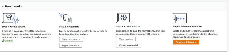
To get started with Amazon Lookout for Equipment, we create a dataset, ingest data, train a model, and run inference by setting up a scheduler. After going through these steps, we show you how you can quickly set up a human review process using Amazon A2I and retrain your model with augmented or human reviewed datasets.

In the accompanying Jupyter notebook, we walk you through the following steps:

1. Create a dataset in Amazon Lookout for Equipment.
2. Ingest data into the Amazon Lookout for Equipment dataset.
3. Train a model in Amazon Lookout for Equipment.
4. Run diagnostics on the trained model.
5. Create an inference scheduler in Amazon Lookout for Equipment to send a simulated stream of real-time requests.
6. Set up an Amazon A2I private human loop and review the predictions from Amazon Lookout for Equipment.
7. Retrain your model based on augmented datasets from Amazon A2I.

Architecture overview

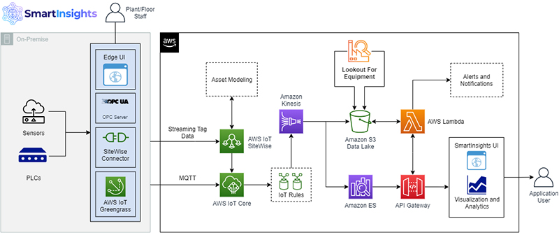
The following diagram illustrates our solution architecture.

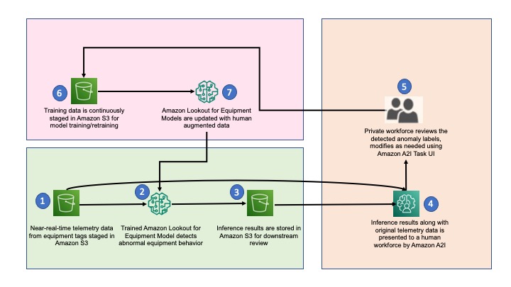
The workflow contains the following steps:

1. The architecture assumes that the inference pipeline is built and sensor data is periodically stored in the S3 path for inference inputs. These inputs are stored in CSV format with corresponding timestamps in the file name.
2. Amazon Lookout for Equipment wakes up at a prescribed frequency and processes the most recent file from the inference inputs Amazon Simple Storage Service (Amazon S3) path.
3. Inference results are stored in the inference outputs S3 path in JSON lines file format. The outputs also contain event diagnostics, which are used for root cause analysis.
4. When Amazon Lookout for Equipment detects an anomaly, the inference input and outputs are presented to the private workforce for validation via Amazon A2I.
5. A private workforce investigates and validates the detected anomalies and provides new anomaly labels. These labels are stored in a new S3 path.
6. Training data is also updated, along with the corresponding new labels, and is staged for subsequent model retraining.
7. After enough new labels are collected, a new Amazon Lookout for Equipment model is created, trained, and deployed. The retraining cycle can be repeated for continuous model retraining.

Prerequisites

Before you get started, complete the following steps to set up the Jupyter notebook:

1. Create a notebook instance in Amazon SageMaker.

Make sure your SageMaker notebook has the necessary AWS Identity and Access Management (IAM) roles and permissions mentioned in the prerequisite section of the notebook.

2. When the notebook is active, choose Open Jupyter.
3. On the Jupyter dashboard, choose New, and choose Terminal.
4. In the terminal, enter the following code:

cd SageMaker
git clone https://github.com/aws-samples/lookout-for-equipment-demo

5. First run the data preparation notebook – 1_data_preparation.ipynb
6. Then open the notebook for this blog – 3_integrate_l4e_and_a2i.ipynb

You’re now ready to run the following steps through the notebook cells. Run the setup environment step to set up the necessary Python SDKs and libraries that we use throughout the notebook.

7. Provide an AWS Region, create an S3 bucket, and provide details of the bucket in the following code cell:

REGION_NAME = '<your region>'
BUCKET = '<your bucket name>'
PREFIX = 'data/wind-turbine'

Analyze the dataset and create component metadata

In this section, we walk you through how you can preprocess the existing wind turbine data and ingest it for Amazon Lookout for Equipment. Please make sure to run the data preparation notebook prior to running the accompanying notebook for the blog to follow through all the steps in this post. You need a data schema for using your existing historical data with Amazon Lookout for Equipment. The data schema tells Amazon Lookout for Equipment what the data means. Because a data schema describes the data, its structure mirrors that of the data files of the components it describes.

All components must be described in the data schema. The data for each component is contained in a separate CSV file structured as shown in the data schema.

You store the data for each asset’s component in a separate CSV file using the following folder structure:

S3 bucket > Asset_name > Component 1 > Component1.csv

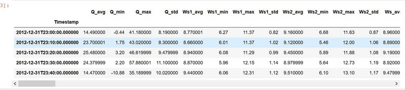
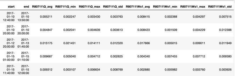
Go to the notebook section Pre-process and Load Datasets and run the following cell to inspect the data:

import pandas as pd
turbine_id = 'R80711'
df = pd.read_csv(f'../data/wind-turbine/interim/{turbine_id}.csv', index_col = 'Timestamp')
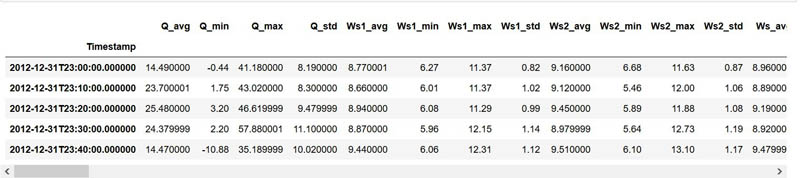
df.head()

The following screenshot shows our output.

Now we create components map to create a dataset expected by Amazon Lookout for Equipment for ingest. Run the notebook cells under the section Create the Dataset Component Map to create a component map and generate a CSV file for ingest.

Create the Amazon Lookout for Equipment dataset

We use Amazon Lookout for Equipment Create Dataset APIs to create a dataset and provide the component map we created in the previous step as an input. Run the following notebook cell to create a dataset:

ROLE_ARN = sagemaker.get_execution_role()
# REGION_NAME = boto3.session.Session().region_name
DATASET_NAME = 'wind-turbine-train-dsv2-PR'
MODEL_NAME = 'wind-turbine-PR-v1'

lookout_dataset = lookout.LookoutEquipmentDataset(
dataset_name=DATASET_NAME,
component_fields_map=DATASET_COMPONENT_FIELDS_MAP,
region_name=REGION_NAME,
access_role_arn=ROLE_ARN
)

pp = pprint.PrettyPrinter(depth=5)
pp.pprint(eval(lookout_dataset.dataset_schema))
lookout_dataset.create()

You get the following output:

Dataset "wind-turbine-train-dsv2-PR" does not exist, creating it...


{'DatasetName': 'wind-turbine-train-dsv2-PR',
 'DatasetArn': 'arn:aws:lookoutequipment:ap-northeast-2:<aws-account>:dataset/wind-turbine-train-dsv2-PR/8325802a-9bb7-48fb-804b-ab9f5b79f49d',
 'Status': 'CREATED',
 'ResponseMetadata': {'RequestId': '52dc754c-84da-4a8c-aaef-1908e4348837',
  'HTTPStatusCode': 200,
  'HTTPHeaders': {'x-amzn-requestid': '52dc754c-84da-4a8c-aaef-1908e4348837',
   'content-type': 'application/x-amz-json-1.0',
   'content-length': '203',
   'date': 'Thu, 25 Mar 2021 21:18:29 GMT'},
  'RetryAttempts': 0}}

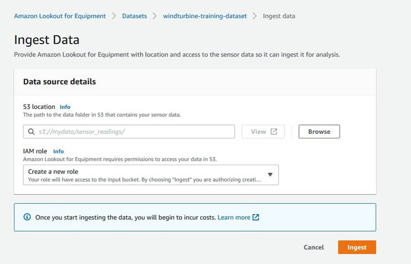
Alternatively, you can go to the Amazon Lookout for Equipment console to view the dataset.

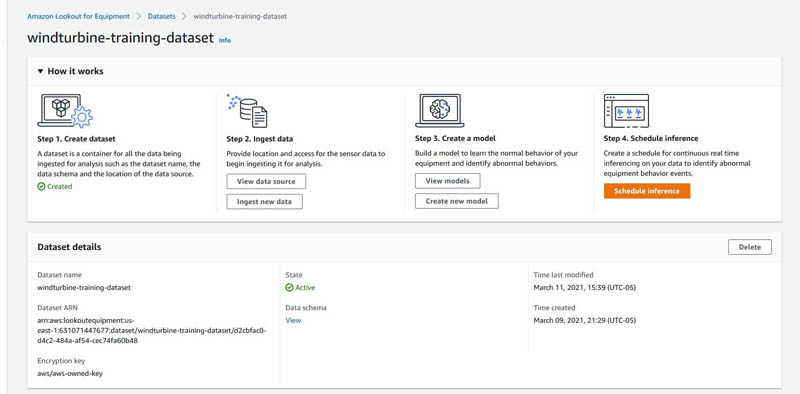
You can choose View under Data schema to view the schema of the dataset. You can choose Ingest new data to start ingesting data through the console, or you can use the APIs shown in the notebook to do the same using Python Boto3 APIs.

Run the notebook cells to ingest the data. When ingestion is complete, you get the following response:

=====Polling Data Ingestion Status=====

2021-03-25 21:18:45 |  IN_PROGRESS
2021-03-25 21:19:46 |  IN_PROGRESS
2021-03-25 21:20:46 |  IN_PROGRESS
2021-03-25 21:21:46 |  IN_PROGRESS
2021-03-25 21:22:46 |  SUCCESS

Now that we have preprocessed the data and ingested the data into Amazon Lookout for Equipment, we move on to the training steps. Alternatively, you can choose Ingest data.

Label your dataset using the SageMaker labeling workforce

If you don’t have an existing labeled dataset available to directly use with Amazon Lookout for Equipment, create a custom labeling workflow. This may be relevant in a use case in which, for example, a company wants to build a remote operating facility where alerts from various operations are sent to the central facility for the SMEs to review and update. For a sample crowd HTML template for your labeling UI, refer to our GitHub repository.

The following screenshot shows an example of what the sample labeling UI looks like.

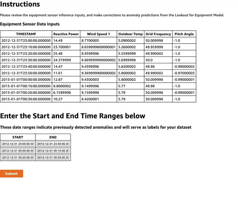
For this post, we use the labels that came with the dataset for training. If you want to use the label file you created for your actual training in the next step, you need to copy the label file to an S3 bucket and provide the location in the training configuration.

Create a model in Amazon Lookout for Equipment

We walk you through the following steps in this section:

• Prepare the model parameters and split data into test and train sets
• Train the model using Amazon Lookout for Equipment APIs
• Get diagnostics for the trained model

Prepare the model parameters and split the data

In this step, we split the datasets into test and train, prepare labels, and start the training using the notebook. Run the notebook code Split train and test to split the dataset into an 80/20 split for training and testing, respectively. Then run the prepare labels code and move on to setting up training config, as shown in the following code:

# Prepare the model parameters:
lookout_model = lookout.LookoutEquipmentModel(model_name=MODEL_NAME,
                                              dataset_name=DATASET_NAME,
                                              region_name=REGION_NAME)

# Set the training / evaluation split date:
lookout_model.set_time_periods(evaluation_start,
                               evaluation_end,
                               training_start,
                               training_end)

# Set the label data location:
lookout_model.set_label_data(bucket=BUCKET, 
                             prefix=PREFIX+'/labelled_data/',
                             access_role_arn=ROLE_ARN)

# This sets up the rate the service will resample the data before 
# training:
lookout_model.set_target_sampling_rate(sampling_rate='PT10M')

In the preceding code, we set up model training parameters such as time periods, label data, and target sampling rate for our model. For more information about these parameters, see CreateModel.

Train model

After setting these model parameters, you need to run the following train model API to start training your model with your dataset and the training parameters:

lookout_model.train()

You get the following response:

{'ModelArn': 'arn:aws:lookoutequipment:ap-northeast-2:<accountid>:model/wind-turbine-PR-v1/fac217a9-8855-4931-95f9-dd47f0af1ec5',
 'Status': 'IN_PROGRESS',
 'ResponseMetadata': {'RequestId': '3d385895-c62e-4126-9622-38f0ebed9715',
  'HTTPStatusCode': 200,
  'HTTPHeaders': {'x-amzn-requestid': '3d385895-c62e-4126-9622-38f0ebed9715',
   'content-type': 'application/x-amz-json-1.0',
   'content-length': '152',
   'date': 'Thu, 25 Mar 2021 21:27:05 GMT'},
  'RetryAttempts': 0}}

Alternatively, you can go to the Amazon Lookout for Equipment console and monitor the training after you create the model.

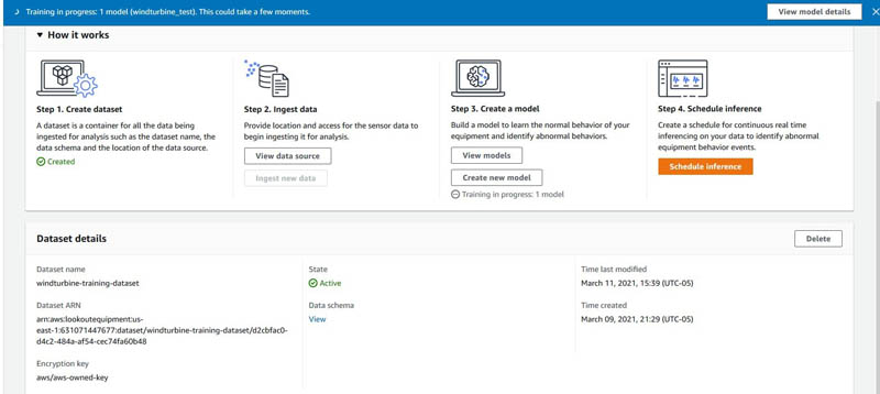
The sample turbine dataset we provide in our example has millions of data points. Training takes approximately 2.5 hours.

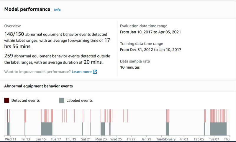
Evaluate the trained model

After a model is trained, Amazon Lookout for Equipment evaluates its performance and displays the results. It provides an overview of the performance and detailed information about the abnormal equipment behavior events and how well the model performed when detecting those. With the data and failure labels that you provided for training and evaluating the model, Amazon Lookout for Equipment reports how many times the model’s predictions were true positives. It also reports the average forewarning time across all true positives. Additionally, it reports the false positive results generated by the model, along with the duration of the non-event.

For more information about performance evaluation, see Evaluating the output.

Review training diagnostics

Run the following code to generate the training diagnostics. Refer to the accompanying notebook for the complete code block to run for this step.

LookoutDiagnostics = lookout.LookoutEquipmentAnalysis(model_name=MODEL_NAME, tags_df=df, region_name=REGION_NAME)
LookoutDiagnostics.set_time_periods(evaluation_start, evaluation_end, training_start, training_end)
predicted_ranges = LookoutDiagnostics.get_predictions()

The results returned show the percentage contribution of each feature towards the abnormal equipment prediction for the corresponding date range.

Create an inference scheduler in Amazon Lookout for Equipment

In this step, we show you how the CreateInferenceScheduler API creates a scheduler and starts it—this starts costing you right away. Scheduling an inference is setting up a continuous real-time inference plan to analyze new measurement data. When setting up the scheduler, you provide an S3 bucket location for the input data, assign it a delimiter between separate entries in the data, set an offset delay if desired, and set the frequency of inference. You must also provide an S3 bucket location for the output data. Run the following notebook section to run inference on the model to create an inference scheduler:

scheduler = lookout.LookoutEquipmentScheduler(
scheduler_name=INFERENCE_SCHEDULER_NAME,
model_name=MODEL_NAME_FOR_CREATING_INFERENCE_SCHEDULER,
region_name=REGION_NAME
)

scheduler_params = {
'input_bucket': INFERENCE_DATA_SOURCE_BUCKET,
'input_prefix': INFERENCE_DATA_SOURCE_PREFIX,
'output_bucket': INFERENCE_DATA_OUTPUT_BUCKET,
'output_prefix': INFERENCE_DATA_OUTPUT_PREFIX,
'role_arn': ROLE_ARN_FOR_INFERENCE,
'upload_frequency': DATA_UPLOAD_FREQUENCY,
'delay_offset': DATA_DELAY_OFFSET_IN_MINUTES,
'timezone_offset': INPUT_TIMEZONE_OFFSET,
'component_delimiter': COMPONENT_TIMESTAMP_DELIMITER,
'timestamp_format': TIMESTAMP_FORMAT
}

scheduler.set_parameters(**scheduler_params)

After you create an inference scheduler, the next step is to create some sample datasets for inference.

Prepare the inference data

Run through the notebook steps to prepare the inference data. Let’s load the tags description; this dataset comes with a data description file. From here, we can collect the list of components (subsystem column) if required. We use the tag metadata from the data descriptions as a point of reference for our interpretation. We use the tag names to construct a list that Amazon A2I uses. For more details, refer to the section Set up Amazon A2I to review predictions from Amazon Lookout for Equipment in this post.

To build our sample inference dataset, we extract the last 2 hours of data from the evaluation period of the original time series. Specifically, we create three CSV files containing simulated real-time tags for our turbine 10 minutes apart. These are all stored in Amazon S3 in the inference-a2i folder. Now that we’ve prepared the data, create the scheduler by running the following code:

create_scheduler_response = scheduler.create()

You get the following response:

===== Polling Inference Scheduler Status =====

Scheduler Status: PENDING
Scheduler Status: RUNNING

===== End of Polling Inference Scheduler Status =====

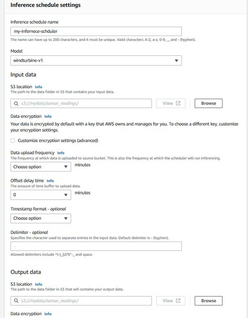
Alternatively, on the Amazon Lookout for Equipment console, go to the Inference schedule settings section of your trained model and set up a scheduler by providing the necessary parameters.

Get inference results

Run through the notebook steps List inference executions to get the run details from the schedule you created in the previous step. Wait 5–15 minutes for the scheduler to run its first inference. When it’s complete, we can use the ListInferenceExecution API for our current inference scheduler. The only mandatory parameter is the scheduler name.

You can also choose a time period for which you want to query inference runs. If you don’t specify it, all runs for an inference scheduler are listed. If you want to specify the time range, you can use the following code:

START_TIME_FOR_INFERENCE_EXECUTIONS = datetime.datetime(2010,1,3,0,0,0)END_TIME_FOR_INFERENCE_EXECUTIONS = datetime.datetime(2010,1,5,0,0,0)

This code means that the runs after 2010-01-03 00:00:00 and before 2010-01-05 00:00:00 are listed.

You can also choose to query for runs in a particular status, such as IN_PROGRESS, SUCCESS, and FAILED:

START_TIME_FOR_INFERENCE_EXECUTIONS = None
END_TIME_FOR_INFERENCE_EXECUTIONS = None
EXECUTION_STATUS = None

execution_summaries = []

while len(execution_summaries) == 0:
    execution_summaries = scheduler.list_inference_executions(
        start_time=START_TIME_FOR_INFERENCE_EXECUTIONS,
        end_time=END_TIME_FOR_INFERENCE_EXECUTIONS,
        execution_status=EXECUTION_STATUS
    )
    if len(execution_summaries) == 0:
        print('WAITING FOR THE FIRST INFERENCE EXECUTION')
        time.sleep(60)
        
    else:
        print('FIRST INFERENCE EXECUTEDn')
        break
            
execution_summaries

You get the following response:

{'ModelName': 'wind-turbine-PR-v1',
  'ModelArn': 'arn:aws:lookoutequipment:ap-northeast-2:<aws-account>:model/wind-turbine-PR-v1/fac217a9-8855-4931-95f9-dd47f0af1ec5',
  'InferenceSchedulerName': 'wind-turbine-scheduler-a2i-PR-v10',
  'InferenceSchedulerArn': 'arn:aws:lookoutequipment:ap-northeast-2:<aws-account>:inference-scheduler/wind-turbine-scheduler-a2i-PR-v10/e633c39d-a4f9-49f6-8248-7594349db2d0',
  'ScheduledStartTime': datetime.datetime(2021, 3, 29, 15, 35, tzinfo=tzlocal()),
  'DataStartTime': datetime.datetime(2021, 3, 29, 15, 30, tzinfo=tzlocal()),
  'DataEndTime': datetime.datetime(2021, 3, 29, 15, 35, tzinfo=tzlocal()),
  'DataInputConfiguration': {'S3InputConfiguration': {'Bucket': '<your s3 bucket>',
    'Prefix': 'data/wind-turbine/inference-a2i/input/'}},
  'DataOutputConfiguration': {'S3OutputConfiguration': {'Bucket': '<your s3 bucket>',
    'Prefix': 'data/wind-turbine/inference-a2i/output/'}},
  'CustomerResultObject': {'Bucket': '<your s3 bucket>',
   'Key': 'data/wind-turbine/inference-a2i/output/2021-03-29T15:30:00Z/results.jsonl'},
  'Status': 'SUCCESS'}]

Get actual prediction results

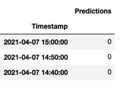
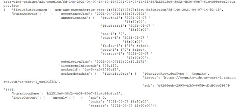
After each successful inference, a JSON file is created in the output location of your bucket. Each inference creates a new folder with a single results.jsonl file in it. You can run through this section in the notebook to read these files and display their content.

results_df

The following screenshot shows the results.

Stop the inference scheduler

Make sure to stop the inference scheduler; we don’t need it for the rest of the steps in this post. However, as part of your solution, the inference scheduler should be running to ensure real-time inference for your equipment continues. Run through this notebook section to stop the inference scheduler.

Set up Amazon A2I to review predictions from Amazon Lookout for Equipment

Now that inference is complete, let’s understand how to set up a UI to review the inference results and update it, so we can send it back to Amazon Lookout for Equipment for retraining the model. In this section, we show how to use the Amazon A2I custom task type to integrate with Amazon Lookout for Equipment through the walkthrough notebook to set up a human in the loop process. It includes the following steps:

• Create a human task UI
• Create a workflow definition
• Send predictions to Amazon A2I human loops
• Sign in to the worker portal and annotate Amazon Lookout for Equipment inference predictions

Follow the steps provided in the notebook to initialize Amazon A2I APIs. Make sure to set up the bucket name in the initialization block where you want your Amazon A2I output:

a2ibucket = '<your bucket>'

You also need to create a private workforce and provide a work team ARN in the initialize step.

On the SageMaker console, create a private workforce. After you create the private workforce, find the workforce ARN and enter the ARN in the notebook:

WORKTEAM_ARN = 'your private workforce team ARN'

Create the human task UI

You now create a human task UI resource, giving a UI template in liquid HTML. You can download the provided template and customize it. This template is rendered to the human workers whenever a human loop is required. For over 70 pre-built UIs, see the amazon-a2i-sample-task-uis GitHub repo. We also provide this template in our GitHub repo.

You can use this template to create a task UI either via the console or by running the following code in the notebook:

def create_task_ui():
 
    response = sagemaker_client.create_human_task_ui(
        HumanTaskUiName=taskUIName,
        UiTemplate={'Content': template})
    return response

Create a human review workflow definition

Workflow definitions allow you to specify the following:

• The worker template or human task UI you created in the previous step.
• The workforce that your tasks are sent to. For this post, it’s the private workforce you created in the prerequisite steps.
• The instructions that your workforce receives.

This post uses the Create Flow Definition API to create a workflow definition. Run the following cell in the notebook:

create_workflow_definition_response = sagemaker_client.create_flow_definition(
        FlowDefinitionName= flowDefinitionName,
        RoleArn=role,
        HumanLoopConfig= {
            "WorkteamArn": WORKTEAM_ARN,
            "HumanTaskUiArn": humanTaskUiArn,
            "TaskCount": 1,
            "TaskDescription": "Review the contents and select correct values as indicated",
            "TaskTitle": "Equipment Condition Review"
        },
        OutputConfig={
            "S3OutputPath" : OUTPUT_PATH
        }
    )
flowDefinitionArn = create_workflow_definition_response['FlowDefinitionArn'] 

Send predictions to Amazon A2I human loops

We create an item list from the Pandas DataFrame where we have the Amazon Lookout for Equipement output saved. Run the following notebook cell to create a list of items to send for review:

NUM_TO_REVIEW = 5 # number of line items to review
dftimestamp = sig_full_df['Timestamp'].astype(str).to_list()
dfsig001 = sig_full_df['Q_avg'].astype(str).to_list()
dfsig002 = sig_full_df['Ws1_avg'].astype(str).to_list()
dfsig003 = sig_full_df['Ot_avg'].astype(str).to_list()
dfsig004 = sig_full_df['Nf_avg'].astype(str).to_list()
dfsig046 = sig_full_df['Ba_avg'].astype(str).to_list()
sig_list = [{'timestamp': dftimestamp[x], 'reactive_power': dfsig001[x], 'wind_speed_1': dfsig002[x], 'outdoor_temp': dfsig003[x], 'grid_frequency': dfsig004[x], 'pitch_angle': dfsig046[x]} for x in range(NUM_TO_REVIEW)]
sig_list

Run the following code to create a JSON input for the Amazon A2I loop. This contains the lists that are sent as input to the Amazon A2I UI displayed to the human reviewers.

ip_content = {"signal": sig_list,
'anomaly': ano_list
}

Run the following notebook cell to call the Amazon A2I API to start the human loop:

import json
humanLoopName = str(uuid.uuid4())

start_loop_response = a2i.start_human_loop(
            HumanLoopName=humanLoopName,
            FlowDefinitionArn=flowDefinitionArn,
            HumanLoopInput={
                "InputContent": json.dumps(ip_content)
            }
        )

You can check the status of human loop by running the next cell in the notebook.

Annotate the results via the worker portal

Run the following notebook cell to get a login link to navigate to the private workforce portal:

workteamName = WORKTEAM_ARN[WORKTEAM_ARN.rfind('/') + 1:]
print("Navigate to the private worker portal and do the tasks. Make sure you've invited yourself to your workteam!")
print('https://' + sagemaker_client.describe_workteam(WorkteamName=workteamName)['Workteam']['SubDomain'])

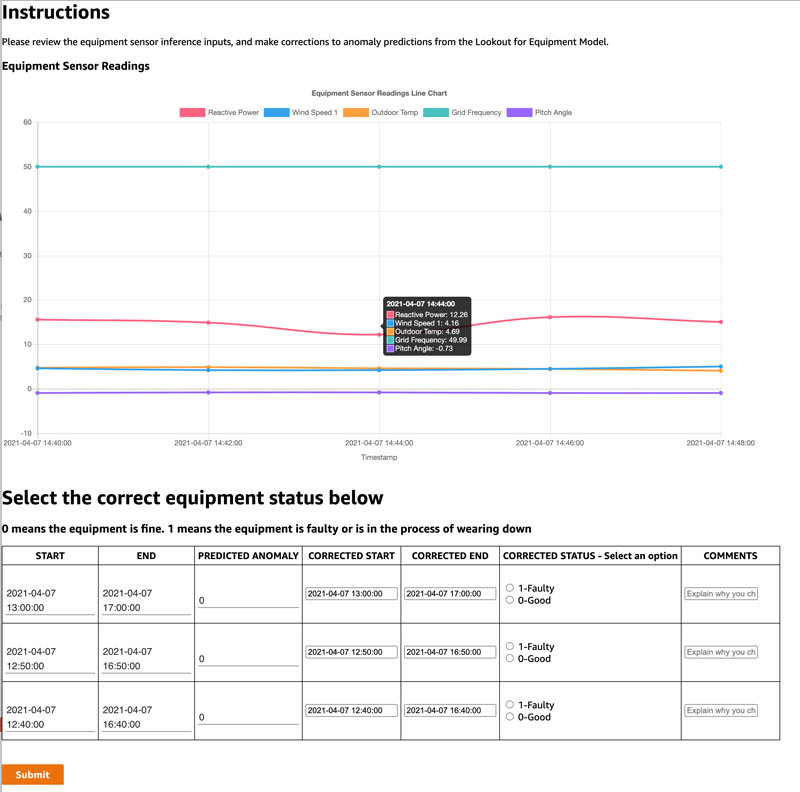
You’re redirected to the Amazon A2I console. Select the human review job and choose Start working. After you review the changes and make corrections, choose Submit.

You can evaluate the results store in Amazon S3.

Evaluate the results

When the labeling work is complete, your results should be available in the S3 output path specified in the human review workflow definition. The human answers are returned and saved in the JSON file. Run the notebook cell to get the results from Amazon S3:

import re
import pprint

pp = pprint.PrettyPrinter(indent=4)
json_output = ''
for resp in completed_human_loops:
    splitted_string = re.split('s3://' + a2ibucket  + '/', resp['HumanLoopOutput']['OutputS3Uri'])
    print(splitted_string[1])
    output_bucket_key = splitted_string[1]
    response = s3.get_object(Bucket=a2ibucket, Key=output_bucket_key)
    content = response["Body"].read()
    json_output = json.loads(content)
    pp.pprint(json_output)
    print('n')

You get a response with human reviewed answers and flow-definition. Refer to the notebook to get the complete response.

Model retraining based on augmented datasets from Amazon A2I

Now we take the Amazon A2I output, process it, and send it back to Amazon Lookout for Equipment to retrain our model based on the human corrections. Refer to the accompanying notebook for all the steps to complete in this section. Let’s look at the last few entries of our original label file:

labels_df = pd.read_csv(os.path.join(LABEL_DATA, 'labels.csv'), header=None)
labels_df[0] = pd.to_datetime(labels_df[0])
labels_df[1] = pd.to_datetime(labels_df[1])
labels_df.columns = ['start', 'end']
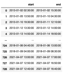
labels_df.tail()

The following screenshot shows the labels file.

Update labels with new date ranges

Now let’s update our existing labels dataset with the new labels we received from the Amazon A2I human review process:

faulty = False
a2i_lbl_df = labels_df
x = json_output['humanAnswers'][0]
row_df = pd.DataFrame(columns=['rownr'])
tslist = {}

# Let's first check if the users mark equipment as faulty and if so get those row numbers into a dataframe            
for i in json_output['humanAnswers']:
    print("checking equipment review...")
    x = i['answerContent']
    for idx, key in enumerate(x):
        if "faulty" in key:
            if str(x.get(key)).split(':')[1].lstrip().strip('}') == "True": # faulty equipment selected
                    faulty = True
                    row_df.loc[len(row_df.index)] = [key.split('-')[1]] 
                    print("found faulty equipment in row: " + key.split('-')[1])


# Now we will get the date ranges for the faulty choices                     
for idx,k in row_df.iterrows():
    x = json_output['humanAnswers'][0]
    strchk = "TrueStart"+k['rownr']
    endchk = "TrueEnd"+k['rownr']
    for i in x['answerContent']:
        if i == strchk:
            tslist[i] = x['answerContent'].get(i)
        if i == endchk:
            tslist[i] = x['answerContent'].get(i)

            
# And finally let's add it to our new a2i labels dataset
for idx,k in row_df.iterrows():
    x = json_output['humanAnswers'][0]
    strchk = "TrueStart"+k['rownr']
    endchk = "TrueEnd"+k['rownr']
    a2i_lbl_df.loc[len(a2i_lbl_df.index)] = [tslist[strchk], tslist[endchk]]

You get the following response:

checking equipment review...
found faulty equipment in row: 1
found faulty equipment in row: 2

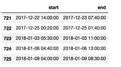
The following screenshot shows the updated labels file.

Let’s upload the updated labels data to a new augmented labels file:

a2i_label_s3_dest_path = f's3://{BUCKET}/{PREFIX}/augmented-labelled-data/labels.csv'
!aws s3 cp $a2i_label_src_fname $a2i_label_s3_dest_path

Update the training dataset with new measurements

We now update our original training dataset with the new measurement range based on what we got back from Amazon A2I. Run the following code to load the original dataset to a new DataFrame that we use to append our augmented data. Refer to the accompanying notebook for all the steps required.

turbine_id = 'R80711'
file = '../data/wind-turbine/final/training-data/'+turbine_id+'/'+turbine_id+'.csv'
newdf = pd.read_csv(file, index_col='Timestamp')
newdf.head()

The following screenshot shows our original training dataset snapshot.

Now we use the updated training dataset with the simulated inference data we created earlier, in which the human reviewers indicated that they found faulty equipment when running the inference. Run the following code to modify the index of the simulated inference dataset to reflect a 10-minute duration for each reading:

sig_full_df = sig_full_df.set_index('Timestamp')
tm = pd.to_datetime('2021-04-05 20:30:00')
print(tm)
new_index = pd.date_range(
start=tm,
periods=sig_full_df.shape[0],
freq='10min'
)
sig_full_df.index = new_index
sig_full_df.index.name = 'Timestamp'
sig_full_df = sig_full_df.reset_index()
sig_full_df['Timestamp'] = pd.to_datetime(sig_full_df['Timestamp'], errors='coerce')

Run the following code to append the simulated inference dataset to the original training dataset:

newdf = newdf.reset_index()
newdf = pd.concat([newdf,sig_full_df])

The simulated inference data with the recent timestamp is appended to the end of the training dataset. Now let’s create a CSV file and copy the data to the training channel in Amazon S3:

TRAIN_DATA_AUGMENTED = os.path.join(TRAIN_DATA,'augmented')
os.makedirs(TRAIN_DATA_AUGMENTED, exist_ok=True)
newdf.to_csv('../data/wind-turbine/final/training-data/augmented/'+turbine_id+'.csv')
!aws s3 sync $TRAIN_DATA_AUGMENTED s3://$BUCKET/$PREFIX/training_data/augmented

Now we update the components map with this augmented dataset, reload the data into Amazon Lookout for Equipment, and retrain this training model with this dataset. Refer to the accompanying notebook for the detailed steps to retrain the model.

Conclusion

In this post, we walked you through how to use Amazon Lookout for Equipment to train a model to detect abnormal equipment behavior with a wind turbine dataset, review diagnostics from the trained model, review the predictions from the model with a human in the loop using Amazon A2I, augment our original training dataset, and retrain our model with the feedback from the human reviews.

With Amazon Lookout for Equipment and Amazon A2I, you can set up a continuous prediction, review, train, and feedback loop to audit predictions and improve the accuracy of your models.

Please let us know what you think of this solution and how it applies to your industrial use case. Check out the GitHub repo for full resources to this post. Visit the webpages to learn more about Amazon Lookout for Equipment and Amazon Augmented AI. We look forward to hearing from you. Happy experimentation!

About the Authors 

 Dastan Aitzhanov is a Solutions Architect in Applied AI with Amazon Web Services. He specializes in architecting and building scalable cloud-based platforms with an emphasis on machine learning, internet of things, and big data-driven applications. When not working, he enjoys going camping, skiing, and spending time in the great outdoors with his family

Prem Ranga is an Enterprise Solutions Architect based out of Atlanta, GA. He is part of the Machine Learning Technical Field Community and loves working with customers on their ML and AI journey. Prem is passionate about robotics, is an Autonomous Vehicles researcher, and also built the Alexa-controlled Beer Pours in Houston and other locations.

Mona Mona is a Senior AI/ML Specialist Solutions Architect based out of Arlington, VA. She works with public sector customers, and helps them adopt machine learning on a large scale. She is passionate about NLP and ML explainability areas in AI/ML.

Baris Yasin is a Solutions Architect at AWS. He’s passionate about AI/ML & Analytics technologies and helping startup customers solve challenging business and technical problems with AWS.

Read More

As the modern factory becomes more connected, manufacturers are increasingly using a range of inputs (such as process data, audio, and visual) to increase their operational efficiency. Companies use this information to monitor equipment performance and anticipate failures using predictive maintenance techniques powered by machine learning (ML) and artificial intelligence (AI). Although traditional sensors built into the equipment can be informative, audio and visual inspection can also provide insights into the health of the asset. However, leveraging this data and gaining actionable insights can be highly manual and resource prohibitive.

Koch Ag & Energy Solutions, LLC (KAES) took the opportunity to collaborate with Amazon ML Solutions Lab to learn more about alternative acoustic anomaly detection solutions and to get another set of eyes on their existing solution.

The ML Solutions Lab team used the existing data collected by KAES equipment in the field for an in-depth acoustic data exploration. In collaboration with the lead data scientist at KAES, the ML Solutions Lab team engaged with an internal team at Amazon that had participated in the Detection and Classification of Acoustic Scenes and Events 2020 competition and won high marks for their efforts. After reviewing the documentation from Giri et al. (2020), the team presented some very interesting insights into the acoustic data:

• Industrial data is relatively stationary, so the recorded audio window size can be longer in duration
• Inference intervals could be increased from 1 second to 10–30 seconds.
• The sampling rates for the recorded sounds could be lowered and still retain the pertinent information

Furthermore, the team investigated two different approaches for feature engineering that KAES hadn’t previously explored. The first was an average-spectral featurizer; the second was an advanced deep learning based (VGGish network) featurizer. For this effort, the team didn’t need to use the classifier for the VGGish classes. Instead, they removed the top-level classifier layer and kept the network as a feature extractor. With this feature extraction approach, the network can convert audio input into high-level 128-dimensional embedding, which can be fed as input to another ML model. Compared to raw audio features, such as waveforms and spectrograms, this deep learning embedding is more semantically meaningful. The ML Solutions Lab team also designed an optimized API for processing all the audio files, which decreases the I/O time by more than 90%, and the overall processing time by around 70%.

Anomaly detection with Amazon Lookout for Equipment

To implement these solutions, the ML Solutions Lab team used Amazon Lookout for Equipment, a new service that helps to enable predictive maintenance. Amazon Lookout for Equipment uses AI to learn the normal operating patterns of industrial equipment and alert users to abnormal equipment behavior. Amazon Lookout for Equipment helps organizations take action before machine failures occur and avoid unplanned downtime.

Successfully implementing predictive maintenance depends on using the data collected from industrial equipment sensors, under their unique operating conditions, and then applying sophisticated ML techniques to build a custom model that can detect abnormal machine conditions before machine failures occur.

Amazon Lookout for Equipment analyzes the data from industrial equipment sensors to automatically train a specific ML model for that equipment with no ML expertise required. It learns the multivariate relationships between the sensors (tags) that define the normal operating modes of the equipment. With this service, you can reduce the number of manual data science steps and resource hours to develop a model. Furthermore, Amazon Lookout for Equipment uses the unique ML model to analyze incoming sensor data in near-real time to accurately identify early warning signs that could lead to machine failures with little or no manual intervention. This enables detecting equipment abnormalities with speed and precision, quickly diagnosing issues, taking action to reduce expensive downtime, and reducing false alerts.

With KAES, the ML Solutions Lab team developed a proof of concept pipeline that demonstrated the data ingestion steps for both sound and machine telemetry. The team used the telemetry data to identify the machine operating states and inform which audio data was relevant for training. For example, a pump at low speed has a certain auditory signature, whereas a pump at high speed may have a different auditory signature. The relationship between measurements like RPMs (speed) and the sound are key to understanding machine performance and health. The ML training time decreased from around 6 hours to less than 20 minutes when using Amazon Lookout for Equipment, which enabled faster model explorations.

This pipeline can serve as the foundation to build and deploy anomaly detection models for new assets. After sufficient data is ingested into the Amazon Lookout for Equipment platform, inference can begin and anomaly detections can be identified.

“We needed a solution to detect acoustic anomalies and potential failures of critical manufacturing machinery,” says Dave Kroening, IT Leader at KAES. “Within a few weeks, the experts at the ML Solutions Lab worked with our internal team to develop an alternative, state-of-the-art, deep neural net embedding sound featurization technique and a prototype for acoustic anomaly detection. We were very pleased with the insight that the ML Solutions Lab team provided us regarding our data and educating us on the possibilities of using Amazon Lookout for Equipment to build and deploy anomaly detection models for new assets.”

By merging the sound data with the machine telemetry data and then using Amazon Lookout for Equipment, we can derive important relationships between the telemetry data and the acoustic signals. We can learn the normal healthy operating conditions and healthy sounds in varying operating modes.

If you’d like help accelerating the use of ML in your products and services, please contact the ML Solutions Lab.

About the Authors

Michael Robinson is a Lead Data Scientist at Koch Ag & Energy Solutions, LLC (KAES). His work focuses on computer vision, acoustic, and data engineering. He leverages technical knowledge to solve unique challenges for KAES. In his spare time, he enjoys golfing, photography and traveling.

Dave Kroening is an IT Leader with Koch Ag & Energy Solutions, LLC (KAES). His work focuses on building out a vision and strategy for initiatives that can create long term value. This includes exploring, assessing, and developing opportunities that have a potential to disrupt the Operating capability within KAES. He and his team also help to discover and experiment with technologies that can create a competitive advantage. In his spare time he enjoys spending time with his family, snowboarding, and racing.

Mehdi Noori is a Data Scientist at the Amazon ML Solutions Lab, where he works with customers across various verticals, and helps them to accelerate their cloud migration journey, and to solve their ML problems using state-of-the-art solutions and technologies. Mehdi attended MIT as a postdoctoral researcher and obtained his Ph.D. in Engineering from UCF.

Xin Chen is a senior manager at Amazon ML Solutions Lab, where he leads the Automotive Vertical and helps AWS customers across different industries identify and build machine learning solutions to address their organization’s highest return-on-investment machine learning opportunities. Xin obtained his Ph.D. in Computer Science and Engineering from the University of Notre Dame.

Yunzhi Shi is a data scientist at the Amazon ML Solutions Lab where he helps AWS customers address business problems with AI and cloud capabilities. Recently, he has been building computer vision, search, and forecast solutions for customers from various industrial verticals. Yunzhi obtained his Ph.D. in Geophysics from the University of Texas at Austin.

Dan Volk is a Data Scientist at Amazon ML Solutions Lab, where he helps AWS customers across various industries accelerate their AI and cloud adoption. Dan has worked in several fields including manufacturing, aerospace, and sports and holds a Masters in Data Science from UC Berkeley.

Brant Swidler is the Technical Product Manager for Amazon Lookout for Equipment. He focuses on leading product development including data science and engineering efforts. Brant comes from an Industrial background in the oil and gas industry and has a B.S. in Mechanical and Aerospace Engineering from Washington University in St. Louis and an MBA from the Tuck school of business at Dartmouth.

Read More

AWS DeepRacer is the fastest way to get rolling with machine learning, giving developers the chance to learn ML hands-on with a 1/18th scale autonomous car, 3D virtual racing simulator, and the world’s largest global autonomous car racing league. With the 2021 AWS DeepRacer League Virtual Circuit now underway, developers have five times more opportunities to win physical prizes, such as exclusive AWS DeepRacer merchandise, AWS DeepRacer Evo devices, and even an expenses paid trip to AWS re:Invent 2021 to compete in the AWS DeepRacer Championship Cup.

To win physical prizes, show us your skills by racing in one of the AWS monthly qualifiers, becoming a Pro by finishing in the top 10% of an Open race leaderboard, or qualifying for the championship by winning a monthly Pro division finale. To make ML more fun and accessible to every developer, the AWS DeepRacer League is taking prizing a step further and introducing new digital car customizations for every participant in the league. For each month that you participate, you’ll earn a reward exclusive to that race and division. After all, if your ML model is getting rewarded, shouldn’t you get rewarded too?

Digital rewards: Collect them all and showcase your collection

Digital rewards are unique cars, paint jobs, and body kits that are stored in a new section of the AWS DeepRacer console: your racer profile. Unlocking a new reward is like giving your model the West Coast Customs car treatment. While X to the Z might be famous for kitting out your ride in the streets, A to the Z is here to hook you up in the virtual simulator!

No two rewards are exactly alike, and each month will introduce new rewards to be earned in each racing division to add to your collection. You’ll need to race every month to collect all of the open division digital rewards in your profile. If you advance to the Pro division, you’ll unlock twice the rewards, with an additional Pro division reward each month that’s only available to the fastest in the league.

If you participated in the March 2021 races, you’ll see some special deliveries dropping into your racer profile starting today. Open division racers will receive the white box van, and Pro division racers will receive both the white box van and the Pro Exclusive AWS DeepRacer Van. Despite their size, they’re just as fast as any other vehicle you race on the console—they’re merely skins and don’t change the agent’s capabilities or performance.

But that’s not all—AWS DeepRacer will keep the rewards coming with surprise limited edition rewards throughout the season for specific racing achievements and milestones. But you’ll have to keep racing to find them! When it’s time to celebrate, the confetti will fall! The next time you log in and access your racer profile, you’ll see the celebration to commemorate your achievement. After a new digital reward is added to your racer profile, you can choose the reward to open your garage and start personalizing your car and action space, or assign it to any existing model in your garage using the Mod vehicle feature.

When you select that model to race in the league, you’ll see your customized vehicle in your race evaluation video. You can also head over to the race leaderboard to watch other racer’s evaluations and check out which customizations they’re using for their models to size up the competition.

Customize your racer profile and avatar

While new digital rewards allow you to customize your car on the track, the new Your racer profile page allows you to customize your personal appearance across the AWS DeepRacer console. With the new avatar tool, you can select from a variety of options to replicate your real-life style or try out a completely new appearance to showcase your personality. Your racer profile also allows you to designate your country, which adds a flag to your avatar and in-console live races, giving you the opportunity to represent your region and see where other competitors are racing from all over the globe.

Your avatar appears on each race leaderboard page for you to see, and if you’re on top of the leaderboard, everyone can see your avatar in first position, claiming victory! If you qualify to participate in a live race such as the monthly Pro division finale, your avatar is also featured each time you’re on the track. In addition to housing the avatar tool and your digital rewards, the Your racer profile page also provides useful stats such as your division, the number of races you have won, and how long you have been racing in the AWS DeepRacer League.

Get rolling today

The April 2021 races are just getting underway in the Virtual Circuit. Head over to the AWS DeepRacer League today to get rolling, or sign in to the AWS DeepRacer console to start customizing your avatar and collecting digital rewards!

To see the new avatars in action, tune into the AWS DeepRacer League LIVE Pro Finale at 5:30pm PST, the second Thursday of every month on the AWS Twitch channel. The first race will take place on April 8th.

About the Author

Joe Fontaine is the Marketing Program Manager for AWS AI/ML Developer Devices. He is passionate about making machine learning more accessible to all through hands-on educational experiences. Outside of work he enjoys freeride mountain biking, aerial cinematography, and exploring the wilderness with his dogs. He is proud to be a recent inductee to the “rad dads” club.

Read More

Machine downtime has a dramatic impact on your operational efficiency. Unexpected machine downtime is even worse. Detecting industrial equipment issues at an early stage and using that data to inform proper maintenance can give your company a significant increase in operational efficiency.

Customers see value in detecting abnormal behavior in industrial equipment to improve maintenance lifecycles. However, implementing advanced maintenance approaches has multiple challenges. One major challenge is the plethora of data recorded from sensors and log information, as well as managing equipment and site metadata. These different forms of data may either be inaccessible or spread across disparate systems that can impede access and processing. After this data is consolidated, the next step is gaining insights to prioritize the most operationally efficient maintenance strategy.

A range of data processing tools exist today, but most require significant manual effort to implement or maintain, which acts as a barrier to use. Furthermore, managing advanced analytics such as machine learning (ML) requires either in-house or external data scientists to manage models for each type of equipment. This can lead to a high cost of implementation and can be daunting for operators that manage hundreds or thousands of sensors in a refinery or hundreds of turbines on a wind farm.

Real-time data capture and monitoring of your IoT assets with TensorIoT

TensorIoT, an AWS Advanced Consulting Partner, is no stranger to the difficulties companies face when looking to harness their data to improve their business practices. TensorIoT creates products and solutions to help companies benefit from the power of ML and IoT.

“Regardless of size or industry, companies are seeking to achieve greater situational awareness, gain actionable insight, and make more confident decisions,” says John Traynor, TensorIoT VP of Products.

For industrial customers, TensorIoT is adept at integrating sensors and machine data with AWS tools into a holistic system that keeps operators informed about the status of their equipment at all times. TensorIoT uses AWS IoT Greengrass with AWS IoT SiteWise and other AWS Cloud services to help clients collect data from both direct equipment measurements and add-on sensors through connected devices to measure factors such as humidity, temperature, pressure, power, and vibration, giving a holistic view of machine operation. To help businesses gain increased understanding of their data and processes, TensorIoT created SmartInsights, a product that incorporates data from multiple sources for analysis and visualization. Clear visualization tools combined with advanced analytics means that the assembled data is easy to understand and actionable for users. This is seen in the following screenshot, which shows the specific site where an anomaly occurred and a ranking based on production or process efficiency.

TensorIoT built the connectivity to get the data ingestion into Amazon Lookout for Equipment (an industrial equipment monitoring service that detects abnormal equipment behavior) for analysis, and then used SmartInsights as the visualization tool for users to act on the outcome. Whether an operational manager wants to visualize the health of the asset or provide an automated push notification sent to maintenance teams such as an alarm or Amazon Simple Notification Service (Amazon SNS) message, SmartInsights keeps industrial sites and factory floors operating at peak performance for even the most complex device hierarchies. Powered by AWS, TensorIoT helps companies rapidly and precisely detect equipment abnormalities, diagnose issues, and take immediate action to reduce expensive downtime.

Simplify machine learning with Amazon Lookout for Equipment

ML offers industrial companies the ability to automatically discover new insights from data that is being collected across systems and equipment types. In the past, however, industrial ML-enabled solutions such as equipment condition monitoring have been reserved for the most critical or expensive assets, due to the high cost of developing and managing the required models. Traditionally, a data scientist needed to go through dozens of steps to build an initial model for industrial equipment monitoring that can detect abnormal behavior. Amazon Lookout for Equipment automates these traditional data science steps to open up more opportunities for a broader set of equipment than ever before. Amazon Lookout for Equipment reduces the heavy lifting to create ML algorithms so you can take advantage of industrial equipment monitoring to identify anomalies, and gain new actionable insights that help you improve your operations and avoid downtime.

Historically, ML models can also be complex to manage due to changing or new operations. Amazon Lookout for Equipment is making it easier and faster to get feedback from the engineers closest to the equipment by enabling direct feedback and iteration of these models. That means that a maintenance engineer can prioritize which insights are the most important to detect based on current operations, such as process, signal, or equipment issues. Amazon Lookout for Equipment enables the engineer to label these events to continue to refine and prioritize so the insights stay relevant over the life of the asset.

Combining TensorIoT and Amazon Lookout for Equipment has never been easier

To delve deeper into how to visualize near real-time insights gained from Amazon Lookout for Equipment, let’s explore the process. It’s important to have historic and failure data so we can train the model to learn what patterns occur before failure. When trained, the model can create inferences about pending events from new, live data from that equipment. This, historically, is a time-consuming barrier to adoption because each piece of equipment requires separate training due to its unique operation and is solved through Amazon Lookout for Equipment and visualized by SmartInsights.

For our example, we start by identifying a suitable dataset where we have sensor and other operational data from a piece of equipment, as well as historic data about when the equipment has been operating outside of specifications or has failed, if available.

To demonstrate how to use Amazon Lookout for Equipment and visualize results in near real time in SmartInsights, we used a publicly available set of wind turbine data. Our dataset from the La Haute Borne wind farm spanned several hundred thousand rows and over 100 columns of data from a variety of sensors on the equipment. Data included the rotor speed, pitch angle, generator bearing temperatures, gearbox bearing temperatures, oil temperature, multiple power measurements, wind speed and direction, outdoor temperature, and more. The maximum, average, and other statistical characteristics were also stored for each data point.

The following table is a subset of the columns used in our analysis.

Using Amazon Lookout for Equipment consists of three stages: ingestion, training, and inference (or detection). After the model is trained with available historical data, inference can happen automatically on a selected time interval, such as every 5 minutes or 1 hour.

First, let’s look at the Amazon Lookout for Equipment side of the process. In this example, we trained using historic data and evaluated the model against 1 year of historic data. Based on these results, 148 of the 150 events were detected with an average forewarning time of 18 hours.

For each of the events, a diagnostic of the key contributing sensors is given to support evaluation of the root cause, as shown in the following screenshot.

SmartInsights provides visualization of data from each asset and incorporates the events from Amazon Lookout for Equipment. SmartInsights can then pair the original measurements with the anomalies identified by Amazon Lookout for Equipment using the common timestamp. This allows SmartInsights to show measurements and anomalies on a common timescale and gives the operator context to these events. In the following graphical representation, a green bar is overlaid on top of the anomalies. You can deep dive by evaluating the diagnostics against the asset to determine when and how to respond to the event.

With the wind turbine data that was used in our example, SmartInsights provided visual evidence of the events with forewarning based on results for Amazon Lookout for Equipment. In a production environment, the prediction could create a notification or alert to operating personnel or trigger a work order to be created in another application to dispatch personnel to take corrective action before failure.

SmartInsights supports triggering alerts in response to certain conditions. For example, you can configure SmartInsights to send a message to a Slack channel or send a text message. Because SmartInsights is built on AWS, the notification endpoint can be any destination supported by Amazon SNS. For example, the following view of SmartInsights on a mobile device contains a list of alerts that have been triggered within a certain time window, to which a SmartInsights user can subscribe.

The following architecture diagram shows how Amazon Lookout for Equipment is used with SmartInsights. For many applications, Amazon Lookout for Equipment provides an accelerated path to anomaly detection without the need to hire a data scientist and meet business return on investment.

Maximize uptime, increase safety, and improve machine efficiency

Condition-based maintenance is beneficial for your business on a multitude of levels:

• Maximized uptime – When maintenance events are predicted, you decide the optimal scheduling to minimize the impact on your operational efficiency.
• Increased safety – Condition-based maintenance ensures that your equipment remains in safe operating conditions, which protects your operators and your machinery by catching issues before they become problems.
• Improved machine efficiency – As your machines undergo normal wear and tear, their efficiency decreases. Condition-based maintenance keeps your machines in optimal conditions and extends the lifespan of your equipment.

Conclusion

Even before the release of Amazon Lookout for Equipment, TensorIoT helped industrial manufacturers innovate their machinery through the implementation of modern architectures, sensors for legacy augmentation, and ML to make the newly acquired data intelligible and actionable. With Amazon Lookout for Equipment and TensorIoT solutions, TensorIoT helps make your assets even smarter.

To explore how you can use Amazon Lookout for Equipment with SmartInsights to more rapidly gain insight into pending equipment failures and reduce downtime, get in touch with TensorIoT via contact@tensoriot.com.

Details on how to start using Amazon Lookout for Equipment are available on the webpage.

About the Authors

Alicia Trent is a Worldwide Business Development Manager at Amazon Web Services. She has 15 years of experience in Technology across industrial sectors and is a graduate of the Georgia Institute of Technology, where she earned a BS degree in chemical and biomolecular engineering, and an MS degree in mechanical engineering.

Dastan Aitzhanov is a Solutions Architect in Applied AI with Amazon Web Services. He specializes in architecting and building scalable cloud-based platforms with an emphasis on Machine Learning, Internet of Things, and Big Data driven applications. When not working, he enjoys going camping, skiing, and just spending time in the great outdoors with his family.

Nicholas Burden is a Senior Technical Evangelist at TensorIoT, where he focuses on translating complex technical jargon into digestible information. He has over a decade of technical writing experience and a Master’s in Professional Writing from USC. Outside of work, he enjoys tending to an ever-growing collection of houseplants and spending time with pets and family.

Read More

Deep learning is at the forefront of most machine learning (ML) implementations across a broad set of business verticals. Driven by the highly flexible nature of neural networks, the boundary of what is possible has been pushed to a point where neural networks can outperform humans in a variety of tasks, such as object detection tasks in the context of computer vision (CV) problems.

Object detection, which is one type of CV task, has many applications in various fields like medicine, retail, or agriculture. For example, retail businesses want to be able to detect stock keeping units (SKUs) in store shelf images to analyze buyer trends or identify when product restock is necessary. Object detection models allow you to implement these diverse use cases and automate your in-store operations.

In this post, we discuss Detectron2, an object detection and segmentation framework released by Facebook AI Research (FAIR), and its implementation on Amazon SageMaker to solve a dense object detection task for retail. This post includes an associated sample notebook, which you can run to demonstrate all the features discussed in this post. For more information, see the GitHub repository.

Toolsets used in this solution

To implement this solution, we use Detectron2, PyTorch, SageMaker, and the public SKU-110K dataset.

Detectron2

Detectron2 is a ground-up rewrite of Detectron that started with maskrcnn-benchmark. The platform is now implemented in PyTorch. With a new, more modular design, Detectron2 is flexible and extensible, and provides fast training on single or multiple GPU servers. Detectron2 includes high-quality implementations of state-of-the-art object detection algorithms, including DensePose, panoptic feature pyramid networks, and numerous variants of the pioneering Mask R-CNN model family also developed by FAIR. Its extensible design makes it easy to implement cutting-edge research projects without having to fork the entire code     base.

PyTorch

PyTorch is an open-source, deep learning framework that makes it easy to develop ML models and deploy them to production. With PyTorch’s TorchScript, developers can seamlessly transition between eager mode, which performs computations immediately for easy development, and graph mode, which creates computational graphs for efficient implementations in production environments. PyTorch also offers distributed training, deep integration into Python, and a rich ecosystem of tools and libraries, which makes it popular with researchers and engineers.

An example of that rich ecosystem of tools is TorchServe, a recently released model-serving framework for PyTorch that helps deploy trained models at scale without having to write custom code. TorchServe is built and maintained by AWS in collaboration with Facebook and is available as part of the PyTorch open-source project. For more information, see the TorchServe GitHub repo and Model Server for PyTorch Documentation.

Amazon SageMaker

SageMaker is a fully managed service that provides every developer and data scientist with the ability to build, train, and deploy ML models quickly. SageMaker removes the heavy lifting from each step of the ML process to make it easier to develop high-quality models.

Dataset

For our use case, we use the SKU-110 dataset introduced by Goldman et al. in the paper “Precise Detection in Densely Packed Scenes” (Proceedings of 2019 conference on Computer Vision and Patter Recognition). This dataset contains 11,762 images of store shelves from around the world. Researchers use this dataset to test object detection algorithms on dense scenes. The term density here refers to the number of objects per image. The average number of items per image is 147.4, which is 19 times more than the COCO dataset. Moreover, the images contain multiple identical objects grouped together that are challenging to separate. The dataset contains bounding box annotation on SKUs. The categories of product aren’t distinguished because the bounding box labels only indicate the presence or absence of an item.

Introduction to Detectron2

Detectron2 is FAIR’s next generation software system that implements state-of-the-art object detection algorithms. It’s a ground-up rewrite of the previous version, Detectron, and it originates from maskrcnn-benchmark. The following screenshot is an example of the high-level structure of the Detectron2 repo, which will make more sense when we explore configuration files and network architectures later in this post.

For more information about the general layout of computer vision and deep learning architectures, see A Survey of the Recent Architectures of Deep Convolutional Neural Networks.

Additionally, if this is your first introduction to Detectron2, see the official documentation to learn more about the feature-rich capabilities of Detectron2. For the remainder of this post, we solely focus on implementation details pertaining to deploying Detectron2-powered object detection on SageMaker rather than discussing the underlying computer vision-specific theory.

Update the SageMaker role

To build custom training and serving containers, you need to attach additional Amazon Elastic Container Registry (Amazon ECR) permissions to your SageMaker AWS Identity and Access Management (IAM) role. You can use an AWS-authored policy (such as AmazonEC2ContainerRegistryPowerUser) or create your own custom policy. For more information, see How Amazon SageMaker Works with IAM.

Update the dataset

Detectron2 includes a set of utilities for data loading and visualization. However, you need to register your custom dataset to use Detectron2’s data utilities. You can do this by using the function register_dataset in the catalog.py file from the GitHub repo. This function iterates on the training, validation, and test sets. At each iteration, it calls the function aws_file_mode, which returns a list of annotations given the path to the folder that contains the images and the path to the augmented manifest file that contains the annotations. Augmented manifest files are the output format of Amazon SageMaker Ground Truth bounding box jobs. You can reuse the code associated with this post on your own data labeled for object detection with Ground Truth.

Let’s prepare the SKU-110K dataset so that training, validation, and test images are in dedicated folders, and the annotations are in augmented manifest file format. First, import the required packages, define the S3 bucket, and set up the SageMaker session:

from pathlib import Path
from urllib import request
import tarfile
from typing import Sequence, Mapping, Optional
from tqdm import tqdm
from datetime import datetime
import tempfile
import json

import pandas as pd
import numpy as np
import boto3
import sagemaker

bucket = "my-bucket" # TODO: replace with your bucker
prefix_data = "detectron2/data"
prefix_model = "detectron2/training_artefacts"
prefix_code = "detectron2/model"
prefix_predictions = "detectron2/predictions"
local_folder = "cache"

sm_session = sagemaker.Session(default_bucket=bucket)
role = sagemaker.get_execution_role()

Then, download the dataset:

sku_dataset = ("SKU110K_fixed", "http://trax-geometry.s3.amazonaws.com/cvpr_challenge/SKU110K_fixed.tar.gz")

if not (Path(local_folder) / sku_dataset[0]).exists():
    compressed_file = tarfile.open(fileobj=request.urlopen(sku_dataset[1]), mode="r|gz")
    compressed_file.extractall(path=local_folder)
else:
    print(f"Using the data in `{local_folder}` folder")
path_images = Path(local_folder) / sku_dataset[0] / "images"
assert path_images.exists(), f"{path_images} not found"

prefix_to_channel = {
    "train": "training",
    "val": "validation",
    "test": "test",
}
for channel_name in prefix_to_channel.values():
    if not (path_images.parent / channel_name).exists():
        (path_images.parent / channel_name).mkdir()

for path_img in path_images.iterdir():
    for prefix in prefix_to_channel:
        if path_img.name.startswith(prefix):
            path_img.replace(path_images.parent / prefix_to_channel[prefix] / path_img.name)

Next, upload the image files to Amazon Simple Storage Service (Amazon S3) using the utilities from the SageMaker Python SDK:

channel_to_s3_imgs = {}

for channel_name in prefix_to_channel.values():
    inputs = sm_session.upload_data(
        path=str(path_images.parent / channel_name),
        bucket=bucket,
        key_prefix=f"{prefix_data}/{channel_name}"
    )
    print(f"{channel_name} images uploaded to {inputs}")
    channel_to_s3_imgs[channel_name] = inputs

SKU-110k annotations are stored in CSV files. The following function converts the annotations to JSON lines (refer to the GitHub repo to see the implementation):

def create_annotation_channel(
    channel_id: str, path_to_annotation: Path, bucket_name: str, data_prefix: str,
    img_annotation_to_ignore: Optional[Sequence[str]] = None
) -> Sequence[Mapping]:
    r"""Change format from original to augmented manifest files

    Parameters
    ----------
    channel_id : str
        name of the channel, i.e. training, validation or test
    path_to_annotation : Path
        path to annotation file
    bucket_name : str
        bucket where the data are uploaded
    data_prefix : str
        bucket prefix
    img_annotation_to_ignore : Optional[Sequence[str]]
        annotation from these images are ignore because the corresponding images are corrupted, default to None

    Returns
    -------
    Sequence[Mapping]
        List of json lines, each lines contains the annotations for a single. This recreates the
        format of augmented manifest files that are generated by Amazon SageMaker GroundTruth
        labeling jobs
    """
    …

channel_to_annotation_path = {
    "training": Path(local_folder) / sku_dataset[0] / "annotations" / "annotations_train.csv",
    "validation": Path(local_folder) / sku_dataset[0] / "annotations" / "annotations_val.csv",
    "test": Path(local_folder) / sku_dataset[0] / "annotations" / "annotations_test.csv",
}
channel_to_annotation = {}

for channel in channel_to_annotation_path:
    annotations = create_annotation_channel(
        channel,
        channel_to_annotation_path[channel],
        bucket,
        prefix_data,
        CORRUPTED_IMAGES[channel]
    )
    print(f"Number of {channel} annotations: {len(annotations)}")
    channel_to_annotation[channel] = annotations

Finally, upload the manifest files to Amazon S3:

def upload_annotations(p_annotations, p_channel: str):
    rsc_bucket = boto3.resource("s3").Bucket(bucket)
    
    json_lines = [json.dumps(elem) for elem in p_annotations]
    to_write = "n".join(json_lines)

    with tempfile.NamedTemporaryFile(mode="w") as fid:
        fid.write(to_write)
        rsc_bucket.upload_file(fid.name, f"{prefix_data}/annotations/{p_channel}.manifest")

for channel_id, annotations in channel_to_annotation.items():
    upload_annotations(annotations, channel_id)

Visualize the dataset

Detectron2 provides toolsets to inspect datasets. You can visualize the dataset input images and their ground truth bounding boxes. First, you need to add the dataset to the Detectron2 catalog:

import random
from typing import Sequence, Mapping
import cv2
from matplotlib import pyplot as plt
from detectron2.data import DatasetCatalog, MetadataCatalog
from detectron2.utils.visualizer import Visualizer
# custom code
from datasets.catalog import register_dataset, DataSetMeta

ds_name = "sku110k"
metadata = DataSetMeta(name=ds_name, classes=["SKU",])
channel_to_ds = {"test": ("data/test/", "data/test.manifest")}
register_dataset(
    metadata=metadata, label_name="sku", channel_to_dataset=channel_to_ds,
)

You can now plot annotations on an image as follows:

dataset_samples: Sequence[Mapping] = DatasetCatalog.get(f"{ds_name}_test")
sample = random.choice(dataset_samples)
fname = sample["file_name"]
print(fname)
img = cv2.imread(fname)
visualizer = Visualizer(
    img[:, :, ::-1], metadata=MetadataCatalog.get(f"{ds_name}_test"), scale=1.0
)
out = visualizer.draw_dataset_dict(sample)

plt.imshow(out.get_image())
plt.axis("off")
plt.tight_layout()
plt.show()

The following picture shows an example of ground truth bounding boxes on a test image.

Distributed training on Detectron2

You can use Docker containers with SageMaker to train Detectron2 models. In this post, we describe how you can run distributed Detectron2 training jobs for a larger number of iterations across multiple nodes and GPU devices on a SageMaker training cluster.

The process includes the following steps:

1. Create a training script capable of running and coordinating training tasks in a distributed environment.
2. Prepare a custom Docker container with configured training runtime and training scripts.
3. Build and push the training container to Amazon ECR.
4. Initialize training jobs via the SageMaker Python SDK.

Prepare the training script for the distributed cluster

The sku-100k folder contains the source code that we use to train the custom Detectron2 model. The script training.py is the entry point of the training process. The following sections of the script are worth discussing in detail:

• __main__ guard – The SageMaker Python SDK runs the code inside the main guard when used for training. The train function is called with the script arguments.
• _parse_args() – This function parses arguments from the command line and from the SageMaker environments. For example, you can choose which model to train among Faster-RCNN and RetinaNet. The SageMaker environment variables define the input channel locations and where the model artifacts are stored. The number of GPUs and the number of hosts define the properties of the training cluster.
• train() – We use the Detectron2 launch utility to start training on multiple nodes.
• _train_impl()– This is the actual training script, which is run on all processes and GPU devices. This function runs the following steps:
  • Register the custom dataset to Detectron2’s catalog.
  • Create the configuration node for training.
  • Fit the training dataset to the chosen object detection architecture.
  • Save the training artifacts and run the evaluation on the test set if the current node is the primary.

Prepare the training container

We build a custom container with the specific Detectron2 training runtime environment. As a base image, we use the latest SageMaker PyTorch container and further extend it with Detectron2 requirements. We first need to make sure that we have access to the public Amazon ECR (to pull the base PyTorch image) and our account registry (to push the custom container). The following example code shows how to log in to both registries prior to building and pushing your custom containers:

# loging to Sagemaker ECR with Deep Learning Containers
!aws ecr get-login-password --region us-east-2 | docker login --username AWS --password-stdin 763104351884.dkr.ecr.us-east-2.amazonaws.com
# loging to your private ECR
!aws ecr get-login-password --region us-east-2 | docker login --username AWS --password-stdin <YOUR-ACCOUNT-ID>.dkr.ecr.us-east-2.amazonaws.com

After you successfully authenticate with Amazon ECR, you can build the Docker image for training. This Dockerfile runs the following instructions:

1. Define the base container.
2. Install the required dependencies for Detectron2.
3. Copy the training script and the utilities to the container.
4. Build Detectron2 from source.

Build and push the custom training container

We provide a simple bash script to build a local training container and push it to your account registry. If needed, you can specify a different image name, tag, or Dockerfile. The following code is a short snippet of the Dockerfile:

# Build an image of Detectron2 that can do distributing training on Amazon Sagemaker  using Sagemaker PyTorch container as base image
# from https://github.com/aws/sagemaker-pytorch-container
ARG REGION=us-east-1

FROM 763104351884.dkr.ecr.${REGION}.amazonaws.com/pytorch-training:1.6.0-gpu-py36-cu101-ubuntu16.04


############# Detectron2 pre-built binaries Pytorch default install ############
RUN pip install --upgrade torch==1.6.0+cu101 torchvision==0.7.0+cu101 -f https://download.pytorch.org/whl/torch_stable.html

############# Detectron2 section ##############
RUN pip install  
   --no-cache-dir pycocotools~=2.0.0 
   --no-cache-dir detectron2 -f  https://dl.fbaipublicfiles.com/detectron2/wheels/cu101/torch1.6/index.html

ENV FORCE_CUDA="1"
# Build D2 only for Volta architecture - V100 chips (ml.p3 AWS instances)
ENV TORCH_CUDA_ARCH_LIST="Volta" 

# Set a fixed model cache directory. Detectron2 requirement
ENV FVCORE_CACHE="/tmp"

############# SageMaker section ##############

COPY container_training/sku-110k /opt/ml/code
WORKDIR /opt/ml/code

ENV SAGEMAKER_SUBMIT_DIRECTORY /opt/ml/code
ENV SAGEMAKER_PROGRAM training.py

WORKDIR /

# Starts PyTorch distributed framework
ENTRYPOINT ["bash", "-m", "start_with_right_hostname.sh"]

Schedule the training job

You’re now ready to schedule your distributed training job. First, you need to do several common imports and configurations, which are described in detail in our companion notebook. Second, it’s important to specify which metrics you want to track during the training, which you can do by creating a JSON file with the appropriate regular expressions for each metric of interest. See the following example code:

metrics = [
    {"Name": "training:loss", "Regex": "total_loss: ([0-9\.]+)",},
    {"Name": "training:loss_cls", "Regex": "loss_cls: ([0-9\.]+)",},
    {"Name": "training:loss_box_reg", "Regex": "loss_box_reg: ([0-9\.]+)",},
    {"Name": "training:loss_rpn_cls", "Regex": "loss_rpn_cls: ([0-9\.]+)",},
    {"Name": "training:loss_rpn_loc", "Regex": "loss_rpn_loc: ([0-9\.]+)",},
    {"Name": "validation:loss", "Regex": "total_val_loss: ([0-9\.]+)",},
    {"Name": "validation:loss_cls", "Regex": "val_loss_cls: ([0-9\.]+)",},
    {"Name": "validation:loss_box_reg", "Regex": "val_loss_box_reg: ([0-9\.]+)",},
    {"Name": "validation:loss_rpn_cls", "Regex": "val_loss_rpn_cls: ([0-9\.]+)",},
    {"Name": "validation:loss_rpn_loc", "Regex": "val_loss_rpn_loc: ([0-9\.]+)",},
]

Finally, you create the estimator to start the distributed training job by calling the fit method:

training_instance = "ml.p3.8xlarge"
od_algorithm = "faster_rcnn" # choose one in ("faster_rcnn", "retinanet")

d2_estimator = Estimator(
    image_uri=training_image_uri,
    role=role,
    sagemaker_session=training_session,
    instance_count=1,
    instance_type=training_instance,
    hyperparameters=training_job_hp,
    metric_definitions=metrics,
    output_path=f"s3://{bucket}/{prefix_model}",
    base_job_name=f"detectron2-{od_algorithm.replace('_', '-')}",
)

d2_estimator.fit(
    {
        "training": training_channel,
        "validation": validation_channel,
        "test": test_channel,
        "annotation": annotation_channel,
    },
    wait=training_instance == "local",
)

Benchmark the training job performance

This set of steps allows you to scale the training performance as needed without changing a single line of code. You just have to pick your training instance and the size of your cluster. Detectron2 automatically adapts to the training cluster size by using the launch utility. The following table compares the training runtime in seconds of jobs running for 3,000 iterations.

The training time reduces on both Faster-RCNN and RetinaNet with the total number of GPUs. The distribution efficiency is approximately of 85% and 75% when passing from an instance with a single GPU to instances with four and eight GPUs, respectively.

Deploy the trained model to a remote endpoint

To deploy your trained model remotely, you need to prepare, build, and push a custom serving container and deploy this custom container for serving via the SageMaker SDK.

Build and push the custom serving container

We use the SageMaker inference container as a base image. This image includes a pre-installed PyTorch model server to host your PyTorch model, so no additional configuration or installation is required. For more information about the Docker files and shell scripts to push and build the containers, see the GitHub repo.

For this post, we build Detectron2 for the Volta and Turing chip architectures. Volta architecture is used to run SageMaker batch transform on P3 instance types. If you need real-time prediction, you should use G4 instance types because they provide optimal price-performance compromise. Amazon Elastic Compute Cloud (Amazon EC2) G4 instances provide the latest generation NVIDIA T4 GPUs, AWS custom Intel Cascade Lake CPUs, up to 100 Gbps of networking throughput, and up to 1.8 TB of local NVMe storage and direct access to GPU libraries such as CUDA and CuDNN.

Run batch transform jobs on the test set

The SageMaker Python SDK gives a simple way of running inference on a batch of images. You can get the predictions on the SKU-110K test set by running the following code:

model = PyTorchModel(
    name = "d2-sku110k-model",
    model_data=training_job_artifact,
    role=role,
    sagemaker_session = sm_session,
    entry_point="predict_sku110k.py",
    source_dir="container_serving",
    image_uri=serve_image_uri,
    framework_version="1.6.0",
    code_location=f"s3://{bucket}/{prefix_code}",
)
transformer = model.transformer(
    instance_count=1,
    instance_type="ml.p3.2xlarge", # "ml.p2.xlarge"
    output_path=inference_output,
    max_payload=16
)
transformer.transform(
    data=test_channel,
    data_type="S3Prefix",
    content_type="application/x-image",
    wait=False,
) 

The batch transform saves the predictions to an S3 bucket. You can evaluate your trained models by comparing the predictions to the ground truth. We use the pycocotools library to compute the metrics that official competitions use to evaluate object detection algorithms. The authors who published the SKU-110k dataset took into account three measures in their paper “Precise Detection in Densely Packed Scenes” (Goldman et al.):

• Average Precision (AP) at 0.5:0.95 Intersection over Union (IoU)
• AP at 75% IoU, i.e. AP75
• Average Recall (AR) at 0.5:0.95 IoU

You can refer to the COCO website for the whole list of metrics that characterize the performance of an object detector on the COCO dataset. The following table compares the results from the paper to those obtained on SageMaker with Detectron2.

We use SageMaker hyperparameter tuning jobs to optimize the hyperparameters of the object detectors. Faster-RCNN has the same performance in terms of AP and AR compared with the model proposed by Goldman et al. that is specifically conceived for object detection in dense scenes. Our Faster-RCNN loses three points on the AP75. However, this may be an acceptable performance decrease according to the business use case. Moreover, the advantage of our solution is that is doesn’t require any custom implementation because it only relies on Detecron2 modules. This proves that you can use Detectron2 to train at scale with SageMaker object detectors that compete with state-of-the-art solutions in challenging contexts such as dense scenes.

Summary

This post only scratches the surface of what is possible when deploying Detectron2 on the SageMaker platform. We hope that you found this introductory use case useful and we look forward to seeing what you build on AWS with this new tool in your ML toolset!

About the Authors

Vadim Dabravolski is Sr. AI/ML Architect at AWS. Areas of interest include distributed computations and data engineering, computer vision, and NLP algorithms. When not at work, he is catching up on his reading list (anything around business, technology, politics, and culture) and jogging in NYC boroughs.

Paolo Irrera is a Data Scientist at the Amazon Machine Learning Solutions Lab where he helps customers address business problems with ML and cloud capabilities. He holds a PhD in Computer Vision from Telecom ParisTech, Paris.

Read More