How SageMaker’s data-parallel and model-parallel engines make training neural networks easier, faster, and cheaper.Read More
Amazon Forecast Weather Index – automatically include local weather to increase your forecasting model accuracy
We’re excited to announce the Amazon Forecast Weather Index, which can increase your forecasting accuracy by automatically including local weather information in your demand forecasts with one click and at no extra cost. Weather conditions influence consumer demand patterns, product merchandizing decisions, staffing requirements, and energy consumption needs. However, acquiring, cleaning, and effectively using live weather information for demand forecasting is challenging and requires ongoing maintenance. With this launch, you can now include 14-day weather forecasts for US and Europe locations with one click to your demand forecasts.
The Amazon Forecast Weather Index combines multiple weather metrics from historical weather events and current forecasts at a given location to increase your demand forecast model accuracy. Amazon Forecast uses machine learning (ML) to generate more accurate demand forecasts, without requiring any prior ML experience. Forecast brings the same technology used at Amazon.com to developers as a fully managed service, removing the need to manage resources or rebuild your systems.
Changes in local weather conditions can impact short-term demand for products and services at particular locations for many organizations in retail, hospitality, travel, entertainment, insurance, and energy domains. Although historical demand patterns show seasonal demand, advance planning for day-to-day variation is harder.
In retail inventory management use cases, day-to-day weather variation impacts foot traffic and product mix. Typical demand forecasting systems don’t take expected weather conditions into account, leading to stock-outs or excess inventory at some locations, resulting in the need to transfer inventory mid-week. For example, for retailers, knowing that a heat wave is expected, they may choose to over-stock air conditioners from distribution centers to specific store locations. Or they may choose to prepare different types of grab-and-go prepared food items depending on the weather conditions.
Outside of product demand, weather conditions also impact staffing needs. For example, restaurants can better balance staff dependent on dine-in vs. take-out orders, or businesses with warehouses can better predict the number of workers that may come into work because of disrupted transportation. Although store managers may be able to make one-off stocking decisions based on weather conditions using their intuition and judgment, making buying, inventory placement, and workforce management decisions at scale becomes more challenging.
Day-to-day weather variation also impacts hyper-local on-demand services that rely on efficient matching of supply and demand at scale. A looming storm can lead to high demand for local ride hailing or food delivery services, while also impacting the number of drivers available. Having the information of upcoming weather changes enables you to better meet customer demand. Programmatically applying local weather information at scale can help you preemptively match supply and demand.
Predicting future weather conditions is common, and although it’s possible to use these predictions to more accurately forecast demand for products and services, it may be a struggle to do so in practice. Acquiring your own historical weather data and weather forecasts is expensive, and requires constant data collation, aggregation, and cleaning. Additionally, without weather domain expertise, transforming raw weather metrics into predictive data is challenging.
With today’s launch, you can account for local day-to-day weather changes to better predict demand, with only one click and at no additional cost, using Forecast. When you use the Weather Index, Forecast trains a model with historical weather information for the locations of your operations and uses the latest 14-day weather forecasts on items that are influenced by day-to-day variations to create more accurate demand forecasts.
Tom Summerfield is the Director of Retail at Peak.AI, an accessible AI system that harnesses the power of data to assist—not displace—humans to improve business efficiency and productivity. Summerfield says, “At Peak, we work with retail, CPG, and manufacturing customers who all know that weather plays a strong role in dictating consumer buying habits. Variation in weather ultimately impacts their product demand and product basket mix. Our customers frequently ask us to include weather in their demand forecasts. With Amazon Forecast adding a weather feature, we are now able to seamlessly integrate these insights and improve the accuracy of our demand planning models.”
The Weather Index is currently optimized for in-store retail demand planning and local on-demand services, but may still add value to scenarios where weather impacts demand such as power and utilities. As of this writing, the Weather Index is only available for US and Europe Regions. Other Regions will become available soon. For more information about latitude-longitude bounding boxes and US zip codes supported, see Weather Index.
Using the Weather Index for your forecasting use case
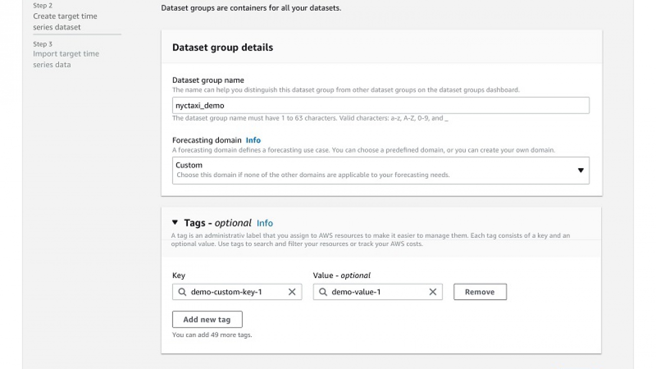
You can add local weather information to your model by adding the Weather Index during training. In this section, we walk through the steps to use the Weather Index on the Forecast console. For this post, we use the New York City Taxi dataset. To review the steps through the APIs, refer to the following notebook in our GitHub repo, where we have a cleaned version of the New York Taxi dataset ready to be used.
The New York Taxi dataset has 260 locations and is being used to predict the demand for taxis per location per hour for the next 7 days (168 hours).
- On the Forecast console, create a dataset group.

- Upload the historical demand dataset as the target time series. This dataset must include geolocation information for you to use the Weather Index.
- Select Schema builder.
- Choose your location format (for this post, the dataset includes latitude and longitude coordinates).
Forecast also supports postal codes for US only.
- For Dataset import details, select Select time zone.
- Choose your time zone (for this post, we choose America/New York).
You can apply a single time zone to the entire dataset, or ask Forecast to derive a time zone from the geolocation of each item ID in the target time series dataset.

- In the navigation pane, under your dataset, choose Predictors.
- Choose Train predictor.

- For Forecast horizon, choose 168.
- For Forecast frequency, choose hour.
- For Number of backtest windows, choose 3.
- For Backtest window offset, choose 168.
- For Forecast types, choose p50, p60, and p70.
- For Algorithm, you can either select AutoML for Forecast to find the best algorithm for your dataset or select a specific algorithm. For this post, we select DeepAR+ with Hyperparameter optimization turned on for Forecast to optimize the model.
- Under Built-in datasets, select Enable Weather Index to apply the Weather Index to your training model. For this post, we have also selected Enable Holidays for US, as we hypothesize that holidays will have an impact on the demand for Taxis.
If you’re following the notebook in our GitHub repo, we call this predictor nyctaxi_demo_weather_deepar. While training the model, Forecast uses the historical weather to apply the Weather Index to only those items that are impacted by weather to improve item level accuracy.

- After your predictor is trained, choose your predictor on the Predictors page to view the details of the accuracy metrics.

- On the predictor’s details page, you can review the model accuracy numbers and choose Export backtest results in the Predictor metrics
Forecast provides different model accuracy metrics for you to assess the strength of your forecasting models. We provide the weighted quantile loss (wQL) metric for each selected distribution point, also called quantiles, and weighted absolute percentage error (WAPE) and root mean square error (RMSE), calculated at the mean forecast. For each metric, a lower value indicates a smaller error and therefore a more accurate model. All these accuracy metrics are non-negative. Quantiles are specified when choosing your forecast type. For more information about how each metric is calculated and recommendations for the best use case for each metric, see Measuring forecast model accuracy to optimize your business objectives with Amazon Forecast.

- For S3 predictor backtest export location, enter the details of your Amazon Simple Storage Service (Amazon S3) location for exporting the CSV files.

Exporting the backtest results downloads the forecasts from the backtesting for each item and the accuracy metrics for each item. This helps you measure the accuracy of forecasts for individual items, allowing you to better understand your forecasting model’s performance for the items that most impact your business. For more information about the benefits of exporting backtest results, see Amazon Forecast now supports accuracy measurements for individual items.
In the next section of this post, we use these backtest results to assess the accuracy improvements of enabling the Weather Index by comparing the accuracy of specific items between models where you have not enabled the Weather Index.
- After you evaluate the model accuracy, you can start creating forecasts by choosing Forecasts in the navigation pane.
- Choose Create a forecast.

To create these forecasts, Forecast automatically pulls in the weather forecasts for the next 14 days and applies the weather prediction to only those item IDs that are influenced by weather. In our example, we create forecasts for the next 7 days with hourly frequency.
Assessing the impact of the Weather Index
To assess the impact of adding weather information to your forecasting models, we can create another predictor with the same dataset and settings, but this time without enabling the Weather Index. If you’re following the notebook in our GitHub repo, we call this predictor nyctaxi_demo_baseline_deepar.
When creating this predictor, you should not select Hyperparameter optimization for DeepAR+, but rather use the winning training parameters from the hyperparameter optimization of DeepAR+ model of nyctaxi_demo_weather_deepar as the training parameters setting, for a fair comparison between the two models. You can find the winning training parameters in the predictor details page under the Predictor metrics section. For this post, these are as follows.
"context_length": "63",
"epochs": "500",
"learning_rate": "0.014138165570842774",
"learning_rate_decay": "0.5",
"likelihood": "student-t",
"max_learning_rate_decays": "0",
"num_averaged_models": "1",
"num_cells": "40",
"num_layers": "2",
"prediction_length": "168"
You can then go to the Predictors page to review the predictor metrics nyctaxi_demo_baseline_deepar.
The following screenshot shows the predictor details page for the nyctaxi_demo_baseline_deepar model that is trained without enabling the Weather Index. The predictor metrics for nyctaxi_demo_weather_deepar with weather enabled is shown above after the create predictor steps.

The following table summarizes the predictor metrics for the two models. Forecast provides the weighted quantile loss (wQL) metric for each quantile, and weighted absolute percentage error (WAPE) metric and root mean square error (RMSE) metric, calculated at the mean forecast. For each metric, a lower value indicates a smaller error and therefore a more accurate model. The model with the Weather Index is more accurate, with lower values for each metric.
| Predictor | wQL[0.5] | wQL[0.6] | wQL[0.7] | WAPE | RMSE |
| nyctaxi_demo_baseline_deepar | 0.2637 | 0.2769 | 0.2679 | 0.2625 | 31.3986 |
| nyctaxi_demo_weather_deepar | 0.1646 | 0.1620 | 0.1498 | 0.1647 | 19.7874 |
You can now export the backtest results for both predictors to assess the forecasting accuracy at an item level. With the backtest results, you can also use a visualization tool like Amazon QuickSight to create graphs that help you visualize and compare the model accuracy of both the predictors by plotting the forecasts against actuals for items that are important for you. The following graph visualizes the comparison of the models with and without the Weather Index to the actual demand for a few items in the dataset at the 0.60 quantile.

For Feb 27, we have zoomed in to better assess the difference in accuracies at an hourly level.

Here we show the magnitude of error for each item id for the two models. Lower error values correspond to a more accurate model. Most items in the model with the Weather Index have errors below 0.05.

Tips and best practices
When using the Weather Index, consider the following best practices:
- Before using the Weather Index, define your use case and the forecasting challenge. Evaluate if your business problem will be impacted by day-to-day weather, because the Weather Index is only available for short-term use cases of 14-day forecasts. Weekly, monthly, and yearly frequencies aren’t supported, so use cases where you are forecasting for the next season don’t benefit from the Weather Index. Only daily, hourly and minute frequencies are acceptable to use the Weather Index.
- For experimentation, start by identifying the most important item IDs for your business that you want to improve your forecasting accuracy. Measure the accuracy of your existing forecasting methodology as a baseline and compare that to the accuracy of those items with Forecast.
- Incrementally add the Weather Index, related time series, or item metadata to train your model to assess whether additional information improves accuracy. Different combinations of related time series, item metadata and built-in datasets can give you different results.
- To assess the impact of the Weather Index, first train a model with only your target time series, and then create another model with the Weather Index enabled. We recommend to use the same predictor settings for this comparison, because different hyperparameters and combinations of related time series can give you different results.
- You may see an increase in training costs when using the Weather Index, because the index is applied and optimized for only those items that are impacted by day-to-day weather variation. However, there is no extra cost to access the weather information or use the Weather Index for creating forecasts. The cost for training continues to be $0.24 per training hour and $0.60 per 1,000 forecasts.
- Experiment with multiple distribution points to optimize your forecast model to balance the costs associated with under-forecasting and over-forecasting. Choose a higher quantile if you want to over-forecast to meet demand.
- If you’re comparing different models, use the weighted quantile loss metric at the same quantile for comparison. The lower the value, the more accurate the forecasting model.
- Forecast allows you to select up to five backtest windows. Forecast uses backtesting to tune predictors and produce accuracy metrics. To perform backtesting, Forecast automatically splits your time series datasets into two sets: training and testing. The training set is used to train your model, and the testing set to evaluate the model’s predictive accuracy. We recommend choosing more than one backtest window to minimize selection bias that may make one window more or less accurate by chance. Assessing the overall model accuracy from multiple backtest windows provides a better measure of the strength of the model.
Conclusion
With the Amazon Forecast Weather Index, you can now automatically include local weather information to your demand forecasts with one click and at no extra cost. The Weather Index combines multiple weather metrics from historical weather events and current forecasts at a given location to increase your demand forecast model accuracy. To get started with this capability, see Weather Index and go through the notebook in our GitHub repo that walks you through how to use the Forecast APIs to enable the Weather Index. You can use this capability in all Regions where Forecast is publicly available. For more information about Region availability, see AWS Regional Services.
About the Authors

Namita Das is a Sr. Product Manager for Amazon Forecast. Her current focus is to democratize machine learning by building no-code/low-code ML services. On the side, she frequently advises startups and is raising a puppy named Imli.
 Gunjan Garg is a Sr. Software Development Engineer in the AWS Vertical AI team. In her current role at Amazon Forecast, she focuses on engineering problems and enjoys building scalable systems that provide the most value to end-users. In her free time, she enjoys playing Sudoku and Minesweeper.

Christy Bergman is working as an AI/ML Specialist Solutions Architect at AWS. Her work involves helping AWS customers be successful using AI/ML services to solve real-world business problems. Prior to joining AWS, Christy worked as a data scientist in banking and software industries. In her spare time, she enjoys hiking and bird watching.
AWS democratizes access to the largest genomic sequences repository — NIH’s Sequence Read Archive
For the first time, the largest genomic sequencing repository in the Americas will be natively accessible on AWS through the Open Data Sponsorship Program.Read More

New Amazon SageMaker Neo features to run more models faster and more efficiently on more hardware platforms
Amazon SageMaker Neo enables developers to train machine learning (ML) models once and optimize them to run on any Amazon SageMaker endpoints in the cloud and supported devices at the edge. Since Neo was first announced at re:Invent 2018, we have been continuously working with the Neo-AI open-source communities and several hardware partners to increase the types of ML models Neo can compile, the types of target hardware Neo can compile for, and to add new inference performance optimization techniques.
As of this writing, Neo optimizes models trained in DarkNet, Gluon, Keras, MXNet, PyTorch, TensorFlow, TensorFlow-Lite, ONNX, and XGBoost for inference on Android, iOS, Linux, and Windows machines based on processors from Ambarella, Apple, ARM, Intel, NVIDIA, NXP, Qualcomm, Texas Instruments, and Xilinx. Models optimized by Neo can perform up to 25 times faster with no loss in accuracy.
Over the past few months, Neo has added a number of key new features:
- Expanded support for PC and mobile devices
- Heterogeneous execution with NVIDIA TensorRT
- Bring Your Own Codegen (BYOC) framework
- Inference optimized containers
- Compilation for dynamic models
In this post, we summarize how these new features allow you to run more models on more hardware platforms both faster and more efficiently.
Expanded support for PC and mobile devices
Earlier in 2020, Neo launched support for Windows on x86 processor-based devices, allowing you to run your models faster and more efficiently on personal computers and other Windows devices. In addition, Neo launched support for Android on ARM-based processors and Qualcomm processors with Hexagon DSP.
Most recently, Apple and AWS partnered to automate model conversion to Core ML format using Neo. As a result, ML app developers can now train models in SageMaker and convert them to Core ML format with a click of button, and deploy the models on iOS and MacOS devices.
Heterogeneous execution with NVIDIA TensorRT
Neo uses the NVIDIA TensorRT acceleration library to increase the speedup of ML models on NVIDIA Jetson devices at the edge and AWS g4dn and p3 instances in the AWS Cloud. The TensorRT library supports a subset of operators commonly used in deep learning models.
Previously, Neo used TensorRT only when the entire computational graph of the model and all its operators could be accelerated by the library. As a result, few models could take advantage of TensorRT acceleration.
Recently, Neo added the capability to partition a model into sub-graphs, in which case a part of the model can be handled by TRT while the other part can be compiled by Apache TVM. To execute the compiled model, Neo runtime uses the heterogeneous execution mechanism to run both parts on the hardware. With this approach, Neo can provide the best available performance for a broader range of frameworks and models.
Bring your own codegen
We also expanded the heterogeneous execution approach to other hardware targets. Neo partnered with chip vendors to use the Bring Your Own Codegen (BYOC) mechanism in TVM to plug in partners’ proprietary toolchains for their ML accelerators, such as Ambarella’s CV Tools and Texas Instruments’ TIDL, with the Neo compilation API.
When you compile, Neo partitions a model so you can run the supported portion supported in the ML accelerators and the rest on the host CPU. With this approach, Neo maximizes the utilization of the ML accelerator on the chip, increases the types of models that you can compile for the chip, and makes it easier for you to take advantage of new ML accelerators from chip vendors.
Inference optimized containers
Like all deep learning compilers, Neo supports a subset of operators and models in a given framework. Before adding this feature, Neo could only compile a model if all the operators from the model were supported by Neo. Now, when you use Neo to compile a MXNet, PyTorch, or TensorFlow model for CPU or GPU inferences in SageMaker hosted endpoints on AWS, Neo partitions the models, compiles a portion to accelerate performance, and leaves the un-compiled part of the model to continue running natively in the framework. You can use Neo’s inference optimized containers to deploy on SageMaker hosted endpoints. As a result, you can optimize any MXNet, PyTorch, and TensorFlow model with Neo for any SageMaker hosted endpoint.
Compilation for dynamic models
Deep learning models contain dynamic features, such as control flow, dynamic operations, dynamic data structures, and dynamic input and output shapes that pose significant challenges to existing deep learning compilers. These models, including some object detection and semantic segmentation models, are becoming increasingly popular. Recently, we added the ability in Neo to compile these dynamic models. You can now use Neo to optimize models with dynamic features, and get up to two times the performance speedup.
Summary
We continually make improvements and add supported hardware endpoints, models, and frameworks to Neo based on your feedback. We encourage you to sign in to the SageMaker console or use the Neo compilation API to compile your trained models for the target hardware of your interest. For more information about Neo, see the following:
- Speeding up TensorFlow, MXNet, and PyTorch inference with Amazon SageMaker Neo
- Optimizing ML models for iOS and MacOS devices with Amazon SageMaker Neo and Core ML
- Amazon SageMaker Neo makes it easier to get faster inference for more ML models with NVIDIA TensorRT
- Model dynamism Support in Amazon SageMaker Neo
About the Authors
 Tingwei Huang is a product management leader at AWS AI Service.
 Vin Sharma is a Engineering Leader for AWS Deep Learning. He leads the team building Neo, which helps ML models train once and run anywhere in the cloud and at the edge.

Model dynamism Support in Amazon SageMaker Neo
Amazon SageMaker Neo was launched at AWS re:Invent 2018. It made notable performance improvement on models with statically known input and output data shapes, typically image classification models. These models are usually composed of a stack of blocks that contain compute-intensive operators, such as convolution and matrix multiplication. Neo applies a series of optimizations to boost the model’s performance and reduce memory usage. The static feature significantly simplifies the compilation, and you can decide on runtime inference tasks such as memory sizes ahead of time using a dedicated analysis pass. Runtime is just acted as a topological graph walker that invokes each operator sequentially.
However, we have been seeing a growing number of customers requiring more advanced models to fulfill tasks like object detection. These models contain dynamic features, such as control flow, dynamic operations, dynamic data structures, and dynamic input and output shapes. This posts significant challenges to the existing deep learning compiler because they have been mainly confined to static models. To address this problem, existing solutions either use just-in-time compilation to compile and run the dynamic portion (XLA), which causes extra compilation overhead, or convert the dynamic model into a static representation first (TFLite). To meet your requirements, we designed and implemented a suite of techniques ranging from the front-end parser to the backend runtime to handle object detection and segmentation models trained by TensorFlow, PyTorch, and MXNet. In this post, we’ll walk you through how Neo supports object detection and semantic segmentation models. We also compare inference performance improvements for both instance and edge type devices for Neo object detection and segmentation models.
Methodology
This section describes how object detection and semantic segmentation models are supported in Neo. We discuss the following:
- How the front end handles popular frameworks differently
- How the backend is designed to support dynamism
- An example using the AWS Command Line Interface (AWS CLI) to demonstrate how to easy it is to perform inference for an object detection model in Neo
Frontend
The approaches vary for each framework because they handle dynamism, particularly control flow, differently. For example, MXNet doesn’t use any control flow to implement the object detection and segmentation models, which allows us to have a quick one-to-one operator mapping from MXNet to Relay operators. PyTorch has control flow primitives, such as If and Loop, which largely simplifies the conversion because we can create Relay If statements and recursion functions correspondingly.
Among the most popular frameworks, TensorFlow is the most difficult to support because it doesn’t directly employ conditional and looping operators to implement control flow. Instead, low-level data flow primitives, such as Merge, Exit, Switch, NextIteration, and Enter, are used to express complex control flow logic for the better support of parallel and distributed execution. For more information, see Implementation of Control Flow in TensorFlow.
To decompile these primitives into the original control flow operators, we proposed dedicated analysis and pattern matching techniques that have been contributed back to the Apache TVM. For more information, see the RFC Decompile TensorFlow Control Flow Primitives to Relay and Enhance TensorFlow Frontend Control Flow Support.
Backend
The backend compiler has worked well in supporting static models where the input data type and shape for each tensor is known at the compile-time. However, this assumption doesn’t hold for dynamic models, such as TensorFlow SSD, because the data shapes can only be determined at runtime.
To support dynamic data shapes, we introduced a special dimension called Any to represent statically unknown dimensions. For instance, a tensor type could be represented as Tensor[(5, Any), float32], where the second dimension was unknown. Accordingly, we defined some type inference rules to infer the type of the tensor when Any shape is involved.
To get the data shape of a tensor at runtime, we defined shape functions to compute the output shape of the tensor to determine the size of required memory. Based on the categories of the operators, shape functions were classified into three patterns:
- Data-independent shapes – Are used for operators whose output shape is only determined by the shapes of the inputs, such as 2D convolution.
- Data-dependent shapes – Require the real input value instead of the shape to compute the output shapes. For example,
arangeneeds the value ofstart,stop, andstepto compute the output shape. - Upper bound shapes – Are used to quickly estimate an upper bound shape for the output in order to avoid redundant computation. This is useful because operators, such as Non Maximum Suppression (NMS), involve non-trivial computation to infer the output shape at runtime, and the amount of computation for the shape function could be on par with that of running the operator.
To effectively run the dynamic models, we designed a virtual machine as an execution engine to invoke runtime type inference, handle control flow, and dispatch operator kernels. We compiled the model into a machine-dependent kernel code and machine-independent bytecode. They were then loaded and run by the virtual machine.
Because each instruction works on coarse-grained data, such as tensor, the instructions are compactly organized, meaning the dispatching overhead isn’t a concern. We designed the virtual machine in a register-based manner to simplify the design and allow users to read and modify the code easily. We designed a set of instructions to control running each type of bytecode, such as storage allocation, tensor memory allocation on the storage, control flow, and kernel invocation.
After the virtual machine loads the compiled bytecode and kernels, it interprets the bytecode in a dispatching loop by checking it op-code and invoking appropriate logic. For more information, see Nimble: Efficiently Compiling Dynamic Neural Networks for Model Inference.
Performing inference and object detection in Neo
This section provides an example to illustrate how you can compile a Faster R-CNN model from TensorFlow 1.15 and deploy it on an AWS C5 instance using Neo.
- Prepare the pre-trained model by downloading it from the TensorFlow Detection Model Zoo and extracting it:
$ wget http://download.tensorflow.org/models/object_detection/faster_rcnn_resnet50_coco_2018_01_28.tar.gz
$ tar -xzf faster_rcnn_resnet50_coco_2018_01_28.tar.gz
- Get the frozen protobuf file and upload it to Amazon Simple Storage Service (Amazon S3):
$ tar -czf tf_frcnn.tar.gz faster_rcnn_resnet50_coco_2018_01_28.tar.gz
$ aws s3 cp tf_frcnn.tar.gz s3://<your-bucket>/<your-input-folder>
We can now compile the model using Neo. For this post, we use the AWS CLI. We first create a configuration JSON file where the required information is fed (such as the input size, framework, location of the output artifacts, and target platform that we compile the model for):
- Create the configuration file with the following code:
{
    "CompilationJobName": "compile-tf-ssd",
    "RoleArn": "arn:aws:iam::<your-account>:role/service-role/AmazonSageMaker-ExecutionRole-yyyymmddThhmmss",
    "InputConfig": {
        "S3Uri": "s3://<your-bucket>/<your-input-folder>/tf_frcnn.tar.gz",
        "DataInputConfig":  "{'image_tensor': [1,512,512,3]}",
        "Framework": "TENSORFLOW"
    },
    "OutputConfig": {
        "S3OutputLocation": "s3://<your-bucket>/<your-output-folder>",
        "TargetPlatform": {
            "Os": "LINUX",
            "Arch": "X86_64"
        },
        "CompilerOptions": "{'mcpu': 'skylake-avx512'}"
    },
    "StoppingCondition": {"MaxRuntimeInSeconds": 1800}
}
- Compile it with SageMaker CLI:
$ aws sagemaker create-compilation-job --cli-input-json file://config.json --region us-west-2
Finally, we’re ready to deploy the compiled model with DLR.
- Before the deployment, download the compiled artifacts from the S3 bucket where it was saved to:
$ aws s3 cp s3://<your-bucket>/<output-folder>/output_artifacts.tar.gz tf_frcnn_compiled.tar.gz
$ mkdir compiled_model
$ tar -xzf tf_frcnn_compiled.tar.gz -C compiled_model
- Install DLR for inference:
$ pip install dlr
- Perform inference as the following:
if __name__ == "__main__":
    data = cv2.imread("input_image.jpg")
    data = cv2.resize(data, (512, 512), interpolation=cv2.INTER_AREA)
    data = np.expand_dims(data, 0)
    model = dlr.DLRModel('compiled_model', 'cpu', 0)
    result = model.run(data)
Performance comparison
In this section, we compare the performance of the most widely used TF object detection and segmentation models on a variety of EC2 server platforms and NVIDIA Jetson based edge devices. We use the models from the TensorFlow Detection Model Zoo. As discussed earlier, these models show dynamism and are significantly more complex than the static models like ResNet50. We use Neo to compile these models and generate high-performance machine code for a variety of target platforms. Here, we show the performance comparison for these models across many hardware devices against the best baseline available for the hardware platforms.
EC2 C5.9x large server instance
C5 instances are Intel Xeon server instances suitable for compute-intensive deep learning applications. For this comparison, we report the average latency for the TensorFlow baseline and Neo-compiled model. All the reported latency numbers are in milliseconds. We observe that Neo outperforms TensorFlow for all the three models, and by up to 20% for the Mask R-CNN ResNet-50 model.
| Model name | TF 1.15.0 | Neo | Speedup |
| ssd_mobilenet_v1_coco | 17.96 | 16.39 | 1.09579 |
| faster_rcnn_resnet50_coco | 152.62 | 142.3 | 1.07252 |
| mask_rcnn_resnet50_atrous_coco | 391.91 | 326.44 | 1.20056 |
EC2 m6g.8x large server instance
M6 instances are the ARM Graviton server instances suitable for compute-intensive deep learning applications. To get a baseline, we use the TensorFlow packages provided from ARM Tool-Solutions. Our observations are similar to C5 instances. Neo outperforms TensorFlow, and we observe significant speedup for large models like Faster RCNN and MaskRCNN.
| Model name | TF 1.15.0 | Neo | Speedup |
| ssd_mobilenet_v1_coco | 29.04 | 28.75 | 1.01009 |
| faster_rcnn_resnet50_coco | 290.64 | 202.71 | 1.43377 |
| mask_rcnn_resnet50_atrous_coco | 623.98 | 368.81 | 1.69187 |
NVIDIA server instance and edge devices
Finally, we compare the performance of the MobileNet SSD model on NVIDIA Jetson based edge devices—Jetson Xavier and Jetson Nano. MobileNet SSD is a popular object detection model for edge devices. This is because it has low compute and memory requirements, and is suitable for already resource-constrained edge devices. To have a performance baseline, we use the TF-TRT package, where TensorFlow is integrated with NVIDIA TensorRT as the backend. We present the comparison in the following table. We observe that Neo achieves significant speedup for both Xavier and Nano edge devices.
| Performance comparison for ssd_mobilenet_v1_coco | |||
| Hardware device | TF 1.15 | Neo | Speedpup |
| NVIDIA Jetson Nano | 163 | 140 | 1.16429 |
| Jetson Xavier | 109 | 56 | 1.94643 |
Summary
This post described how Neo supports model dynamism. Multiple techniques were proposed from the front-end parser to backend runtime to enable the model support. We compared the inference performance of Neo object detection and segmentation models against those required by the TensorFlow framework or TensorFlow backed with TensorRT. We observed that Neo obtained speedups for these models on both instances and edge devices.r
This solution doesn’t have any the service API changes, so you can still use the original API to compile new models. All code has been contributed back to the Apache TVM. For more information about compiling a model using Apache TVM, see Compile PyTorch Object Detection Models.
Acknowledgements: We sincerely thank the following engineers and applied scientists who have contributed to the support of dynamic models: Haichen Shen, Wei Chen, Yong Wu, Yao Wang, Animesh Jain, Trevor Morris, Rohan Mukherjee, Ricky Das
About the Author

Zhi Chen is a Senior Software Engineer at AWS AI who leads the deep learning compiler development in Amazon SageMaker Neo. He helps customers deploy the pre-trained deep learning models from different frameworks on various platforms. Zhi obtained his PhD from University of California, Irvine in Computer Science, where he focused on compilers and performance optimization.

Amazon SageMaker Neo makes it easier to get faster inference for more ML models with NVIDIA TensorRT
Amazon SageMaker Neo now uses the NVIDIA TensorRT acceleration library to increase the speedup of machine learning (ML) models on NVIDIA Jetson devices at the edge and AWS g4dn and p3 instances in the AWS Cloud. Neo compiles models from TensorFlow, TFLite, MXNet, PyTorch, ONNX, and DarkNet to make optimal use of NVIDIA GPUs, providing you with the best available performance from the hardware for a broader range of frameworks and models, without the need to learn the nitty-gritty details of deep learning frameworks and acceleration libraries.
The NVIDIA TensorRT library supports a subset of operators commonly used in deep learning models. Previously, Neo used TensorRT only when the entire computational graph of the model and all its operators could be accelerated by the library. As a result, the use of the library was limited mostly to image classification models.
Now, Neo takes advantage of TensorRT for all models, even when a model contains operators that the library doesn’t support. Neo does this by partitioning the model into sub-graphs, in which TRT handles one type of sub-graph and Apache TVM handles the other. Then, at runtime, Neo uses a new heterogeneous execution mechanism to run both types of sub-graphs with the same runtime.
With this approach, Neo automatically takes advantage of TensorRT to accelerate computation-heavy operations, such as convolutions supported by the accelerator library, while generating highly performant CUDA code for all other operations using Apache TVM. As a result, Neo delivers better performance for more models than either NVIDIA TRT or Apache TVM alone.
The Neo team generalized this approach into a mechanism we call Bring Your Own Codegen. It allows us to easily extend this work to new hardware partners, who can bring their own accelerator libraries to take advantage of the wide range of frameworks and models covered by Neo while improving performance to the full extent possible on their hardware.
Performance highlights
The following table summarizes the platform, corresponding framework, model, and latency performance.
| Platform | Framework | Model | Latency |
| Jetson Xavier | TensorFlow | SSD MobilenetV2 COCO |
49.71ms
|
| MXNet | SSD MobileNet 1.0 VOC | 19.7ms | |
| Pytorch | YoloV4 | 68.76ms | |
| DarkNet | YoloV3 Tiny | 18.98ms | |
| Jetson Nano | TensorFlow | SSD MobilenetV2 COCO | 223.69ms |
| MXNet | SSD MobileNet 1.0 VOC | 131.58ms | |
| DarkNet | YoloV3 Tiny | 41.73ms |
Conclusion
We’re very excited to offer this new integration with TensorRT, which allows you to speed up inference for your ML models. To get started with Amazon SageMaker Neo for NVIDIA Jetson or AWS g4dn, p3, and p2 instances, see Amazon SageMaker Neo.
About the Author
 Trevor Morris is a Software Engineer at AWS AI working on compiler technology and optimization for machine learning inference. He focuses on improving performance for GPUs, with previous experience at NVIDIA.
Optimizing ML models for iOS and MacOS devices with Amazon SageMaker Neo and Core ML
Core ML is a machine learning (ML) model format created and supported by Apple that compiles, deploys, and runs on Apple devices. Developers who train their models in popular frameworks such as TensorFlow and PyTorch convert models to Core ML format to deploy them on Apple devices.
Recently, Apple and AWS partnered to automate model conversion to Core ML in the cloud using Amazon SageMaker Neo. Neo is an ML model compilation service on AWS that enables you to automatically convert models trained in TensorFlow, PyTorch, MXNet, and other popular frameworks, and optimize them for the target of your choice. With the new automated model conversion to Core ML, Neo now makes it easier to build apps on Apple’s platform to convert models from popular libraries like TensorFlow and PyTorch to Core ML format.
In this post, we show how to set up automatic model conversion, add a model to your app, and deploy and test your new model.
Prerequisites
To get started, you first need to create an AWS account and create an AWS Identity and Access Management (IAM) administrator user and group. For instructions, see Set Up Amazon SageMaker. You will also need Xcode 12 installed on your machine.
Converting models automatically
One of the biggest benefits of using Neo is automating model conversion from a framework format such as TensorFlow or PyTorch to Core ML format by hosting the coremltools library in the cloud. You can do this via the AWS Command Line Interface (AWS CLI), Amazon SageMaker console, or SDK. For more information, see Use Neo to Compile a Model.
You can train your models in SageMaker and convert them to Core ML format with the click of a button. To set up your notebook instance, generate a Core ML model, and create your compilation job on the SageMaker console, complete the following steps:
- On the SageMaker console, under Notebook, choose Notebook instances.

- Choose Create notebook instance.
- For Notebook instance name, enter a name for your notebook.
- For Notebook instance type¸ choose your instance (for this post, the default ml.t2.medium should be enough.
- For IAM role, choose your role or let AWS create a role for you.
After the notebook instance is created, the status changes to InService.
- Open the instance or JupyterLab.
You’re ready to start with your first Core ML model.
- Begin your notebook by importing some libraries:
import warnings
 warnings.simplefilter(action='ignore', category=FutureWarning)

 import sagemaker
 from PIL import Image
 import torch
 import torch.nn as nn
 import torchvision
 from torchvision import transforms
- Choose the following image (right-click) and save it.
You use this image for testing the model later, and it helps make the segmentation model.

- Upload this image in your local directory. If you’re using a SageMaker notebook instance, you can upload the image by choosing Upload.

- To use this image, you need to format it so that it works with the segmentation model when testing the model’s output. See the following code:
# Download the sample image. For this I right-clicked and copied and pasted what
 # was on the website and used it locally.
 input_image = Image.open("dog_and_cat.jpg")

 preprocess = transforms.Compose([
     transforms.ToTensor(),
     transforms.Normalize(
         mean=[0.485, 0.456, 0.406],
         std=[0.229, 0.224, 0.225],
     ),
 ])
 input_tensor = preprocess(input_image)
 input_batch = input_tensor.unsqueeze(0)
You now need a model to work with. For this post, we use the TorchVision deeplabv3 segmentation model, which is publicly available.
The deeplabv3 model returns a dictionary, but we want only a specific tensor for our output.
- To remedy this, wrap the model in a module that extracts the output we want:
class WrappedDeeplabv3Resnet101(nn.Module):

    def __init__(self):
        super(WrappedDeeplabv3Resnet101, self).__init__()
        self.model = torch.hub.load(
            'pytorch/vision:v0.6.0',
            'deeplabv3_resnet101',
            pretrained=True
        ).eval()

    def forward(self, x):
        res = self.model(x)
        # Extract the tensor we want from the output dictionary
        x = res["out"]
        return x
- Trace the PyTorch model using a sample input:
traceable_model = WrappedDeeplabv3Resnet101().eval()
 trace = torch.jit.trace(traceable_model, input_batch)
Your model is now ready.
- Save your model. The following code saves it with the .pth file extension:
trace.save('DeepLabV3.pth')Your model artifacts must be in a compressed tarball file format (.tar.gz) for Neo.
- Convert your model with the following code:
import tarfile
 with tarfile.open('DeepLabV3.tar.gz', 'w:gz') as f:
     f.add('DeepLabV3.pth')
- Upload the model to your Amazon Simple Storage Service (Amazon S3) bucket.
If you don’t have an S3 bucket, you can let SageMaker make one for you by creating a sagemaker.Session(). The bucket has the following format: sagemaker-{region}-{aws-account-id}. Your model must be saved in an S3 bucket in order for Neo to access it. See the following code:
import sagemaker
 sess = sagemaker.Session()
 bucket = sess.default_bucket()
- Specify the directory where you want to store the model:
prefix = 'model' # Output directory in your S3 bucket- Upload the model to Amazon S3 and print out the S3 bucket path URI for future reference:
model_path = sess.upload_data(path='DeepLabV3.tar.gz', key_prefix=prefix)
 print(model_path)
- On the SageMaker console, under Inference, choose Compilation jobs.

- Choose Create compilation job.
- In the Job settings section, for Job name, enter a name for your job.
- For IAM role, choose a role.

- In the Input configuration section, for Location of model artifacts, enter the location of your model. Use the path from the print statement earlier (
print(model_path)). - For Data input configuration, enter the shape of the model tensor. For this post, the TorchVision
deeplabv3segmentation model has the shape[1,3,448,448]. - For Machine learning framework, choose PyTorch.

- In the Output configuration section, select Target device.
- For Target device, choose coreml.
- For S3 Output location, enter the output location of the compilation job (for this post,
/output). - Choose Submit.

You’re redirected to the Compilation jobs page on the SageMaker console. When the compilation job is complete, you see the status COMPLETED.
If you go to your S3 bucket, you can see the output of the compilation job. The output has an .mlmodel file extension.

The output of the Neo service CreateCompilationJob is a model in Core ML format, which you can download from the S3 bucket location to your Mac. You can use this conversion process with any type of model that coremltools supports—from image classification or segmentation, to object detection or question answering text recognition.
Adding the model to your app
Make sure that you have installed Xcode version 12.0 or later. For more information about using Xcode, see the Xcode documentation. To add the converted Core ML model to your app in Xcode, complete the following steps:
- Download the model from the S3 bucket location.
- Drag the model to the Project Navigator in your Xcode app.

- Select any preferred options.
- Choose Finish.

- Choose the model in the Xcode Project Navigator to see its details, including metadata, predictions, and utilities.

- Choose the Predictions tab to see the model’s input and output.

Deploying and testing the model
Xcode automatically generates a Swift model class for the Core ML model, which you can use in your code to pass inputs.

For example, to load the model in your code, use the following model class:
let model = DeepLabV3()You can now pass through input values using the model class. To test that your app is performing as expected with the model, launch the app in the Xcode simulator and target a specific device. If it works in the Xcode simulator, it works on the device!
Conclusion
Neo has created an easy way to generate Core ML format models from TensorFlow and PyTorch. You’re not required to learn about the coremltools library or how to convert their models in TensorFlow or PyTorch to Core ML format. After you convert your model to Core ML format, you can follow a well-defined path to compile and deploy your model to an iOS device or Mac computer. If you’re already a SageMaker customer, you can train your model in SageMaker and convert it to Core ML format using Neo with the click of a button.
For more information, see the following resources:
- Amazon SageMaker Neo
- Use Neo to Compile a Model
- Set Up Amazon SageMaker
- DeepLabv3-Resnet 101 model
- Converting a PyTorch Segmentation Model to Core ML
- Core ML developer documentation
- Coremltools documentation
- Xcode documentation
- Integrating a Core ML Model into Your App
- coremltools GitHub repo
About the Author
 Lokesh Gupta is a Software Development Manager at AWS AI service.
Speeding up TensorFlow, MXNet, and PyTorch inference with Amazon SageMaker Neo
Various machine learning (ML) optimizations are possible at every stage of the flow during or after training. Model compiling is one optimization that creates a more efficient implementation of a trained model. In 2018, we launched Amazon SageMaker Neo to compile machine learning models for many frameworks and many platforms. We created the ML compiler service so that you don’t need to set up compiler software, such as TVM, XLA, Glow, TensorRT, or OpenVINO, or be concerned with tuning the compiler for best model performance.
Since then, we have updated Neo to support more operators and expand model coverage for TensorFlow, PyTorch, and Apache MXNet (incubating). In October 2020, we made an internal change to allow a model to be partially compiled for CPU and GPU targets. Prior to this change, Neo could only compile a model if all the operators from the model could be compiled. With this change, Neo can figure out which part of the model can be compiled, and generates a model artifact combining the compiled and non-compiled parts. The combined model artifact can be used by SageMaker managed inference endpoints. The non-compiled parts of the model continue running in the framework, while the compiled parts run natively on CPU or GPU. As a result, many more models can see increased inference speeds in SageMaker when they are compiled with Neo.
The interface to model compiling has remained unchanged. This post shows the resulting model performance improvements and the mechanics behind how they work. For a step-by-step tutorial on using Neo to compile a model and deploy in SageMaker managed endpoints, see these notebook examples: Tensorflow mnist, PyTorch VGG19, and MxNet SSD Mobilenet.
Partially compiling a model
In the following example, I took a pre-trained alpha pose model alpha_pose_resnet101_v1b_coco from the GluonCV model zoo and compiled it with Neo. I saved the model from the model zoo into the following two files:
alpha_pose_resnet101_v1b_coco-0000.params
alpha_pose_resnet101_v1b_coco-symbol.json
Then I packed these files into a tar.gz file in an Amazon Simple Storage Service (Amazon S3) bucket and used Neo to compile the model.
Neo compiled the model and created a tar.gz file in an S3 bucket. After downloading and unpacking, I have two files that represent the compiled model (in addition to some other files, which I don’t discuss in detail):
compiled-0000.params
compiled-symbol.json
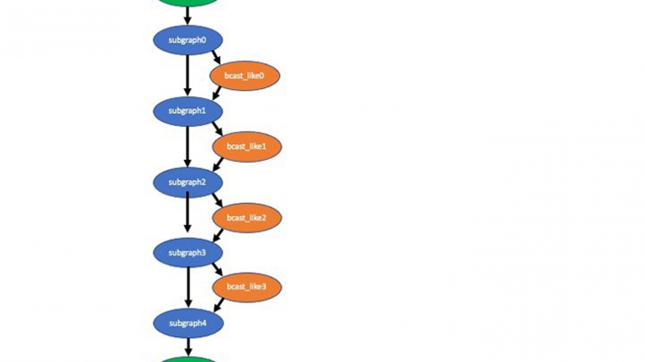
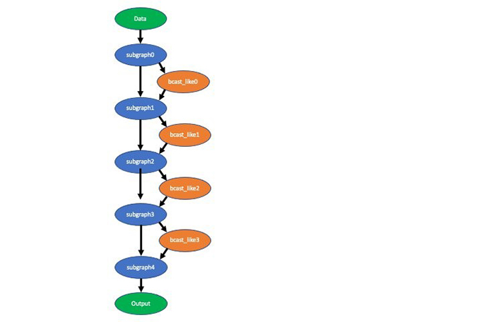
The compiled-symbol.json file contains all nodes of the model graph and edges between nodes. In this case, the Neo compiler service created five optimized subgraphs in the alpha pose model. Each subgraph is represented by the _tvm_subgraph_op node in the model graph. I can use a simple grep command to discover number of subgraphs:
$ cat compiled-symbol.json |grep _tvm_subgraph_op
      "op": "_tvm_subgraph_op",
      "op": "_tvm_subgraph_op",
      "op": "_tvm_subgraph_op",
      "op": "_tvm_subgraph_op",
      "op": "_tvm_subgraph_op",
Next I use a slightly more complex grep command to show you how many ops of each kind are in this model, which ops are in the subgraphs, and which ops are not. The following code block contains 11 instances of the Activation op in all the subgraphs (line is indented), four instances of the broadcast_like op not in any subgraph (line is not indented), and five instances of the subgraph_op:
$ cat compiled-symbol.json | grep ""op"" | grep -v null | sort | uniq -c

     11               "op": "Activation",
    106               "op": "BatchNorm",
    107               "op": "Convolution",
      8               "op": "FullyConnected",
      1               "op": "Pooling",
      9               "op": "Reshape",
      4               "op": "_contrib_AdaptiveAvgPooling2D",
     33               "op": "elemwise_add",
      4               "op": "elemwise_mul",
      8               "op": "expand_dims",
     99               "op": "relu",
      3               "op": "transpose",
      5       "op": "_tvm_subgraph_op",
      4       "op": "broadcast_like",
In a future update of Neo, we may add support to compile the broadcast_like op, in which case the model is entirely compiled.
You can visualize the compiled model with the graph visualization tool. The following visualization depicts the partially compiled alpha pose model. This shows you the data flow between the subgraphs and ops not compiled (broadcast_like).
Even though I’m showing you an example of the Neo compiled artifacts from the GluonCV model zoo, the same subgraph concept applies to the TensorFlow and PyTorch compiled artifacts as well. The format of compiled artifacts is different in these other frameworks.
The following table shows the measured latency speedup of this partially compiled model compared with a non-compiled model on one CPU and one GPU Amazon Elastic Compute Cloud (Amazon EC2) instance. The speedup is specific to the model and instance type because the performance gain achieved varies with model architecture and platform.
| Instance | Speedup |
| c5.9xl | 1.28 |
| g4dn.xl | 1.23 |
Next I deployed the compiled model to SageMaker endpoints using the SageMaker inference container, which is integrated with TVM runtime.
Speedup numbers across common models and frameworks
The following table lists latency speedup that you might see from a few common models in all three frameworks in CPU and GPU instances.
| Framework | Model | Instance | Speedup |
| TensorFlow | resnet50 | c5.9xl | 2.86 |
| TensorFlow | resnet50 | g4dn.xl | 1.86 |
| PyTorch | inception v3 | c5.4xl | 3.03 |
| PyTorch | inception v3 | p3.2xl | 3.53 |
| MXNet | yolo3 | m5.12xl | 1.26 |
| MXNet | yolo3 | g4dn.xl | 1.11 |
These numbers are only general guidelines, as opposed to performance expectations for your specific model and instance choice. The numbers in the table are measured at the instance level and don’t include time spent on preprocessing and postprocessing. In SageMaker hosting, preprocessing and postprocessing can also take time, and is worth looking into in your overall optimization strategy.
How compiling works
In all frameworks (PyTorch, TensorFlow, and MXNet), we start by analyzing the model. We look at clusters of operators that are compilable, and fuse these into subgraphs. We avoid creating too many subgraphs using heuristics. Running subgraphs has an extra cost of data copy and launch overhead. If all operators are compilable in a model, the entire model is a single subgraph with all the operators.
In all frameworks, we use TVM to compile the subgraphs. On Nvidia GPU instance types (g4, p3, p2), we use the TensorRT integration feature of TVM to further identify operators in the subgraphs that can be compiled by TensorRT, creating subgraphs within a subgraph. A hybrid model running on these GPU instances may use the framework runtime, TVM runtime, and TensorRT runtime.
In some dynamic model cases, we use the relayVM from TVM, which has native support for dynamic tensor shape and control flow operators. This allows fully ahead-of-time compilation for models such as Mask R-CNN. As of this writing, compilers such as XLA or TensorRT use just-in-time to handle dynamic tensor shapes, which incur extra compiling cost whenever a new tensor shape is present when running a model.
At the subgraph level, TVM uses a framework-specific front-end component to convert the subgraph into relay IR (intermediate language). Relay IR is very expressive and can support data types, variables, control flow, function calls, and highly parallelizable compute operations such as matrix multiplication.
From relay IR, TVM does two types of optimizations: graph level and node or tensor level. One kind of graph-level optimization is to fuse two or more nodes together to avoid extra data copy. This is especially useful when GPU is involved because launching a small kernel too many times is very expensive. Another kind of graph-level optimization is to change the way a multi-dimensional array is stored in memory based on the operators involved. An example is that the conv2D operator used in computer vision models prefers the 4-D array sent to it to be in the NCHW format. Yet another optimization is to pre-compute parts of the subgraph at compile time (constant folding). By rewriting the graph in certain ways, TVM can improve the run speed of the model.
Node- or tensor-level optimization is about generating more efficient code for the operator. For example, the most optimal way of doing conv2D depends on the size of the 4-D array in each dimension. TVM can take advantage of this knowledge and generate code based on the hardware attributes of the target device, such as L1 cache size and CPU or GPU instruction scheduling policies.
Summary
Neo can now compile nearly all ML models from TensorFlow, PyTorch, and MXNet frameworks for SageMaker CPU and GPU instances. We continue to tune and optimize Neo. If you have any questions or comments, use the Amazon SageMaker Discussion Forums or send an email to amazon-neo-feedback@amazon.com.
About the Author
 Wei Xiao is a Principle Engineer working on the optimization of machine learning systems in the Amazon AWS AI org. Previously he worked on distributed systems and relational databases in Amazon and Microsoft for many years.
Predicting soccer goals in near real time using computer vision
In a soccer game, fans get excited seeing a player sprint down the sideline during a counterattack or when a team is controlling the ball in the 18-yard box because those actions could lead to goals. However, it is difficult for human eyes to fully capture such fast movements, let alone predict goals. With machine learning (ML), we can incorporate more fine-grained information at the pixel level to develop a solution that predicts goals with high confidence before they happen.
Sportradar, a leading real-time sports data provider that collects and analyzes sports data, and the Amazon ML Solutions Lab collaborated to develop a computer vision-based Soccer Goal Predictor to detect exciting moments that lead to goals, thereby increasing fan engagement and helping broadcasters provide viewers an enhanced experience. Most action recognition models are used to identify events when they occur, but Amazon ML Solutions Lab developed a novel computer vision-based Soccer Goal Predictor that can predict future soccer goals 2 seconds in advance of the event.
“We deliberately threw one of the hardest possible computer vision problems at the Amazon ML Solutions Lab team to see what the art of the possible could do, and I am very impressed with the results,” says Ben Burdsall, Group CTO at Sportradar. “The team built a video action recognition model to predict future soccer goals two seconds in advance using Amazon SageMaker and demonstrated its application for match intensity tracking. This has opened doors to many new business opportunities. The implementation costs and latency of this model on our production pipeline using AWS’s infrastructure also look very encouraging. After today, I have no more skepticism about the potential of computer vision in innovating our business.”
The team used Amazon SageMaker notebook instances to create a data processing pipeline that extracted training examples from raw videos and used transfer learning to fine-tune an Inflated 3D Networks (I3D) model. The results have inspired Sportradar’s data science and innovation teams to develop new statistics to embed into their broadcast videos to enhance fan engagement.
This post explains how we applied transfer learning using an I3D model towards goal prediction and used the inference to create an intensity index to quantify the likelihood of a team scoring goals. Additionally, we discuss how we constructed a momentum index to measure the change of velocity during attacks. (Attack is a soccer term used to describe the movement of the team in possession of the ball.) With the intensity index and the momentum index, we can detect whether there is an intense moment (a moment that leads to a goal) in near-real-time using live feeds, and build products to help broadcasters engage fans during broadcasts.
Processing the data and building the model
To capture these intense moments, we translated this objective into a binary classification problem: differentiating activities that lead to goals from those that do not. The samples in the positive class (goals class) are video clips that are 2 seconds away from the goals, and the ones from the negative class are clips in which players are engaged in activities that do not lead to goals (ballsafe class). We generated 1,550 clips from 398 professional soccer matches provided by Sportradar.
A lot of action can happen in a few seconds during soccer matches, so we used short video clips to train the model. For this use case, we extracted 5-second clips. A challenge with video processing is that reading multiple video streams and extracting clips sequentially can be very time-consuming, taking several hours to complete. To speed up the clip-extraction process, we created a data pipeline using multiprocessing in an Amazon SageMaker notebook using ml.c5.18xlarge instance with 72 CPUs to parallelize the I/O-heavy clip extraction process and reduced the clip-extraction time from 12 hours to under 15 minutes.
After data processing, we built a binary classification model using the I3D model from GluonCV’s model zoo. The I3D model uses 3D convolutions to learn spatiotemporal information directly from videos. Given that we did not have a large dataset, we employed transfer learning and fine-tuned the I3D model to get well-performant video models with our own data. For more information about fine-tuning and an I3D model using GluonCV, see Fine-tuning SOTA video models on your own dataset.
Using Amazon SageMaker notebook instances, we first loaded an I3D network pre-trained on the Kinetcis400 dataset into a Jupyter notebook. We then fine-tuned this network on the data from Sportradar to find the best set of parameters, especially those specific to action recognition models (e.g., number of frames, number of segments, stride for frame sampling).
Results
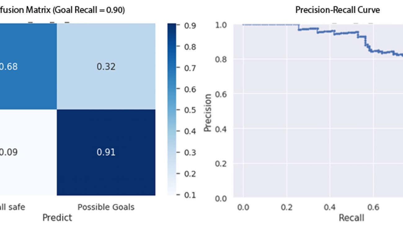
We used recall as our primary metric for model evaluation because we wanted to capture near-100% goals (positive class). The following graphs depict the confusion matrix and the precision-recall curve. It can be seen that it is difficult for the model to differentiate between the two classes when we have near-100% recall. We re-calibrated the predicted probabilities to look at the model performance for achieving 80% and 90% recall for the positive class (sequence leads to a goal) respectively.
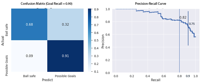
The following table shows the precision and recall of the negative class when we fix the recall of the positive class. We can see that our model can differentiate the two classes with the new settings. When we fix the recall of the positive class at 90%, we can capture 68% of the negative class samples, and the precision is 75%.
| At 80% Goal Recall | At 90% Goal Recall | |
| Ballsafe Recall | 0.81 | 0.68 |
| Goal Precision | 0.82 | 0.75 |
Intensity index and momentum index
After training and validation, we selected the model that gives the best recall on the validation set. We generated inferences over three full games of video using a moving window with the predicted probabilities acting as the intensity index. To measure the change of velocity during attacks, we also generated a momentum index for the current timestamp, using the slope of the linear regression line of predicted probabilities from four previous timestamps. Finally, we used min-max normalization to scale the index between -1 and 1. Therefore, the momentum index effectively measures how the predicted goal probabilities change in the recent few seconds.
The following image illustrates the model inference using a 5-second moving window on a 40-second clip. The areas that are marked red are moments when the predicted scores are signaling intense moments. The first two red bars depict a near-goal situation, a very intense moment in the game. Ultimately, the team scored a goal at the end of that clip during the third high intensity red bar.
The meter on the left side measures the momentum index from -1 to 1, and the match intensity line chart at the bottom is the goal predictions using our model. Because a lot of action can happen in 2 seconds, the model’s high goal probability predictions are still reasonable before the shots were missed.
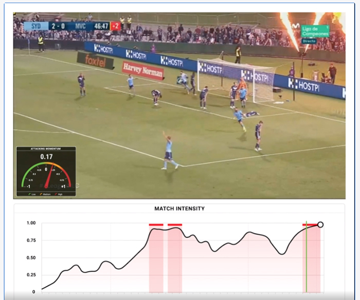
Watch the full video:
Model performance in production
Sportradar is investing in computer vision both through internal research, development, and external partnerships. To facilitate the rapid transition of computer vision models from the lab to production and running computer vision models at scale, Sportradar has developed a near-real-time computer vision inference pipeline using AWS services. The pipeline helps ensure that the service level agreements and low latency requirements for near-real-time computer vision workloads are met in a cost-effective way by using Amazon Elastic Kubernetes Service (Amazon EKS), Amazon Managed Streaming for Apache Kafka (Amazon MSK), and Amazon FSx for Lustre.
When deployed and tested in Sportradar’s computer vision inference pipeline, the latency for generating an inference from the goal prediction model featured in this article was around 200 milliseconds, with a total end-to-end processing latency of around 700 milliseconds.
Summary
Sportradar collaborated with the Amazon ML Solutions Lab to develop a novel computer vision-based Soccer Goal Predictor that predicts future goals with the precision of 75% while keeping the recall at 90%. We used transfer learning to fine-tune an I3D model in Amazon SageMaker to classify attacks that lead to goals as well as activities that don’t lead to goals, and used the model inference to create a momentum index to signal the intense moments in soccer. This model has been tested in Sportradar’s computer vision pipeline, and it can achieve close to real-time inference with low latency in sub-seconds. This approach can be applied to other sports in terms of key events prediction and game intensity measurement using computer vision infrastructure without relying on sensors for data collection.
If you’d like help accelerating the use of ML in your products and services, please contact the Amazon ML Solutions Lab program.
For more information about what the Amazon ML Solutions Lab is doing in the world of sports, see AWS Sports ML page.
About the Authors
 Daliana Zhen Liu a Senior Data Scientist at the Amazon ML Solutions Lab. She builds AI/ML solutions to help customers across various industries to accelerate their business. Previously, she worked at Amazon’s A/B testing platform helping retail teams make better data-driven decisions.
 Andrej Bratko leads a team of data scientists and engineers at Sportradar working on machine learning solutions in areas such as sports data collection, sportsbook risk management, odds trading and sports integrity. His team is also responsible for Sportradar’s big data and analytics infrastructure supporting machine learning model development and deployment. He holds a PhD in machine learning from the University of Ljubljana, Slovenia.
 Jure Prevc is a Data Scientist at Sportradar working mostly on risk management in sports betting. Besides his primary focus, he has a wide interest in different applications of machine learning and enjoys working on state-of-the-art solutions to solve complex business problems.
 Luka Pataky leads the Innovation Team at Sportradar – pioneering new technologies and products. One of the key innovation projects is computer vision, where he leads a team of data and computer vision engineers working on solutions to collect sports data and gather deeper insight into games. His team also works on other projects related to applying emerging technologies to products and processes, as well as projects that look at reinventing the way of how fans engage with sports and data.

Mehdi Noori is a Data Scientist at the Amazon ML Solutions Lab, where he works with customers across various verticals, and helps them to accelerate their cloud migration journey, and to solve their ML problems using state-of-the-art solutions and technologies.
 Suchitra Sathyanarayana is a manager at Amazon ML Solutions Lab, where she helps AWS customers across different industry verticals accelerate their AI and cloud adoption. She holds a PhD in Computer Vision from Nanyang Technological University, Singapore.
 Uros Lipovsek is machine learning engineer with experience in ML, computer vision, data engineering and devops. He is architecting computer vision pipeline at Sportradar and holds B.S. in Economics with focus on Econometrics from University of Ljubljana.
Amazon Scholar George Karypis receives ICDM 10-Year-Highest-Impact award
University of Minnesota professor and Amazon Scholar, together with coauthor, receives recognition for paper that proposes novel approach to algorithm that generates high-quality recommendations for e-commerce products at high speeds.Read More