Two of the world’s leading experts on algorithmic bias look back at the events of the past year and reflect on what we’ve learned, what we’re still grappling with, and how far we have to go.Read More
Automatically detecting personal protective equipment on persons in images using Amazon Rekognition
Workplace safety hazards can exist in many different forms: sharp edges, falling objects, flying sparks, chemicals, noise, and a myriad of other potentially dangerous situations. Safety regulators such as Occupational Safety and Health Administration (OSHA) and European Commission often require that businesses protect their employees and customers from hazards that can cause injury by providing personal protective equipment (PPE) and ensuring their use. Across many industries, such as manufacturing, construction, food processing, chemical, healthcare, and logistics, workplace safety is usually a top priority. In addition, due to the COVID-19 pandemic, wearing PPE in public places has become important to reduce the spread of the virus. In this post, we show you how you can use Amazon Rekognition PPE detection to improve safety processes by automatically detecting if persons in images are wearing PPE. We start with an overview of the PPE detection feature, explain how it works, and then discuss the different ways to deploy a PPE detection solution based on your camera and networking requirements.
Amazon Rekognition PPE detection overview
Even when people do their best to follow PPE guidelines, sometimes they inadvertently forget to wear PPE or don’t realize it’s required in the area they’re in. This puts their safety at potential risk and opens the business to possible regulatory compliance issues. Businesses usually rely on site supervisors or superintendents to individually check and remind all people present in the designated areas to wear PPE, which isn’t reliable, effective, or cost-efficient at scale. With Amazon Rekognition PPE detection, businesses can augment manual checks with automated PPE detection.
With Amazon Rekognition PPE detection, you can analyze images from your on-premises cameras at scale to automatically detect if people are wearing the required protective equipment, such as face covers (surgical masks, N95 masks, cloth masks), head covers (hard hats or helmets), and hand covers (surgical gloves, safety gloves, cloth gloves). Using these results, you can trigger timely alarms or notifications to remind people to wear PPE before or during their presence in a hazardous area to help improve or maintain everyone’s safety.
You can also aggregate the PPE detection results and analyze them by time and place to identify how safety warnings or training practices can be improved or generate reports for use during regulatory audits. For example, a construction company can check if construction workers are wearing head covers and hand covers when they’re on the construction site and remind them if one or more PPE isn’t detected to support their safety in case of accidents. A food processing company can check for PPE such as face covers and hand covers on employees working in non-contamination zones to comply with food safety regulations. Or a manufacturing company can analyze PPE detection results across different sites and plants to determine where they should add more hazard warning signage and conduct additional safety training.
With Amazon Rekognition PPE detection, you receive a detailed analysis of an image, which includes bounding boxes and confidence scores for persons (up to 15 per image) and PPE detected, confidence scores for the body parts detected, and Boolean values and confidence scores for whether the PPE covers the corresponding body part. The following image shows an example of PPE bounding boxes for head cover, hand covers, and face cover annotated using the analysis provided by the Amazon Rekognition PPE detection feature.
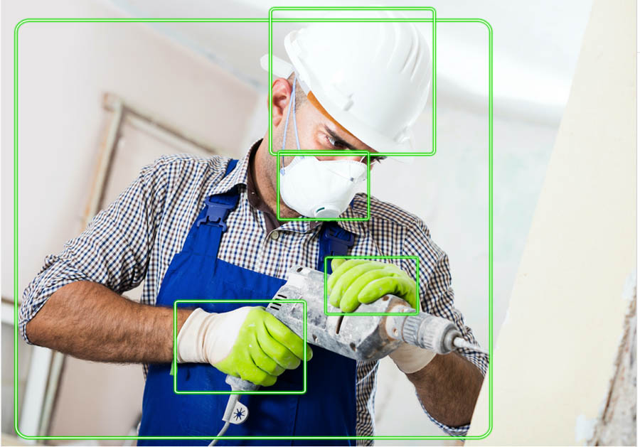
Often just detecting the presence of PPE in an image isn’t very useful. It’s important to detect if the PPE is worn by the customer or employee. Amazon Rekognition PPE detection also predicts a confidence score for whether the protective equipment is covering the corresponding body part of the person. For example, if a person’s nose is covered by face cover, head is covered by head cover, and hands are covered by hand covers. This prediction helps filter out cases where the PPE is in the image but not actually on the person.
You can also supply a list of required PPE (such as face cover or face cover and head cover) and a minimum confidence threshold (such as 80%) to receive a consolidated list of persons on the image that are wearing the required PPE, not wearing the required PPE, and when PPE can not be determined (such as when a body part isn’t visible). This reduces the amount of code developers need to write to high level counts or reference a person’s information in the image to further drill down.
Now, let’s take a closer look at how Amazon Rekognition PPE detection works.
How it works
To detect PPE in an image, you call the DetectProtectiveEquipment API and pass an input image. You can provide the input image (in JPG or PNG format) either as raw bytes or as an object stored in an Amazon Simple Storage Service (Amazon S3) bucket. You can optionally use the SummarizationAttributes (ProtectiveEquipmentSummarizationAttributes) input parameter to request summary information about persons that are wearing the required PPE, not wearing the required PPE, or are indeterminate.
The following image shows an example input image and its corresponding output from the DetectProtectiveEquipment as seen on the Amazon Rekognition PPE detection console. In this example, we supply face cover as the required PPE and 80% as the required minimum confidence threshold as part of summarizationattributes. We receive a summarization result that indicates that there are four persons in the image that are wearing face covers at a confidence score of over 80% [person identifiers 0, 1,2, 3]. It also provides the full fidelity API response in the per-person results. Note that this feature doesn’t perform facial recognition or facial comparison and can’t identify the detected persons.

Following is the DetectProtectiveEquipment API request JSON for this sample image in the console:
{
    "Image": {
        "S3Object": {
            "Bucket": "console-sample-images",
            "Name": "ppe_group_updated.jpg"
        }
    },
    "SummarizationAttributes": {
        "MinConfidence": 80,
        "RequiredEquipmentTypes": [
            "FACE_COVER"
        ]
    }
}
The response of the DetectProtectiveEquipment API is a JSON structure that includes up to 15 persons detected per image and for each person, the body parts detected (face, head, left hand, and right hand), the types of PPE detected, and if the PPE covers the corresponding body part. The full JSON response from DetectProtectiveEquipment API for this image is as follows:
"ProtectiveEquipmentModelVersion": "1.0",
"Persons": [
{
"BodyParts": [
{
"Name": "FACE",
"Confidence": 99.07738494873047,
"EquipmentDetections": [
{
"BoundingBox": {
"Width": 0.06805413216352463,
"Height": 0.09381836652755737,
"Left": 0.7537466287612915,
"Top": 0.26088595390319824
},
"Confidence": 99.98419189453125,
"Type": "FACE_COVER",
"CoversBodyPart": {
"Confidence": 99.76295471191406,
"Value": true
}
}
]
},
{
"Name": "LEFT_HAND",
"Confidence": 99.25702667236328,
"EquipmentDetections": []
},
{
"Name": "RIGHT_HAND",
"Confidence": 80.11490631103516,
"EquipmentDetections": []
},
{
"Name": "HEAD",
"Confidence": 99.9693374633789,
"EquipmentDetections": [
{
"BoundingBox": {
"Width": 0.09358207136392593,
"Height": 0.10753925144672394,
"Left": 0.7455776929855347,
"Top": 0.16204142570495605
},
"Confidence": 98.4826889038086,
"Type": "HEAD_COVER",
"CoversBodyPart": {
"Confidence": 99.99744415283203,
"Value": true
}
}
]
}
],
"BoundingBox": {
"Width": 0.22291666269302368,
"Height": 0.82421875,
"Left": 0.7026041746139526,
"Top": 0.15703125298023224
},
"Confidence": 99.97362518310547,
"Id": 0
},
{
"BodyParts": [
{
"Name": "FACE",
"Confidence": 99.71298217773438,
"EquipmentDetections": [
{
"BoundingBox": {
"Width": 0.05732834339141846,
"Height": 0.07323434203863144,
"Left": 0.5775181651115417,
"Top": 0.33671364188194275
},
"Confidence": 99.96135711669922,
"Type": "FACE_COVER",
"CoversBodyPart": {
"Confidence": 96.60395050048828,
"Value": true
}
}
]
},
{
"Name": "LEFT_HAND",
"Confidence": 98.09618377685547,
"EquipmentDetections": []
},
{
"Name": "RIGHT_HAND",
"Confidence": 95.69132995605469,
"EquipmentDetections": []
},
{
"Name": "HEAD",
"Confidence": 99.997314453125,
"EquipmentDetections": [
{
"BoundingBox": {
"Width": 0.07994530349969864,
"Height": 0.08479492366313934,
"Left": 0.5641391277313232,
"Top": 0.2394576370716095
},
"Confidence": 97.718017578125,
"Type": "HEAD_COVER",
"CoversBodyPart": {
"Confidence": 99.9454345703125,
"Value": true
}
}
]
}
],
"BoundingBox": {
"Width": 0.21979166567325592,
"Height": 0.742968738079071,
"Left": 0.49427083134651184,
"Top": 0.24296875298023224
},
"Confidence": 99.99588012695312,
"Id": 1
},
{
"BodyParts": [
{
"Name": "FACE",
"Confidence": 98.42090606689453,
"EquipmentDetections": [
{
"BoundingBox": {
"Width": 0.05756797641515732,
"Height": 0.07883334159851074,
"Left": 0.22534936666488647,
"Top": 0.35751715302467346
},
"Confidence": 99.97816467285156,
"Type": "FACE_COVER",
"CoversBodyPart": {
"Confidence": 95.9388656616211,
"Value": true
}
}
]
},
{
"Name": "LEFT_HAND",
"Confidence": 92.42487335205078,
"EquipmentDetections": []
},
{
"Name": "RIGHT_HAND",
"Confidence": 96.88029479980469,
"EquipmentDetections": []
},
{
"Name": "HEAD",
"Confidence": 99.98686218261719,
"EquipmentDetections": [
{
"BoundingBox": {
"Width": 0.0872764065861702,
"Height": 0.09496871381998062,
"Left": 0.20529428124427795,
"Top": 0.2652358412742615
},
"Confidence": 90.25578308105469,
"Type": "HEAD_COVER",
"CoversBodyPart": {
"Confidence": 99.99089813232422,
"Value": true
}
}
]
}
],
"BoundingBox": {
"Width": 0.19479165971279144,
"Height": 0.72265625,
"Left": 0.12187500298023224,
"Top": 0.2679687440395355
},
"Confidence": 99.98648071289062,
"Id": 2
},
{
"BodyParts": [
{
"Name": "FACE",
"Confidence": 99.32310485839844,
"EquipmentDetections": [
{
"BoundingBox": {
"Width": 0.055801939219236374,
"Height": 0.06405147165060043,
"Left": 0.38087061047554016,
"Top": 0.393160879611969
},
"Confidence": 99.98370361328125,
"Type": "FACE_COVER",
"CoversBodyPart": {
"Confidence": 98.56526184082031,
"Value": true
}
}
]
},
{
"Name": "LEFT_HAND",
"Confidence": 96.11709594726562,
"EquipmentDetections": []
},
{
"Name": "RIGHT_HAND",
"Confidence": 80.49284362792969,
"EquipmentDetections": []
},
{
"Name": "HEAD",
"Confidence": 99.91870880126953,
"EquipmentDetections": [
{
"BoundingBox": {
"Width": 0.08105235546827316,
"Height": 0.07952981442213058,
"Left": 0.36679577827453613,
"Top": 0.2875025272369385
},
"Confidence": 98.80988311767578,
"Type": "HEAD_COVER",
"CoversBodyPart": {
"Confidence": 99.6932144165039,
"Value": true
}
}
]
}
],
"BoundingBox": {
"Width": 0.18541666865348816,
"Height": 0.6875,
"Left": 0.3187499940395355,
"Top": 0.29218751192092896
},
"Confidence": 99.98927307128906,
"Id": 3
}
],
"Summary": {
"PersonsWithRequiredEquipment": [
0,
1,
2,
3
],
"PersonsWithoutRequiredEquipment": [],
"PersonsIndeterminate": []
}
}
Deploying Amazon Rekognition PPE detection
Depending on your use case, cameras, and environment setup, you can use different approaches to analyze your on-premises camera feeds for PPE detection. Because DetectProtectiveEquipment API only accepts images as input, you can extract frames from streaming or stored videos at the desired frequency (such as every 1, 2 or 5 seconds or every time motion is detected) and analyze those frames using the DetectProtectiveEquipment API. You can also set different frequencies of frame ingestion for cameras covering different areas. For example, you can set a higher frequency for busy or important locations and a lower frequency for areas that see light activity. This allows you to control the network bandwidth requirements because you only send images to the AWS cloud for processing.
The following architecture shows how you can design a serverless workflow to process frames from camera feeds for PPE detection.

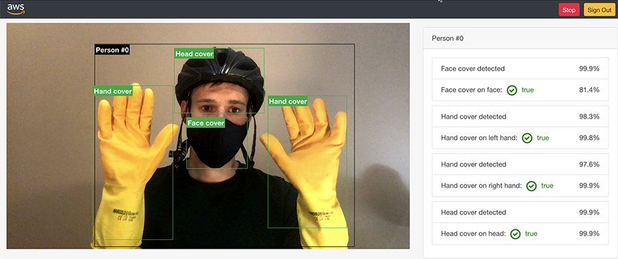
We have included a demo web application that implements this reference architecture in the Amazon Rekognition PPE detection GitHub repo. This web app extracts frames from a webcam video feed and sends them to the solution deployed in the AWS Cloud. As images get analyzed with the DetectProtectiveEquipment API, a summary output is displayed in the web app in near-real time. Following are a few example GIFs showing the detection of face cover, head cover, and hand covers as they are worn by a person in front of the webcam that is sampling a frame every two seconds. Depending on your use case, you can adjust the sampling rate to a higher or lower frequency. A screenshot showing the full demo application output, including the PPE and PPE worn or not predictions is also shown below.

Face cover detection

Hand cover detection

Head cover detection
Full demo web application output
Using this application and solution, you can generate notifications with Amazon Simple Notification Service. Although not implemented in the demo solution (but shown in the reference architecture), you can store the PPE detection results to create anonymized reports of PPE detection events using AWS services such as AWS Glue, Amazon Athena, and Amazon QuickSight. You can also optionally store ingested images in Amazon S3 for a limited time for regulatory auditing purposes. For instructions on deploying the demo web application and solution, see the Amazon Rekognition PPE detection GitHub repo.
Instead of sending images via Amazon API Gateway, you can also send images directly to an S3 bucket. This allows you to store additional metadata, including camera location, time, and other camera information, as Amazon S3 object metadata. As images get processed, you can delete them immediately or set them to expire within a time window using a lifecycle policy for an S3 bucket as required by your organization’s data retention policy. You can use the following reference architecture diagram to design this alternate workflow.

Extracting frames from your video systems
Depending on your camera setup and video management system, you can use the SDK provided by the manufacturer to extract frames. For cameras that support HTTP(s) or RTSP streams, the following code sample shows how you can extract frames at a desired frequency from the camera feed and process them using DetectProtectiveEquipment API.
import cv2
import boto3
import time
from datetime import datetime
import json

def processFrame(videoStreamUrl):
    cap = cv2.VideoCapture(videoStreamUrl)
    ret, frame = cap.read()
    if ret:
        hasFrame, imageBytes = cv2.imencode(".jpg", frame)
        if hasFrame:
            session = boto3.session.Session()
            rekognition = session.client('rekognition')
            response = rekognition. detect_protective_equipment(
                    Image={
                        'Bytes': imageBytes.tobytes(),
                    }
                )
            print(response)
    cap.release()

# Video stream
videoStreamUrl = "rtsp://@192.168.10.100"
frameCaptureThreshold = 300

while (True):
    try:
        processFrame(videoStreamUrl)
    except Exception as e:
        print("Error: {}.".format(e))

    time.sleep(frameCaptureThreshold)
To extract frames from stored videos, you can use AWS Elemental MediaConvert or other tools such as FFmpeg or OpenCV. The following code shows you how to extract frames from stored video and process them using the DetectProtectiveEquipment API:
import json
import boto3
import cv2
import math
import io

videoFile = "video file"
rekognition = boto3.client('rekognition')
ppeLabels = []
cap = cv2.VideoCapture(videoFile)
frameRate = cap.get(5) #frame rate
while(cap.isOpened()):
    frameId = cap.get(1) #current frame number
    print("Processing frame id: {}".format(frameId))
    ret, frame = cap.read()
    if (ret != True):
        break
    if (frameId % math.floor(frameRate) == 0):
        hasFrame, imageBytes = cv2.imencode(".jpg", frame)

        if(hasFrame):
            response = rekognition. detect_protective_equipment(
                Image={
                    'Bytes': imageBytes.tobytes(),
                }
            )

        for person in response["Persons"]:
            person["Timestamp"] = (frameId/frameRate)*1000
            ppeLabels.append(person)

print(ppeLabels)

with open(videoFile + ".json", "w") as f:
    f.write(json.dumps(ppeLabels))

cap.release()
Detecting other and custom PPE
Although the DetectProtectiveEquipment API covers the most common PPE, if your use case requires identifying additional equipment specific to your business needs, you can use Amazon Rekognition Custom Labels. For example, you can use Amazon Rekognition Custom Labels to quickly train a custom model to detect safety goggles, high visibility vests, or other custom PPE by simply supplying some labelled images of what to detect. No machine learning expertise is required to use Amazon Rekognition Custom Labels. When you have a custom model trained and ready for inference, you can then make parallel calls to DetectProtectiveEquipment and to the Amazon Rekognition Custom Labels model to detect all the required PPE and combine the results for further processing. For more information about using Amazon Rekognition Custom Labels to detect high-visibility vests including a sample solution with instructions, please visit the Custom PPE detection GitHub repository. You can use the following reference architecture diagram to design a combined DetectProtectiveEquipment and Amazon Rekognition Custom Labels PPE detection solution.

Conclusion
In this post, we showed how to use Amazon Rekognition PPE detection (the DetectProtectiveEquipment API) to automatically analyze images and video frames to check if employees and customers are wearing PPE such as face covers, hand covers, and head covers. We covered different implementation approaches, including frame extraction from cameras, stored video, and streaming videos. Finally, we covered how you can use Amazon Rekognition Custom Labels to identify additional equipment that is specific to your business needs.
To test PPE detection with your own images, sign in to the Amazon Rekognition console and upload your images in the Amazon Rekognition PPE detection console demo. For more information about the API inputs, outputs, limits, and recommendations, see Amazon Rekognition PPE detection documentation. To find out what our customers think about the feature or if you need a partner to help build an end-to-end PPE detection solution for your organization, see the Amazon Rekognition workplace safety web-page.
About the Authors
 Tushar Agrawal leads Outbound Product Management for Amazon Rekognition. In this role, he focuses on making customers successful by solving their business challenges with the right solution and go-to-market capabilities. In his spare time, he loves listening to music and re-living his childhood with his kindergartener.
 Kashif Imran is a Principal Solutions Architect at Amazon Web Services. He works with some of the largest AWS customers who are taking advantage of AI/ML to solve complex business problems. He provides technical guidance and design advice to implement computer vision applications at scale. His expertise spans application architecture, serverless, containers, NoSQL and machine learning.
 Matteo Figus is an AWS Solution Engineer based in the UK. Matteo works with the AWS Solution Architects to create standardized tools, code samples, demonstrations and quickstarts. He is passionate about open-source software and in his spare time he likes to cook and play the piano.
 Connor Kirkpatrick is an AWS Solution Engineer based in the UK. Connor works with the AWS Solution Architects to create standardised tools, code samples, demonstrations and quickstarts. He is an enthusiastic squash player, wobbly cyclist, and occasional baker.
A simpler singing synthesis system
New system is the first to use an attention-based sequence-to-sequence model, dispensing with separate models for features such as vibrato and phoneme durations.Read More
Detecting playful animal behavior in videos using Amazon Rekognition Custom Labels
Historically, humans have observed animal behaviors and applied them for different purposes. For example, behavioral observation is important in animal ecology, such as how often the behaviors are, when the behaviors occur, or whether there is individual difference or not. However, identifying and monitoring these behaviors and movements can be hard and can take a long time. To provide an automation for this workflow, a team from the agile members of pharmaceutical customer (Sumitomo Dainippon Pharma Co., Ltd.) and AWS Solutions Architects created a solution with Amazon Rekognition Custom Labels. Amazon Rekognition Custom Labels makes it easy to label specific movements in images, and train and build a model that detects these movements.
In this post, we show you how machine learning (ML) can help automate this workflow in a fun and simple way. We trained a custom model that detects playful behaviors of cats in a video using Amazon Rekognition Custom Labels. We hope to contribute to the afore-mentioned fields, biology and others by publicizing the architecture, our building process, and the source code for this solution.
About Amazon Rekognition Custom Labels
Amazon Rekognition Custom Labels is an automated ML feature that enables you to quickly train your own custom models for detecting business-specific objects and scenes from images—no ML experience required. For example, you can train a custom model to find your company logos in social media posts, identify your products on store shelves, or classify unique machine parts in an assembly line.
Amazon Rekognition Custom Labels builds off the existing capabilities of Amazon Rekognition, which is already trained on tens of millions of images across many categories. Instead of thousands of images, you simply need to upload a small set of training images (typically a few hundred images or less) that are specific to your use case. If your images are already labeled, Amazon Rekognition Custom Labels can begin training in just a few clicks. If not, you can label them directly within the Amazon Rekognition Custom Labels labeling interface, or use Amazon SageMaker Ground Truth to label them for you.
After Amazon Rekognition begins training from your image set, it can produce a custom image analysis model for you in just a few hours. Amazon Rekognition Custom Labels automatically loads and inspects the training data, selects the right ML algorithms, trains a model, and provides model performance metrics. You can then use your custom model via the Amazon Rekognition Custom Labels API and integrate it into your applications.
Solution overview
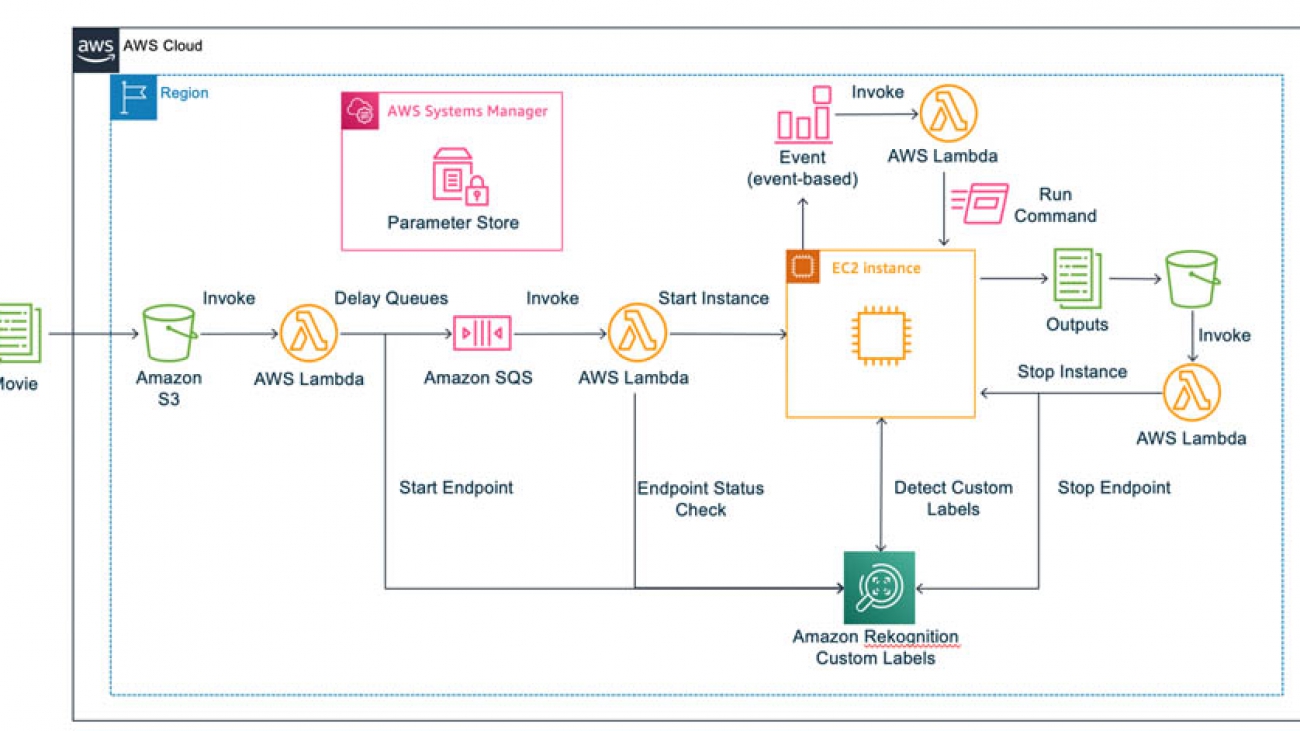
The following diagram shows the architecture of the solution. When you have model in place, the whole process of detecting specific behaviors in a video is automated; all you need to do is upload a video file (.mp4).

The workflow contains the following steps:
- You upload a video file (.mp4) to Amazon Simple Storage Service (Amazon S3), which invokes AWS Lambda, which in turn calls an Amazon Rekognition Custom Labels inference endpoint and Amazon Simple Queue Service (Amazon SQS). It takes about 10 minutes to launch the inference endpoint, so we use a deferred run of Amazon SQS.
- Amazon SQS invokes a Lambda function to do a status check of the inference endpoint, and launches Amazon Elastic Compute Cloud (Amazon EC2) if the status is
Running. - Amazon CloudWatch Events detects the
Runningstatus of Amazon EC2 and invokes a Lambda function, which runs a script on Amazon EC2 using the AWS Systems Manager Run - On Amazon EC2, the script calls the inference endpoint of Amazon Rekognition Custom Labels to detect specific behaviors in the video uploaded to Amazon S3 and writes the inferred results to the video on Amazon S3.
- When the inferred result file is uploaded to Amazon S3, a Lambda function launches to stop Amazon EC2 and the Amazon Rekognition Custom Labels inference endpoint.
Prerequisites
For this walkthrough, you should have the following prerequisites:
- An AWS account – You can create a new account if you don’t have one yet.
- A key pair – You need a key pair to log in to the EC2 instance that uses Amazon Rekognition Custom Labels to detect specific behaviors. You can either use an existing key pair or create a new key pair. For more information, see Amazon EC2 key pairs and Linux instances.
- A video for inference – This solution uses a video (.mp4 format) for inference. You can use your own video or the one we provide in this post.
Launching your AWS CloudFormation stack
Launch the provided AWS CloudFormation
After you launch the template, you’re prompted to enter the following parameters:
- KeyPair – The name of the key pair used to connect to the EC2 instance
- ModelName – The model name used for Amazon Rekognition Custom Labels
- ProjectARN – The project ARN used for Amazon Rekognition Custom Labels
- ProjectVersionARN – The model version name used for Amazon Rekognition Custom Labels
- YourCIDR – The CIDR including your public IP address

For this post, we use the following video to detect whether a cat is punching or not. For our object detection model, we prepared an annotated dataset and trained it in advance, as shown in the following section.
This solution uses the US East (N. Virginia) Region, so make sure to work in that Region when following along with this post.
Adding annotations to images from the video
To annotate your images, complete the following steps:
- To create images that the model uses for learning, you need to split the video into a series of still images. For this post, we prepared 377 images (the ratio of normal videos to punching videos is about 2:1) and annotated them.
- Store the series of still images in Amazon S3 and annotate them. You can use Ground Truth to annotate them.
- Because we’re creating an object detection model, select Bounding box for the Task type.
- For our use case, we want to tell if a cat is punching or not in the video, so we create a labeling job using two labels:
normalto define basic sitting behavior, andpunchto define playful behavior. - For annotation, you should surround the cat with the
normallabel bounding box when the cat isn’t punching, and surround the cat with thepunchlabel bounding box when the cat is punching.
When the cat is punching, the image of the cat’s paws should look blurred, so based on how blurred the image is, you can determine whether the cat is punching or not and annotate the image.

Training a custom ML model
To start training your model, complete the following steps:
- Create an object detection model using Amazon Rekognition Custom Labels. For instructions, see Getting Started with Amazon Rekognition Custom Labels.
- When you create a dataset, choose Import images labeled by SageMaker Ground Truth for Image location
- Set the
output.manifestfile path that was output by the Ground Truth labeling job.
To find the path out the output.manifest file, on the Amazon SageMaker console, on the Labeling jobs page, choose your video. The information is located on the Labeling job summary page.

- When the model has finished learning, save the ARN listed in the Use your model section at the bottom of the model details page. We use this ARN later on.

For reference, the F1 score for normal and punch was above 0.9 in our use case.
Uploading a video for inference on Amazon S3
You can now upload your video for inference.
- On the Amazon S3 console, navigate to the bucket you created with the CloudFormation stack (it should include
rekognitionin the name). - Choose Create folder.
- Create the folder
inputMovie. - Upload the file you want to infer.

Setting up a script on Amazon EC2
This solution calls the Amazon Rekognition API to infer the video on Amazon EC2, so you need to set up a script on Amazon EC2.
- Log in to Amazon EC2 via SSH with the following code and the key pair you created:
ssh -i <Your key Pair> ubuntu@<EC2 IPv4 Public IP>
Are you sure you want to continue connecting (yes/no)? yes
Welcome to Ubuntu 18.04.4 LTS (GNU/Linux 4.15.0-1065-aws x86_64)
ubuntu@ip-10-0-0-207:~$ cd code/
ubuntu@ip-10-0-0-207:~/code$ vi rekognition.py
It takes approximately 30 minutes to install and build the necessary libraries.
- Copy the following code to
rekognition.pyand replace <BucketName> with your S3 bucket name created by AWS CloudFormation. This code uses OpenCV to split the video into frames and throws each frame to the inference endpoint of Amazon Rekognition Custom Labels to perform behavior detection. It merges the inferred behavior detection result with each frame and puts the frames together to reconstruct a video.
import boto3
import cv2
import json
from decimal import *
import os
import ffmpeg

def get_parameters(param_key):
    ssm = boto3.client('ssm', region_name='us-east-1')
    response = ssm.get_parameters(
        Names=[
            param_key,
        ]
    )
    return response['Parameters'][0]['Value']

def analyzeVideo():
    ssm = boto3.client('ssm',region_name='us-east-1')
    s3 = boto3.resource('s3')
    rekognition = boto3.client('rekognition','us-east-1')

    parameter_value = get_parameters('/Movie/<BucketName>')
    dirname, video = os.path.split(parameter_value)
    bucket = s3.Bucket('<BucketName>')
    bucket.download_file(parameter_value, video)

    customLabels = []
    cap = cv2.VideoCapture(video)
    frameRate = cap.get(cv2.CAP_PROP_FPS)
    width = cap.get(cv2.CAP_PROP_FRAME_WIDTH)
    height = cap.get(cv2.CAP_PROP_FRAME_HEIGHT)
    fourcc = cv2.VideoWriter_fourcc(*'XVID')
    writer = cv2.VideoWriter( video + '-output.avi', fourcc, 18, (int(width), int(height)))

    while(cap.isOpened()):
        frameId = cap.get(cv2.CAP_PROP_POS_FRAMES)
        print(frameId)
        print("Processing frame id: {}".format(frameId))
        ret, frame = cap.read()
        if (ret != True):
            break
        hasFrame, imageBytes = cv2.imencode(".jpg", frame)

        if(hasFrame):
            response = rekognition.detect_custom_labels(
                Image={
                    'Bytes': imageBytes.tobytes(),
                },
                ProjectVersionArn = get_parameters('ProjectVersionArn')
            )

            for output in response["CustomLabels"]:
                Name = output['Name']
                Confidence = str(output['Confidence'])
                w = output['Geometry']['BoundingBox']['Width']
                h = output['Geometry']['BoundingBox']['Height']
                left = output['Geometry']['BoundingBox']['Left']
                top = output['Geometry']['BoundingBox']['Top']
                w = int(w * width)
                h = int(h * height)
                left = int(left*width)
                top = int(top*height)

                output["Timestamp"] = (frameId/frameRate)*1000
                customLabels.append(output)
                if Name == 'Moving':
                    cv2.rectangle(frame,(left,top),(left+w,top+h),(0,0,255),2)
                    cv2.putText(frame,Name + ":" +Confidence +"%",(left,top),cv2.FONT_HERSHEY_SIMPLEX,0.5,(0, 0, 255), 1, cv2.LINE_AA)
                else:
                    cv2.rectangle(frame,(left,top),(left+w,top+h),(0,255,0),2)
                    cv2.putText(frame,Name + ":" +Confidence +"%",(left,top),cv2.FONT_HERSHEY_SIMPLEX,0.5,(0, 255, 0), 1, cv2.LINE_AA)

        writer.write(frame)
    print(customLabels)

    with open(video + ".json", "w") as f:
        f.write(json.dumps(customLabels))
    bucket.upload_file(video + ".json",'output-json/ec2-output.json')
    stream = ffmpeg.input(video + '-output.avi')
    stream = ffmpeg.output(stream, video + '-output.mp4', pix_fmt='yuv420p', vcodec='libx264')
    stream = ffmpeg.overwrite_output(stream)
    ffmpeg.run(stream)
    bucket.upload_file( video + '-output.mp4','output/' +video + '-output.mp4')

    writer.release()
    cap.release()

analyzeVideo()
Stopping the EC2 instance
Stop the EC2 instance after you create the script in it. The EC2 instance is automatically launched when a video file is uploaded to Amazon S3.

The solution is now ready for use.
Detecting movement in the video
To implement your solution, upload a video file (.mp4) to the inputMovie folder you created. This launches the endpoint for Amazon Rekognition Custom Labels.

When the status of the endpoint changes to Running, Amazon EC2 launches and performs behavior detection. A video containing behavior detection data is uploaded to the output folder in Amazon S3.
When you log in to Amazon EC2, you can see that a video file that merged the inferred results was created under the code folder.

The video file is stored in the output folder created in Amazon S3. This causes the endpoint for Amazon Rekognition Custom Labels and Amazon EC2 to stop.

The following video is the result of detecting a specific movement (punch) of the cat:
Cleaning Up
To avoid incurring future charges, delete the resources you created.
Conclusion and next steps
This solution automates detecting specific actions in a video. In this post, we created a model to detect specific cat behaviors using Amazon Rekognition Custom Labels, but you can also use custom labels to identify cell images (such data is abundant in the research field). For example, the following screenshot shows the inferred results of a model that learned leukocytes, erythrocytes, and platelets. We had the model learn from 20 datasets, and it can now detect cells with distinctive features that are identifiable with human eyes. Its accuracy can increase as more high-resolution data is added and as annotations are done more carefully.

Amazon Rekognition Custom Labels has a wide range of use cases in the research field. If you want to try this in your organization and have any questions, please reach out to us or your Solutions Architects team and they will be excited to assist you.
About the Authors
 Hidenori Koizumi is a Solutions Architect in Japan’s Healthcare and Life Sciences team. He is good at developing solutions in the research field based on his scientific background (biology, chemistry, and more). His specialty is machine learning, and he has recently been developing applications using React and TypeScript. His hobbies are traveling and photography.
 Mari Ohbuchi is a Machine Learning Solutions Architect at Amazon Web Services Japan. She worked on developing image processing algorithms for about 10 years at a manufacturing company before joining AWS. In her current role, she supports the implementation of machine learning solutions and creating prototypes for manufacturing and ISV/SaaS customers. She is a cat lover and has published blog posts, hands-on content, and other content that involves both AWS AI/ML services and cats.
Processing auto insurance claims at scale using Amazon Rekognition Custom Labels and Amazon SageMaker Ground Truth
Computer vision uses machine learning (ML) to build applications that process images or videos. With Amazon Rekognition, you can use pre-trained computer vision models to identify objects, people, text, activities, or inappropriate content. Our customers have use cases that span every industry, including media, finance, manufacturing, sports, and technology. Some of these use cases require training custom computer vision models to detect business-specific objects. When building custom computer vision models, customers tell us they face two main challenges: availability of labeled training data, and accessibility to resources with ML expertise.
In this post, I show you how to mitigate these challenges by using Amazon SageMaker Ground Truth to easily build a training dataset from unlabeled data, followed by Amazon Rekognition Custom Labels to train a custom computer vision model without requiring ML expertise.
For this use case, we want to build a claims processing application for motor vehicle insurance that allows customers to submit an image of their vehicle with their insurance claim. Customers might accidentally submit a wrong picture, and some may try to commit fraud by submitting false pictures. Various ML models can fully or partially automate the processing of these images and the rest of the claim contents. This post walks through the steps required to train a simple computer vision model that detects if images are relevant to vehicle insurance claims or not.
Services overview
Amazon Rekognition Custom Labels is an automated machine learning (AutoML) feature that enables you to train custom ML models for image analysis without requiring ML expertise. Upload a small dataset of labeled images specific to your business use case, and Amazon Rekognition Custom Labels takes care of the heavy lifting of inspecting the data, selecting an ML algorithm, training a model, and calculating performance metrics.
Amazon Rekognition Custom Labels provides a UI for viewing and labeling a dataset on the Amazon Rekognition console, suitable for small datasets. It also supports auto-labeling based on the folder structure of an Amazon Simple Storage Service (Amazon S3) bucket, and importing labels from a Ground Truth output file. Ground Truth is the recommended labeling tool when you have a distributed labeling workforce, need to implement a complex labeling pipeline, or have a large dataset.
Ground Truth is a fully managed data labeling service used to easily and efficiently build accurate datasets for ML. It provides built-in workflows to label image, text, and 3D point cloud data, and supports custom workflows for other types of data. You can set up a public or private workforce, and take advantage of automatic data labeling to reduce the time required to label the dataset.
Solution overview
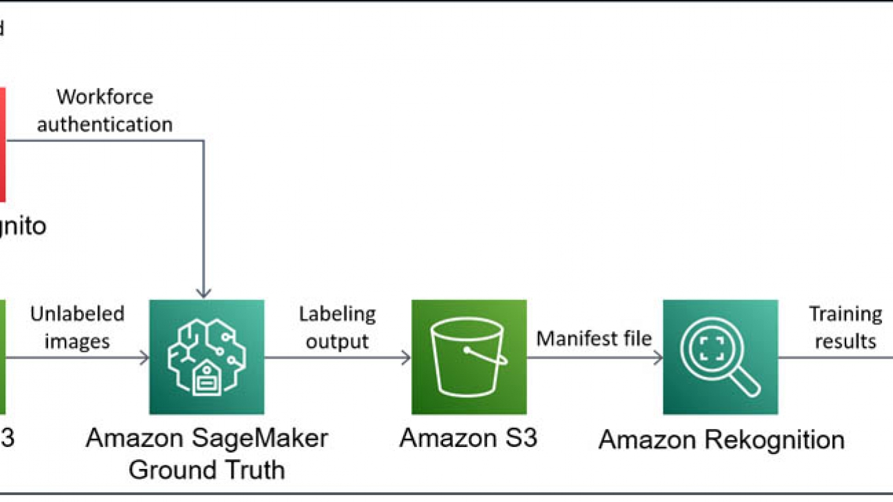
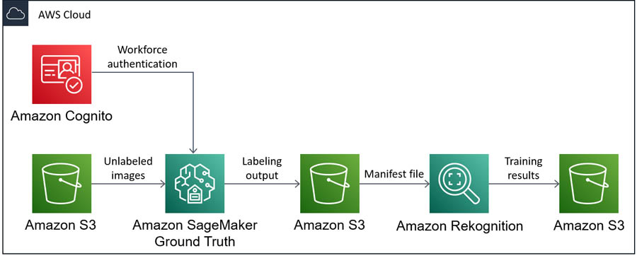
The core of the solution is Ground Truth and Amazon Rekognition Custom Labels, but you also use S3 buckets to store data between each step. You first need an S3 bucket to store unlabeled images. Then, you set up a labeling job in Ground Truth for the image data in the bucket, using Amazon Cognito to authenticate users for your private workforce. Ground Truth saves the labeling results in another S3 bucket as a manifest file, which is used to build training and test datasets in Amazon Rekognition Custom Labels. Finally, you can train a custom model using your new dataset in Amazon Rekognition Custom Labels, the results of which are saved in another S3 bucket.
The following diagram illustrates the architecture of this solution.
Detailed walkthrough
In this post, I show you how to train a custom computer vision model to detect if images are relevant to vehicle insurance claims. These steps are as follows:
- Collect data
- Label the data
- Train the computer vision model
- Evaluate the computer vision model
Before you start collecting data, you need decide which type of computer vision model to use. At the time of writing, Amazon Rekognition Custom Labels supports two computer vision models:
- Image classification – Assigns labels to an image as a whole
- Object detection – Draws bounding boxes around objects of interest in an image
Object detection is more specific than image classification, but labeling images for object detection also requires more time and effort, so it’s important to consider the requirements of the use case.
For this use case, I start by building a model to detect the difference between images with a vehicle and images without a vehicle. At this point, I’m not interested in knowing exactly where the vehicle is located on the image, so I can start with image classification.
Prerequisites
To successfully follow the steps in this walkthrough, you need to complete the following prerequisites:
- Create an AWS account.
- Create an AWS Identity and Access Management (IAM) user with AWS Management Console access and programmatic access. For instructions, see Creating an IAM User in Your AWS Account.
- Assign permissions to the IAM user that allow the user to create new resources and use the services referred to in this post. I recommend the following managed policies:
AmazonSageMakerFullAccessAmazonRekognitionCustomLabelsFullAccessAmazonCognitoPowerUserAmazonS3FullAccessIAMFullAccess
- Install and configure the AWS Command Line Interface (AWS CLI) on your local machine. For instructions, see Installing, updating, and uninstalling the AWS CLI version 2.
In this post, I demonstrate how to build the full solution using the AWS CLI, which allows you to programmatically create, manage, and monitor AWS resources from a terminal. The AWS CLI supports all AWS services and can be used to automate your cloud infrastructure. If you prefer to use the console, I provide links to console instructions in each section.
Collecting data
First, you need to collect relevant images. Ideally, I would source these images from actual images submitted by insurance customers, which are representative of what the model sees in production. However, for this post, I use images from the COCO (Common Objects in Context) dataset. This is a large dataset of everyday images where common objects have been labeled with semantic segmentation, captions, and keypoints.
The original COCO dataset from 2017 is up to 26 GB in size and can take a long time to download. This walkthrough only relies on a small subset of images from the dataset, so you can download the COCO subset (3 GB) provided by the fast.ai research group instead. You can complete the data collection steps on your local machine, an Amazon Elastic Compute Cloud (Amazon EC2) instance, an Amazon SageMaker Jupyter notebook, or any other compute resource.
- Enter the following code to download the dataset:
wget https://s3.amazonaws.com/fast-ai-coco/coco_sample.tgz- When the download is complete, extract the .tgz file:
tar -xvzf coco_sample.tgzYou now have a directory called coco_sample, with two sub-directories: annotations and train_sample. The COCO dataset already provides labels for various vehicles and other objects in the images, but you can ignore these for this use case, because you want to use Ground Truth for labeling.
- Navigate to the directory that contains only the images:
cd ./coco_sample/train_sampleEven though this is only a subset of the COCO dataset, this directory still contains 21,837 images. For this use case, I spent some time looking through the images in this dataset to collect the file names of images that contain vehicles. I then took a random sample of file names from the remaining images to create a dataset of images without vehicles.
- To use the same images, copy the file names into a text file using the following code:
echo "000000000723.jpg 000000057387.jpg 000000121555.jpg 000000175523.jpg 000000280926.jpg 000000482049.jpg 000000000985.jpg 000000060548.jpg 000000128015.jpg 000000179251.jpg 000000296696.jpg 000000498570.jpg 000000004764.jpg 000000067222.jpg 000000131465.jpg 000000184543.jpg 000000302415.jpg 000000509657.jpg 000000005965.jpg 000000068668.jpg 000000135438.jpg 000000185262.jpg 000000303590.jpg 000000515020.jpg 000000007713.jpg 000000068801.jpg 000000136185.jpg 000000188440.jpg 000000306415.jpg 000000517921.jpg 000000016593.jpg 000000069577.jpg 000000137475.jpg 000000190026.jpg 000000318496.jpg 000000540547.jpg 000000020289.jpg 000000077837.jpg 000000140332.jpg 000000190447.jpg 000000318672.jpg 000000543058.jpg 000000024396.jpg 000000078407.jpg 000000142847.jpg 000000195538.jpg 000000337265.jpg 000000547345.jpg 000000025453.jpg 000000079481.jpg 000000144992.jpg 000000197792.jpg 000000337638.jpg 000000553862.jpg 000000026992.jpg 000000079873.jpg 000000146907.jpg 000000206539.jpg 000000341429.jpg 000000557155.jpg 000000028333.jpg 000000081315.jpg 000000148165.jpg 000000213342.jpg 000000341902.jpg 000000557819.jpg 000000030001.jpg 000000084171.jpg 000000158130.jpg 000000217043.jpg 000000361140.jpg 000000560123.jpg 000000033505.jpg 000000093070.jpg 000000159280.jpg 000000219762.jpg 000000361255.jpg 000000561126.jpg 000000035382.jpg 000000099453.jpg 000000164178.jpg 000000237031.jpg 000000375500.jpg 000000566364.jpg 000000039100.jpg 000000104844.jpg 000000168817.jpg 000000241279.jpg 000000375654.jpg 000000571584.jpg 000000043270.jpg 000000109738.jpg 000000170784.jpg 000000247473.jpg 000000457725.jpg 000000573286.jpg 000000047425.jpg 000000111889.jpg 000000171970.jpg 000000250955.jpg 000000466451.jpg 000000576449.jpg 000000049006.jpg 000000120021.jpg 000000173001.jpg 000000261479.jpg 000000468652.jpg 000000053580.jpg 000000121162.jpg 000000174911.jpg 000000264016.jpg 000000479219.jpg" > vehicle-images.txtThe dataset contains many more images featuring vehicles, but this subset of 56 images (plus 56 non-vehicle images) should be sufficient to demonstrate the full pipeline for training a custom computer vision model.
- To store this subset of images, create a new directory:
mkdir vehicle_dataset- Using the text file containing the image file names, copy the relevant images into the new directory:
xargs -a ./vehicle-images.txt cp -t ./vehicle_datasetYou now have an unlabeled dataset on your local computer that you can use to build your model.
You can now create a new S3 bucket in your AWS account and upload your images into this bucket. At this point, it’s important to choose the Region where you want to deploy the resources. Use the Region Table to choose a Region that supports Amazon Rekognition Custom Labels and Ground Truth. I use us-west-2, but if you want to use a different Region, adjust the --region flag in the following CLI commands. You can also create a bucket and upload the dataset on the console.
- First, create an S3 bucket with a unique name. Replace <BUCKET_NAME> with a bucket name of your choice:
aws s3 mb s3://<BUCKET_NAME> --region us-west-2- Copy the data from your local computer into your new S3 bucket:
aws s3 cp ./vehicle_dataset s3://<BUCKET_NAME>/imgs/ --recursiveLabeling the data
After you successfully upload the unlabeled images to your S3 bucket, you use Ground Truth to label the data. This service is designed to help you build highly accurate training datasets for ML. For more information, see Use Amazon SageMaker Ground Truth to Label Data or the AWS Blog.
To create your dataset of labeled vehicle images, you complete three steps:
- Create a workforce
- Set up a labeling job
- Complete the labeling task
Creating a workforce
There are several options for setting up a workforce of annotators in Ground Truth:
- A crowdsourced workforce using Amazon Mechanical Turk
- A private workforce of your own internal resources
- A workforce provided by one of the curated third-party vendors on AWS Marketplace
Because this use case is small (only 112 images), you can complete the task yourself by setting up a private workforce. In this post, I show you how to set up a private workforce using the AWS CLI. For instructions on setting up your workforce on the console, see the section Creating a labeling workforce in the post Amazon SageMaker Ground Truth – Build Highly Accurate Datasets and Reduce Labeling Costs by up to 70%. Alternatively, see Create a Private Workforce (Amazon SageMaker Console).
For more information about using the AWS CLI and the commands in this section, see the following:
- First, create an Amazon Cognito user pool:
aws cognito-idp create-user-pool
--pool-name vehicle-experts-user-pool
--region us-west-2
- Record the Id value in the output. This should have a format similar to
us-west-2_XXXXXXXXX. - Create a user group in the user pool. Replace the value for <USER_POOL_ID> with the ID value you recorded in the previous step:
aws cognito-idp create-group
--group-name vehicle-experts-user-group
--user-pool-id <USER_POOL_ID>
--region us-west-2
- Create a user pool client:
aws cognito-idp create-user-pool-client
--user-pool-id <USER_POOL_ID>
--client-name vehicle-experts-user-pool-client
--generate-secret
--explicit-auth-flows ALLOW_CUSTOM_AUTH ALLOW_USER_PASSWORD_AUTH ALLOW_USER_SRP_AUTH ALLOW_REFRESH_TOKEN_AUTH
--supported-identity-providers COGNITO
--region us-west-2
- Record the ClientId value in the output.
- Create a user pool domain:
aws cognito-idp create-user-pool-domain
--domain vehicle-experts-user-pool-domain
--user-pool-id <USER_POOL_ID>
--region us-west-2
- Create a work team for Ground Truth. Replace the values for <USER_POOL_ID> and <USER_POOL_CLIENT_ID> with the user pool ID and the user pool client ID, respectively. If you used a different name for your user group than
vehicle-experts-user-group, replace this value as well.
aws sagemaker create-workteam
--workteam-name vehicle-experts-workteam
--member-definitions '{"CognitoMemberDefinition": {"UserPool": "<USER_POOL_ID>", "UserGroup": "vehicle-experts-user-group", "ClientId": "<USER_POOL_CLIENT_ID>"}}'
--description "A team of vehicle experts"
--region us-west-2
- Record the WorkteamARN value in the output.
After you create a work team in Amazon SageMaker, update the user pool client to allow for OAuth flows and scopes. To complete this step, you need to find the callback URL and the logout URL generated during the creation of the work team.
- Find the URLs with the following code:
aws cognito-idp describe-user-pool-client
--user-pool-id <USER_POOL_ID>
--client-id <USER_POOL_CLIENT_ID>
--region us-west-2
- Make a note of the URL in the CallbackURLs list, which should look similar to
https://XXXXXXXXXX.labeling.us-west-2.sagemaker.aws/oauth2/idpresponse. - Also make a note of the URL in the LogoutURLs list, which should look similar to
https://XXXXXXXXXX.labeling.us-west-2.sagemaker.aws/logout. - Use these URLs to update the user pool client:
aws cognito-idp update-user-pool-client
--user-pool-id <USER_POOL_ID>
--client-id <USER_POOL_CLIENT_ID>
--allowed-o-auth-flows-user-pool-client
--allowed-o-auth-scopes email openid profile
--allowed-o-auth-flows code implicit
--callback-urls '["<CALLBACK_URL>"]'
--logout-urls '["<LOGOUT_URL>"]'
--supported-identity-providers COGNITO
--region us-west-2
You should now be able to access the labeling portal sign-in screen by navigating to the root of the callback and logout URLs (http://XXXXXXXXXX.labeling.us-west-2.sagemaker.aws). If you want to create any more Amazon SageMaker work teams in this Region in the future, you only need to create a new user pool group and a new work team.
You now have a work team without any workers, and need to add some.
- Add yourself as a worker using the following code:
aws cognito-idp admin-create-user
--user-pool-id <USER_POOL_ID>
--username the_vehicle_expert
--user-attributes '[{"Name": "email", "Value": "<EMAIL_ADDRESS>"}]'
--region us-west-2
It’s important to provide a valid email address because Amazon Cognito sends an email with your username and temporary password. You use these credentials to log in to the labeling portal, and you must change your password when you log in for the first time.
- Add your user to the user group created within the user pool, because labeling jobs in Ground Truth are assigned to user pool groups. Replace the value of <USER_POOL_ID> with the ID of your user pool. If you used a different name for your user group than
vehicle-experts-user-group, replace this value as well.
aws cognito-idp admin-add-user-to-group
--user-pool-id <USER_POOL_ID>
--username the_vehicle_expert
--group-name vehicle-experts-user-group
--region us-west-2
If you forget this step, you can log in to the labeling portal, but you aren’t assigned any labeling tasks.
Setting up a labeling job
You can now set up the labeling job in Ground Truth. In this post, I demonstrate how to set up a labeling job using the AWS CLI. For instructions on setting up your workforce on the console, see the section Creating a labeling job in the post Amazon SageMaker Ground Truth – Build Highly Accurate Datasets and Reduce Labeling Costs by up to 70%. Be careful to choose the image classification task type instead of the bounding box task type. Alternatively, see Create a Labeling Job.
For more information about using the AWS CLI and the commands in this section, see the following:
- AWS CLI Command Reference
- Amazon SageMaker API Reference
- Amazon S3 REST API Introduction
- IAM API Reference
To create a labeling job in Ground Truth, you need to create a manifest file that points to the location of your unlabeled images. After labeling is complete, Ground Truth generates a new version of this manifest file with the labeling results added. A manifest file is a JSON lines file with a well-defined structure. For the input manifest file for Ground Truth, each JSON object only requires the source-ref key. The console has an option to have Ground Truth generate the manifest file for you. However, you can generate the manifest file with one piece of code, using the images.txt file created earlier.
- Generate the manifest file with the following code:
cat vehicle-images.txt | tr ' ' 'n' | awk '{print "{"source-ref":"s3://<BUCKET_NAME>/imgs/" $0 ""}"}' > vehicle-dataset.manifest- Upload this manifest file to a new directory in your S3 bucket:
aws s3 cp ./vehicle-dataset.manifest s3://<BUCKET_NAME>/groundtruth-input/You need to create a template for the labeling UI that the annotators (for this use case, you) use to label the data. To create this UI template, I use the image classification UI sample from the Amazon SageMaker Ground Truth Sample Task UIs GitHub repo, and edit the text to represent this use case. You can save the following template in a file called template.liquid on your local machine.
- Create and save the template with the following code:
<script src="https://assets.crowd.aws/crowd-html-elements.js"></script>

<crowd-form>
  <crowd-image-classifier
    name="crowd-image-classifier"
    src="{{ task.input.taskObject | grant_read_access }}"
    header="If the image contains a vehicle in plain sight, assign the 'vehicle' label. Otherwise, assign the 'other' label."
    categories="{{ task.input.labels | to_json | escape }}"
  >
    <full-instructions header="Classification Instructions">
      <p>Read the task carefully and inspect the image.</p>
      <p>Choose the appropriate label that best suits the image.</p>
    </full-instructions>

    <short-instructions>
      <p>Read the task carefully and inspect the image.</p>
      <p>Choose the appropriate label that best suits the image.</p>
    </short-instructions>
  </crowd-image-classifier>
</crowd-form>
- Upload this UI template to your S3 bucket:
aws s3 cp ./template.liquid s3://<BUCKET_NAME>/groundtruth-input/Ground Truth expects a file that specifies the labels the annotators can assign to objects in the images. For this use case, you define two labels: vehicle and other. This label category configuration file is a JSON file with a simple structure as shown in the following code. You can save the template in a file called data.json on your local machine.
- Define the labels with the following code:
{"document-version":"2018-11-28","labels":[{"label":"vehicle"},{"label":"other"}]}- As with the manifest file before, upload the label category configuration to the S3 bucket:
aws s3 cp ./data.json s3://<BUCKET_NAME>/groundtruth-input/For certain image tasks, the S3 bucket where the data is stored must have CORS settings enabled. You can do this with the following CLI command:
aws s3api put-bucket-cors
--bucket <BUCKET_NAME>
--cors-configuration '{"CORSRules": [{"AllowedMethods": ["GET"], "AllowedOrigins": ["*"]}]}'
Ground Truth needs to be assigned an IAM role that allows it to perform necessary actions and access the S3 bucket containing the data. Create a new IAM service role for Amazon SageMaker with a maximum session duration longer than the default value. You set a task time limit for the labeling job later, and the maximum session duration for the IAM role needs to be larger than or equal to this task time limit.
- Create the role with the following code:
aws iam create-role
--role-name SageMakerGroundTruthRole
--assume-role-policy-document '{"Version": "2012-10-17", "Statement": {"Effect": "Allow", "Principal": {"Service": "sagemaker.amazonaws.com"}, "Action": "sts:AssumeRole"}}'
--max-session-duration 36000
- Make a note of the
Arnvalue in the output. - Attach the
AmazonSageMakerFullAccessmanaged policy to this role:
aws iam attach-role-policy
--role-name SageMakerGroundTruthRole
--policy-arn arn:aws:iam::aws:policy/AmazonSageMakerFullAccess
- Create a new IAM policy that allows read and write access to the S3 bucket containing the data input for Ground Truth:
aws iam create-policy
--policy-name AccessVehicleDatasetBucket
--policy-document '{"Version": "2012-10-17", "Statement": [{"Effect": "Allow", "Action": ["s3:GetObject", "s3:PutObject", "s3:GetBucketLocation", "s3:ListBucket"], "Resource": ["arn:aws:s3:::<BUCKET_NAME>/*"]}]}'
- Make a note of the
Arnvalue in the output. - Attach your new policy to the IAM role. Replace <POLICY_ARN> with the ARN value copied from the output of the previous command:
aws iam attach-role-policy
--role-name SageMakerGroundTruthRole
--policy-arn <POLICY_ARN>
You can now create the labeling job. This is a large CLI command compared to the earlier ones. You need to provide the Amazon S3 URIs for the manifest file, the output directory, the label category configuration file, and the UI template. Replace <BUCKET_NAME> with your chosen bucket name in each URI. Replace <ROLE_ARN> with the ARN value copied from the output of the create-role command, and replace <WORKTEAM_ARN> with the ARN value copied from the output of the create-workteam command.
- Create the labeling job with the following code:
aws sagemaker create-labeling-job
--labeling-job-name vehicle-labeling-job
--label-attribute-name vehicle
--input-config '{"DataSource": {"S3DataSource": {"ManifestS3Uri": "s3://<BUCKET_NAME>/groundtruth-input/vehicle-dataset.manifest"}}}'
--output-config '{"S3OutputPath": "s3://<BUCKET_NAME>/groundtruth-output/"}'
--role-arn <ROLE_ARN>
--label-category-config-s3-uri s3://<BUCKET_NAME>/groundtruth-input/data.json
--human-task-config '{"WorkteamArn": "<WORKTEAM_ARN>", "UiConfig": {"UiTemplateS3Uri": "s3://<BUCKET_NAME>/groundtruth-input/template.liquid"}, "PreHumanTaskLambdaArn": "arn:aws:lambda:us-west-2:081040173940:function:PRE-ImageMultiClass", "TaskTitle": "Vehicle labeling task", "TaskDescription": "Assign a label to each image based on the presence of vehicles in the image.", "NumberOfHumanWorkersPerDataObject": 1, "TaskTimeLimitInSeconds": 600, "AnnotationConsolidationConfig": {"AnnotationConsolidationLambdaArn": "arn:aws:lambda:us-west-2:081040173940:function:ACS-ImageMultiClass"}}'
--region us-west-2
For this use case, because you’re the only annotator in the work team, each image is labeled by only one worker, which is specified through NumberOfHumanWorkersPerDataObject. PreHumanTaskLambdaArn and AnnotationConsolidationLambdaArn determine how Ground Truth processes the data and labels. There are default ARNs available for each type of labeling task and each Region, both for the pre-human tasks and the annotation consolidation.
Completing the labeling task
In a browser, navigate to the labeling sign-in portal that you created when you set up the work team. It should have a format similar to http://XXXXXXXXXX.labeling.us-west-2.sagemaker.aws. Log in with the credentials for your user and start the labeling task that appears in the UI.
Follow the instructions in the UI to label each of the 112 images with a vehicle or other label. The following screenshot shows an image labeled vehicle.

I label buses, motorcycles, cars, trucks, and bicycles as vehicles. I also assume that for the insurance use case, the image should show an external view of the vehicle, meaning images of vehicle interiors are labeled as other.
The following screenshot shows an image labeled other.

After you label all the images, Ground Truth processes your labeling work and generates a manifest file with the output. This process can take a few minutes. To check on the status of your labeling job, use the following code and check the LabelingJobStatus in the output:
aws sagemaker describe-labeling-job
--labeling-job-name vehicle-labeling-job
--region us-west-2
When the LabelingJobStatus is Completed, make a note of the OutputDatasetS3Uri value under LabelingJobOutput in the output.
Training the computer vision model
If you have followed all the steps in the post so far, well done! It’s finally time to train the custom computer vision model using Amazon Rekognition Custom Labels. Again, I show you how to use the AWS CLI to complete these steps. For instructions on completing these steps on the console, see Getting Started with Amazon Recognition Custom Labels and Training a custom single class object detection model with Amazon Rekognition Custom Labels.
Before continuing with the CLI, I recommend navigating to Amazon Rekognition Custom Labels on the console to set up a default S3 bucket. This request appears the first time you access Amazon Rekognition Custom Labels in a Region, and ensures that future datasets are visible on the console. If you want to take advantage of the Rekognition interface to view and edit your dataset before training a model, I recommend using the console to upload your dataset, with the manifest file generated by Ground Truth. If you choose to follow the steps in this post, you see your dataset on the Amazon Rekognition console only after a model has been trained.
For more information about using the AWS CLI and the commands in this section, see the following:
Before you can train a computer vision model with Amazon Rekognition, you need to allow Amazon Rekognition Custom Labels to access the data from the S3 bucket by changing the bucket policy.
- Grant permissions with the following code:
{
    "Version": "2012-10-17",
    "Statement": [
        {
            "Sid": "AWSRekognitionS3AclBucketRead20191011",
            "Effect": "Allow",
            "Principal": {
                "Service": "rekognition.amazonaws.com"
            },
            "Action": ["s3:GetBucketAcl",
                      "s3:GetBucketLocation"],
            "Resource": "arn:aws:s3:::<BUCKET_NAME>"
        },
        {
            "Sid": "AWSRekognitionS3GetBucket20191011",
            "Effect": "Allow",
            "Principal": {
                "Service": "rekognition.amazonaws.com"
            },
            "Action": ["s3:GetObject",
                       "s3:GetObjectAcl",
                       "s3:GetObjectVersion",
                       "s3:GetObjectTagging"],
            "Resource": "arn:aws:s3:::<BUCKET_NAME>/*"
        },
		{
            "Sid": "AWSRekognitionS3ACLBucketWrite20191011",
            "Effect": "Allow",
            "Principal": {
                "Service": "rekognition.amazonaws.com"
            },
            "Action": "s3:GetBucketAcl",
            "Resource": "arn:aws:s3:::<BUCKET_NAME>"
        },
        {
            "Sid": "AWSRekognitionS3PutObject20191011",
            "Effect": "Allow",
            "Principal": {
                "Service": "rekognition.amazonaws.com"
            },
            "Action": "s3:PutObject",
            "Resource": "arn:aws:s3:::<BUCKET_NAME>/rekognition-output/*",
            "Condition": {
                "StringEquals": {
                    "s3:x-amz-acl": "bucket-owner-full-control"
                }
            }
        }
    ]
}
- Save the bucket policy in a new file called
bucket-policy.json. - Enter the following code to set this policy for your S3 bucket:
aws s3api put-bucket-policy --bucket <BUCKET_NAME> --policy file://bucket-policy.jsonAmazon Rekognition Custom Labels uses the concept of projects to differentiate between different computer vision models you may want to build.
- Create a new project within Amazon Rekognition Custom Labels:
aws rekognition create-project
--project-name vehicle-detector
--region us-west-2
- Make a note of the value for
ProjectArnin the output to use in the next step.
An Amazon Rekognition Custom Labels project can contain multiple models; each trained model is called a project version. To train a new model, you must give it a name and provide training data, test data, and an output directory. Instead of splitting the dataset into a training and test set yourself, you can tell Amazon Rekognition Custom Labels to automatically split off 20% of the data and use this as a test set.
- Enter the following code. Replace <BUCKET_NAME> with your chosen bucket name, and replace <PROJECT_ARN> with the ARN from the output of the
create-projectcommand.
aws rekognition create-project-version
--project-arn <PROJECT_ARN>
--version-name vehicle-detector-v1
--output-config '{"S3Bucket": "<BUCKET_NAME>", "S3KeyPrefix": "rekognition-output"}'
--training-data '{"Assets": [{"GroundTruthManifest": {"S3Object": {"Bucket": "<BUCKET_NAME>", "Name": " groundtruth-output/vehicle-labeling-job/manifests/output/output.manifest"}}}]}'
--testing-data '{"AutoCreate": true}'
--region us-west-2
Amazon Rekognition Custom Labels spends some time training a computer vision model based on your data. In my case, this process took up to 2 hours. To check the status of your training, enter the following code:
aws rekognition describe-project-versions
--project-arn <PROJECT_ARN>
--region us-west-2
When the training process is complete, you see the status TRAINING_COMPLETED in the output. You should also navigate to Amazon Rekognition Custom Labels on the console to check on the training status of your project version.
Evaluating the computer vision model
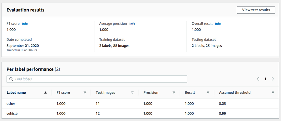
When Amazon Rekognition Custom Labels is finished training the model, you can view various evaluation metrics to determine how well the model is performing on the test set. The easiest way to view these metrics is to look on the console. The following screenshot shows the macro average metrics.
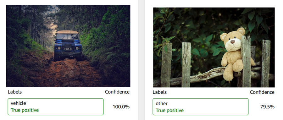
The following screenshot shows results for individual test images.
If you prefer to fetch these results programmatically, you first need to identify the output files that Amazon Rekognition Custom Labels has saved in the S3 bucket, so you can fetch the results stored in these files:
aws rekognition describe-project-versions
--project-arn <PROJECT_ARN>
--region us-west-2
Assuming the training process is complete, the output of this command provides the location of the output files. Amazon Rekognition Custom Labels saves the detailed results for each test image in a JSON file stored in Amazon S3. You can find the file details under TestingDataResult -> Output -> Assets -> GroundTruthManifest. The file name has the format TestingGroundTruth-<PROJECT_NAME>-<PROJECT_VERSION_NAME>.json. I recommend downloading this file to view it in an IDE, but you can also view the contents of the file without downloading it by using the following code (replace <S3_URI> with the URI of the file you want to view):
aws s3 cp <S3_URI> - | headSimilarly, Amazon Rekognition Custom Labels stores the macro average precision, recall, and F1 score in a JSON file, which you can find under EvaluationResults -> Summary. Again, you can view the contents of this file without downloading it by using the preceding command.
For this use case, the test set results in a precision and recall of 1, which means the model identified all the vehicle and non-vehicle images correctly. The assumed threshold used to generate the F1 score, precision, and recall metrics for vehicles is 0.99. By default, the model returns predictions above this assumed threshold. Examining the individual test images confirms that the model identifies vehicles with a consistently high confidence score. In addition to analyzing the test set results on the console, you can set up Custom Labels Demonstration UI to apply the model to images from your local computer.
Cleaning up
To avoid incurring future charges, clean up the following resources:
- Amazon Rekognition Custom Labels project
- Amazon SageMaker work team
- Amazon Cognito user pool
- S3 bucket
Conclusion
In this post, you learned how to create a labeled dataset and use it to train a custom computer vision model without any prior ML expertise. In addition, you learned how to accomplish all of this programmatically using the AWS CLI.
After gathering a collection of unlabeled images and storing these images in an S3 bucket, you set up a labeling job in Ground Truth and used the output of the labeling job to train a model in Amazon Rekognition Custom Labels. I hope you can apply this combination of AWS services to quickly create computer vision models for use cases in your own industry and domain.
To learn more, see the following resources:
- Use Amazon SageMaker Ground Truth to Label Data
- Amazon SageMaker Ground Truth: Using A Pre-Trained Model for Faster Data Labeling
- Amazon Rekognition Custom Labels Guide
- Amazon Rekognition Custom Labels Demo
About the Author
 Sara van de Moosdijk, simply known as Moose, is a Machine Learning Partner Solutions Architect at AWS Australia. She helps AWS partners build and scale AI/ML solutions through technical enablement, support, and architectural guidance. Moose spends her free time figuring out how to fit more books in her overflowing bookcase.
Alexa & Friends features Andrew Breen, Alexa TTS Research senior manager
Hear Breen discuss his work leading research teams in speech synthesis and text-to-speech technologies, the science behind Alexa’s enhanced voice styles, and more.Read More
Optimizing applications with EagleDream in Amazon CodeGuru Profiler
This is a guest post by Dustin Potter at EagleDream Technologies. In their own words, “EagleDream Technologies educates, enables, and empowers the world’s greatest companies to use cloud-native technology to transform their business. With extensive experience architecting workloads on the cloud, as well as a full suite of skills in application modernization, data engineering, data lake design, and analytics, EagleDream has built a growing practice in helping businesses redefine what’s possible with technology.”
EagleDream Technologies is a trusted cloud-native transformation company and APN Premier Consulting Partner for businesses using AWS. EagleDream is unique in using its cloud-native software engineering and application modernization expertise to guide you through your journey to the cloud, optimize your operations, and transform how you do business using AWS. Our team of highly trained professionals helps accelerate projects at every stage of the cloud journey. This post shares our experience using Amazon CodeGuru Profiler to help one of our customers optimize their application under tight deadlines.
Project overview
Our team received a unique opportunity to work with one of the industry’s most disruptive airline technology leaders, who uses their expertise to build custom integrated airline booking, loyalty management, and ecommerce platforms. This customer reached out to our team to help optimize their new application. They already had a few clients using the system, but they recently signed a deal with a major airline that would represent a load increase to their platform five times in size. It was critical that they prepare for this significant increase in activity. The customer was running a traditional three-tier application written in Java that used Amazon Aurora for the data layer. They had already implemented autoscaling for the web servers and database but realized something was wrong when they started running load tests. During the first load test, the web tier expanded to over 80 servers and Aurora reached the max number of read replicas.
Our team knew we had to dive deep and investigate the application code. We had previously used other application profiling tools and realized how invaluable they can be when diagnosing these types of issues. Also, AWS recently announced Amazon CodeGuru and we were eager to try it out. On top of that, the price and ease of setup was a driving factor for us. We had looked at an existing commercial application performance monitoring tool, but it required more invasive changes to utilize. To automate the install of these tools, we would have needed to make changes to the customer’s deployment and infrastructure setup. We had to move quickly with as little disruption to their ongoing feature development as possible, which contributed to our final decision to use CodeGuru.
CodeGuru workflow
After we decided on CodeGuru, it was easy to get CodeGuru Profiler installed and start capturing metrics. There are two ways to profile an application. The first is to reference the profiler agent during the start of the application by using the standard -javaagent parameter. This is useful if the group performing the profiling isn’t the development team, for example in an organization with more traditional development and operation silos. This is easy to set up because all that’s needed is to download the .jar published in the documentation and alter any startup scripts to include the agent and the name of the profiling group to use.
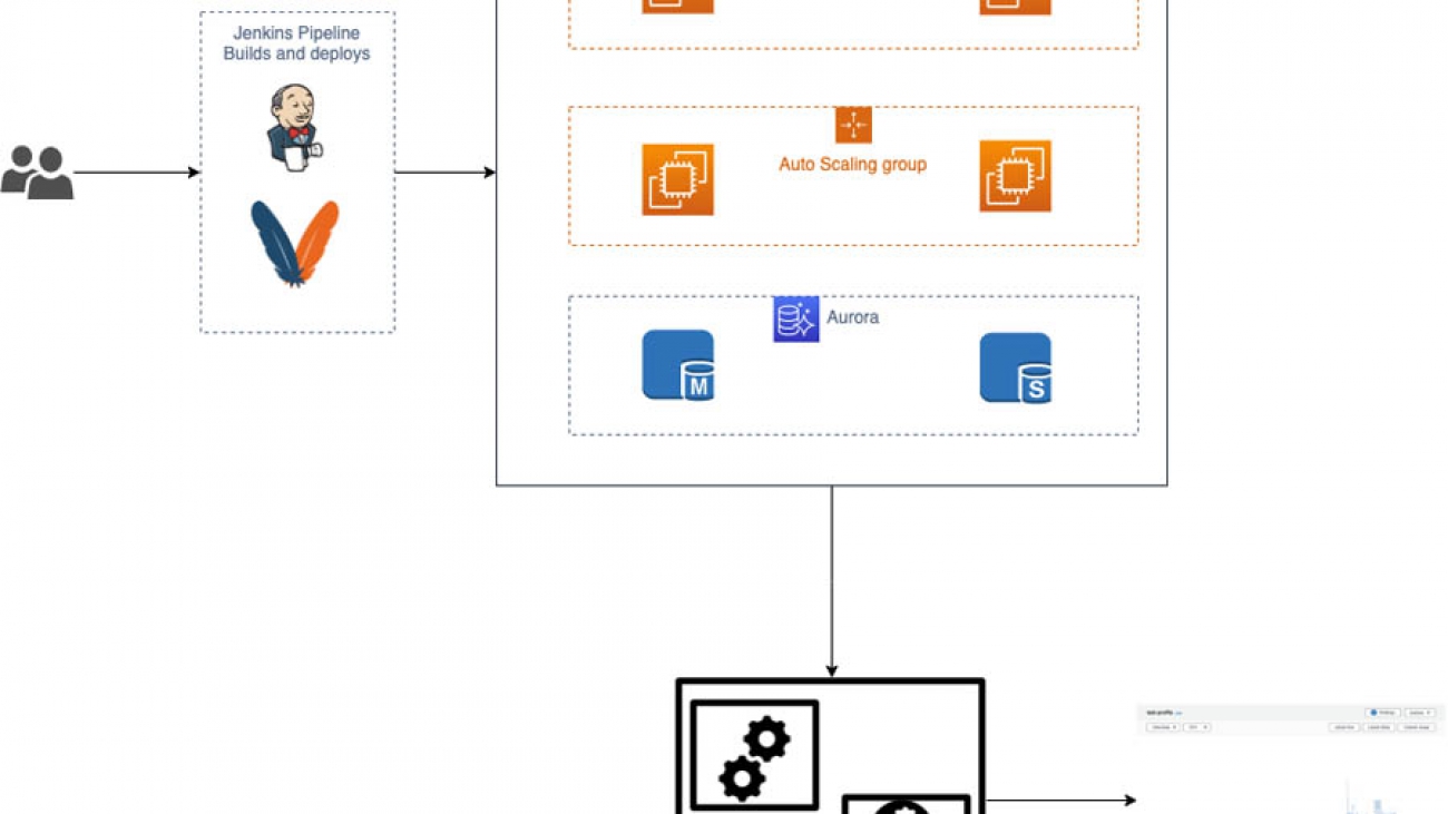
The second way to profile the application is to include the profiler code via a dependency in your build system and instantiate a profiling thread somewhere at the entry point of the program. This option is great if the development team is handling the profiling. For this particular use case, we fell into the second group, so including it in the code was the quickest and easiest approach. We added the library as a Maven dependency and added a single line of application code. After the code was committed, we used the customer’s existing Jenkins setup to deploy the latest build to an integration environment. The final step of the pipeline was to run load tests against the new build. After the tests completed, we had a flame graph that we used to start identifying any issues.
The workflow includes the following steps:
- Developers check in code.
- The check-in triggers a Jenkins job.
- Maven compiles the code.
- Jenkins deploys the artifact to the development environment.
- Load tests run against the newly deployed code.
- CodeGuru Profiler monitors the environment and generates a flame graph and a recommendation report.
The following diagram illustrates the workflow.

Flame graphs group together stack traces and highlight which part of the code consumes the most resources. The following screenshot is a sample flame graph from an AWS demo application for reference.

After CodeGuru generated the flame graphs and recommendations report, we took an iterative approach and tackled the biggest offenders first. The flame graphs provided perceptive guidance for actionable recommendations that it discovers and made it easy to identify which execution paths were taking the longest to complete. By looking at the longest frames first, we identified that the customer faced challenges around thread safety, which was leading to locking issues. To resolve issues collaboratively with the client, we created a Slack channel to review the latest graphs and provide recommendations directly to the developers. After the developers implemented the suggested changes, we deployed a new build and had a corresponding graph in a few minutes.
Results
After just one week, our team successfully alleviated their scaling challenges at the web service layer. When we ran the load tests, we saw expected results of a few servers instead of the more than 80 servers previously. Additionally, because we optimized the code, we reduced the existing application footprint, which saved our customer 30% of compute load.
Cost savings aside, one of the most notable benefits of this project was developer education. With CodeGuru Profiler pinpointing where the bottlenecks were, the developers could recognize inefficient patterns in the code that might lead to severe performance hits down the road. This helped them better understand the features of the language they’re using and armed them with increased efficiency in future development and debugging.
Conclusion
With the web service layer better optimized, our next step is to use CodeGuru and other AWS tools like Performance Insights to tackle the database layer. Even if you aren’t experiencing extreme performance challenges, CodeGuru Profiler can provide valuable insights to the health of your application in any environment, from development all the way to production, with minimal CPU utilization. Integrating these results as part of the SDLC or DevOps process leads to better efficiency and gives you and your developers the tools you need to be successful. To learn more about how to get started with CodeGuru Profiler and CodeGuru Reviewer, check the documentation found here.
About the Author
Dustin Potter is a Principal Cloud Solutions Architect at EagleDream Technologies.
Amazon Translate ranked as #1 machine translation provider by Intento
Customer obsession, one of the key Amazon Leadership principles that guides everything we do at Amazon, has helped Amazon Translate be recognized as an industry leading neural machine translation provider. This year, Intento ranked Amazon Translate #1 on the list of top-performing machine translation providers in its The State of Machine Translation 2020 report. We are excited to be recognized for pursuing our passion—designing the best customer experience in machine translation.
Amazon Translate is a neural machine translation service that delivers fast, high-quality, and affordable language translation. Neural machine translation is a form of machine translation that uses deep learning models to deliver more accurate and more natural sounding translation than traditional statistical and rule-based translation algorithms. Amazon Translate’s development has been fueled by customer feedback, leading to a steady stream of rich features that help you reach more people in more places—without breaking your translation services budget.
Intento is one of the leading organizations helping global companies procure and utilize the best-fit cognitive AI services. In this independent study, Intento evaluated 15 of the most prominent MT providers used by language service providers and localization services. The data used included examples from across 16 industry sectors, with 8 content types, including topics such as financial documentation, patents, sales and marketing material. These inputs were translated between 14 common language pairs to determine the best engine for a given translation scenario. It ranked the results of each MT engine based on how they compared to a reference human translation.
The results showed that no MT service is best in all language pairs across all industry sectors and content types. However, Amazon Translate had the highest number of instances in which it was rated “best.”
At Amazon, we strive to bring the most value to our customers and deliver the world’s best machine translation service! If your company is looking for machine translation, please contact us. We’d love to show you what Amazon Translate can do.
More information on the features and capabilities that Intento considered in its analysis of the top MT providers is available in the full report (registration is required).
About the Author
 Greg Rushing is a US Air Force Fellow in Amazon’s BRIDGE program. He is currently working with the Amazon Translate Product Management team, where he focuses on coordinating the activities required to bring Amazon Translate features to market. Outside of work, you can find him spending time exploring the outdoors with his family, doing auto repair, or woodworking.
Building a medical image search platform on AWS
Improving radiologist efficiency and preventing burnout is a primary goal for healthcare providers. A nationwide study published in Mayo Clinic Proceedings in 2015 showed radiologist burnout percentage at a concerning 61% [1]. In additon, the report concludes that “burnout and satisfaction with work-life balance in US physicians worsened from 2011 to 2014. More than half of US physicians are now experiencing professional burnout.”[2] As technologists, we’re looking for ways to put new and innovative solutions in the hands of physicians to make them more efficient, reduce burnout, and improve care quality.
To reduce burnout and improve value-based care through data-driven decision-making, Artificial Intelligence (AI) can be used to unlock the information trapped in the vast amount of unstructured data (e.g. images, texts, and voice) and create clinically actionable knowledge base. AWS AI services can derive insights and relationships from free-form medical reports, automate the knowledge sharing process, and eventually improve personalized care experience.
In this post, we use Convolutional Neural Networks (CNN) as a feature extractor to convert medical images into a one-dimensional feature vector with a size of 1024. We call this process medical image embedding. Then we index the image feature vector using the K-nearest neighbors (KNN) algorithm in Amazon Elasticsearch Service (Amazon ES) to build a similarity-based image retrieval system. Additionally, we use the AWS managed natural language processing (NLP) service Amazon Comprehend Medical to perform named entity recognition (NER) against free text clinical reports. The detected named entities are also linked to medical ontology, ICD-10-CM, to enable simple aggregation and distribution analysis. The presented solution also includes a front-end React web application and backend GraphQL API managed by AWS Amplify and AWS AppSync, and authentication is handled by Amazon Cognito.
After deploying this working solution, the end-users (healthcare providers) can search through a repository of unstructured free text and medical images, conduct analytical operations, and use it in medical training and clinical decision support. This eliminates the need to manually analyze all the images and reports and get to the most relevant ones. Using a system like this improves the provider’s efficiency. The following graphic shows an example end result of the deployed application.
Dataset and architecture
We use the MIMIC CXR dataset to demonstrate how this working solution can benefit healthcare providers, in particular, radiologists. MIMIC CXR is a publicly available database of chest X-ray images in DICOM format and the associated radiology reports as free text files[3]. The methods for data collection and the data structures in this dataset have been well documented and are very detailed [3]. Also, this is a restricted-access resource. To access the files, you must be a registered user and sign the data use agreement. The following sections provide more details on the components of the architecture.
The following diagram illustrates the solution architecture.

The architecture is comprised of the offline data transformation and online query components. The offline data transformation step, the unstructured data, including free texts and image files, is converted into structured data.
Electronic Heath Record (EHR) radiology reports as free text are processed using Amazon Comprehend Medical, an NLP service that uses machine learning to extract relevant medical information from unstructured text, such as medical conditions including clinical signs, diagnosis, and symptoms. The named entities are identified and mapped to structured vocabularies, such as ICD-10 Clinical Modifications (CMs) ontology. The unstructured text plus structured named entities are stored in Amazon ES to enable free text search and term aggregations.
The medical images from Picture Archiving and Communication System (PACS) are converted into vector representations using a pretrained deep learning model deployed in an Amazon Elastic Container Service (Amazon ECS) AWS Fargate cluster. Similar visual search on AWS has been published previously for online retail product image search. It used an Amazon SageMaker built-in KNN algorithm for similarity search, which supports different index types and distance metrics.
We took advantage of the KNN for Amazon ES to find the k closest images from a feature space as demonstrated on the GitHub repo. KNN search is supported in Amazon ES version 7.4+. The container running on the ECS Fargate cluster reads medical images in DICOM format, carries out image embedding using a pretrained model, and saves a PNG thumbnail in an Amazon Simple Storage Service (Amazon S3) bucket, which serves as the storage for AWS Amplify React web application. It also parses out the DICOM image metadata and saves them in Amazon DynamoDB. The image vectors are saved in an Elasticsearch cluster and are used for the KNN visual search, which is implemented in an AWS Lambda function.
The unstructured data from EHR and PACS needs to be transferred to Amazon S3 to trigger the serverless data processing pipeline through the Lambda functions. You can achieve this data transfer by using AWS Storage Gateway or AWS DataSync, which is out of the scope of this post. The online query API, including the GraphQL schemas and resolvers, was developed in AWS AppSync. The front-end web application was developed using the Amplify React framework, which can be deployed using the Amplify CLI. The detailed AWS CloudFormation templates and sample code are available in the Github repo.
Solution overview
To deploy the solution, you complete the following steps:
- Deploy the Amplify React web application for online search.
- Deploy the image-embedding container to AWS Fargate.
- Deploy the data-processing pipeline and AWS AppSync API.
Deploying the Amplify React web application
The first step creates the Amplify React web application, as shown in the following diagram.

- Install and configure the AWS Command Line Interface (AWS CLI).
- Install the AWS Amplify CLI.
- Clone the code base with stepwise instructions.
- Go to your code base folder and initialize the Amplify app using the command
amplify init. You must answer a series of questions, like the name of the Amplify app.
After this step, you have the following changes in your local and cloud environments:
- A new folder named
amplifyis created in your local environment - A file named
aws-exports.jsis created in local thesrcfolder - A new Amplify app is created on the AWS Cloud with the name provided during deployment (for example,
medical-image-search) - A CloudFormation stack is created on the AWS Cloud with the prefix
amplify-<AppName>
You create authentication and storage services for your Amplify app afterwards using the following commands:
amplify add auth
amplify add storage
amplify push
When the CloudFormation nested stacks for authentication and storage are successfully deployed, you can see the new Amazon Cognito user pool as the authentication backend and S3 bucket as the storage backend are created. Save the Amazon Cognito user pool ID and S3 bucket name from the Outputs tab of the corresponding CloudFormation nested stack (you use these later).
The following screenshot shows the location of the user pool ID on the Outputs tab.

The following screenshot shows the location of the bucket name on the Outputs tab.

Deploying the image-embedding container to AWS Fargate
We use the Amazon SageMaker Inference Toolkit to serve the PyTorch inference model, which converts a medical image in DICOM format into a feature vector with the size of 1024. To create a container with all the dependencies, you can either use pre-built deep learning container images or derive a Dockerfile from the Amazon Sagemaker Pytorch inference CPU container, like the one from the GitHub repo, in the container folder. You can build the Docker container and push it to Amazon ECR manually or by running the shell script build_and_push.sh. You use the repository image URI for the Docker container later to deploy the AWS Fargate cluster.
The following screenshot shows the sagemaker-pytorch-inference repository on the Amazon ECR console.

We use Multi Model Server (MMS) to serve the inference endpoint. You need to install MMS with pip locally, use the Model archiver CLI to package model artifacts into a single model archive .mar file, and upload it to an S3 bucket to be served by a containerized inference endpoint. The model inference handler is defined in dicom_featurization_service.py in the MMS folder. If you have a domain-specific pretrained Pytorch model, place the model.pth file in the MMS folder; otherwise, the handler uses a pretrained DenseNET121[4] for image processing. See the following code:
model_file_path = os.path.join(model_dir, "model.pth")
if os.path.isfile(model_file_path):
    model = torch.load(model_file_path)
else:
    model = models.densenet121(pretrained=True)
    model = model._modules.get('features')
    model.add_module("end_relu", nn.ReLU())
    model.add_module("end_globpool", nn.AdaptiveAvgPool2d((1, 1)))
    model.add_module("end_flatten", nn.Flatten())
model = model.to(self.device)
model.eval()
The intermediate results of this CNN-based model is to represent images as feature vectors. In other words, the convolutional layers before the final classification layer is flattened to convert feature layers to a vector representation. Run the following command in the MMS folder to package up the model archive file:
model-archiver -f --model-name dicom_featurization_service --model-path ./ --handler dicom_featurization_service:handle --export-path ./The preceding code generates a package file named dicom_featurization_service.mar. Create a new S3 bucket and upload the package file to that bucket with public read Access Control List (ACL). See the following code:
aws s3 cp ./dicom_featurization_service.mar s3://<S3bucketname>/ --acl public-read --profile <profilename>You’re now ready to deploy the image-embedding inference model to the AWS Fargate cluster using the CloudFormation template ecsfargate.yaml in the CloudFormationTemplates folder. You can deploy using the AWS CLI: go to the CloudFormationTemplates folder and copy the following command:
aws cloudformation deploy --capabilities CAPABILITY_IAM --template-file ./ecsfargate.yaml --stack-name <stackname> --parameter-overrides ImageUrl=<imageURI> InferenceModelS3Location=https://<S3bucketname>.s3.amazonaws.com/dicom_featurization_service.mar --profile <profilename>You need to replace the following placeholders:
- stackname – A unique name to refer to this CloudFormation stack
- imageURI – The image URI for the MMS Docker container uploaded in Amazon ECR
- S3bucketname – The MMS package in the S3 bucket, such as
https://<S3bucketname>.s3.amazonaws.com/dicom_featurization_service.mar - profilename – Your AWS CLI profile name (default if not named)
Alternatively, you can choose Launch stack for the following Regions:
- us-east-1 –
- us-west-2 –
After the CloudFormation stack creation is complete, go to the stack Outputs tab on the AWS CloudFormation console and copy the InferenceAPIUrl for later deployment. See the following screenshot.

You can delete this stack after the offline image embedding jobs are finished to save costs, because it’s not used for online queries.
Deploying the data-processing pipeline and AWS AppSync API
You deploy the image and free text data-processing pipeline and AWS AppSync API backend through another CloudFormation template named AppSyncBackend.yaml in the CloudFormationTemplates folder, which creates the AWS resources for this solution. See the following solution architecture.

To deploy this stack using the AWS CLI, go to the CloudFormationTemplates folder and copy the following command:
aws cloudformation deploy --capabilities CAPABILITY_NAMED_IAM --template-file ./AppSyncBackend.yaml --stack-name <stackname> --parameter-overrides AuthorizationUserPool=<CFN_output_auth> PNGBucketName=<CFN_output_storage> InferenceEndpointURL=<inferenceAPIUrl> --profile <profilename>Replace the following placeholders:
- stackname – A unique name to refer to this CloudFormation stack
- AuthorizationUserPool – Amazon Cognito user pool
- PNGBucketName – Amazon S3 bucket name
- InferenceEndpointURL – The inference API endpoint
- Profilename – The AWS CLI profile name (use default if not named)
Alternatively, you can choose Launch stack for the following Regions:
- us-east-1 –
- us-west-2 –
You can download the Lambda function for medical image processing, CMprocessLambdaFunction.py, and its dependency layer separately if you deploy this stack in AWS Regions other than us-east-1 and us-west-2. Because their file size exceeds the CloudFormation template limit, you need to upload them to your own S3 bucket (either create a new S3 bucket or use the existing one, like the aforementioned S3 bucket for hosting the MMS model package file) and override the LambdaBucket mapping parameter using your own bucket name.
Save the AWS AppySync API URL and AWS Region from the settings on the AWS AppSync console.

Edit the src/aws-exports.js file in your local environment and replace the placeholders with those values:
const awsmobile = {
  "aws_appsync_graphqlEndpoint": "<AppSync API URL>",
  "aws_appsync_region": "<AWS AppSync Region>",
  "aws_appsync_authenticationType": "AMAZON_COGNITO_USER_POOLS"
};
After this stack is successfully deployed, you’re ready to use this solution. If you have in-house EHR and PACS databases, you can set up the AWS Storage Gateway to transfer data to the S3 bucket to trigger the transformation jobs.
Alternatively, you can use the public dataset MIMIC CXR: download the MIMIC CXR dataset from PhysioNet (to access the files, you must be a credentialed user and sign the data use agreement for the project) and upload the DICOM files to the S3 bucket mimic-cxr-dicom- and the free text radiology report to the S3 bucket mimic-cxr-report-. If everything works as expected, you should see the new records created in the DynamoDB table medical-image-metadata and the Amazon ES domain medical-image-search.
You can test the Amplify React web application locally by running the following command:
npm install && npm startOr you can publish the React web app by deploying it in Amazon S3 with AWS CloudFront distribution, by first entering the following code:
amplify hosting addThen, enter the following code:
amplify publishYou can see the hosting endpoint for the Amplify React web application after deployment.
Conclusion
We have demonstrated how to deploy, index and search medical images on AWS, which segregates the offline data ingestion and online search query functions. You can use AWS AI services to transform unstructured data, for example the medical images and radiology reports, into structured ones.
By default, the solution uses a general-purpose model trained on ImageNET to extract features from images. However, this default model may not be accurate enough to extract medical image features because there are fundamental differences in appearance, size, and features between medical images in its raw form. Such differences make it hard to train commonly adopted triplet-based learning networks [5], where semantically relevant images or objects can be easily defined or ranked.
To improve search relevancy, we performed an experiment by using the same MIMIC CXR dataset and the derived diagnosis labels to train a weakly supervised disease classification network similar to Wang et. Al [6]. We found this domain-specific pretrained model yielded qualitatively better visual search results. So it’s recommended to bring your own model (BYOM) to this search platform for real-world implementation.
The methods presented here enable you to perform indexing, searching and aggregation against unstructured images in addition to free text. It sets the stage for future work that can combine these features for multimodal medical image search engine. Information retrieval from unstructured corpuses of clinical notes and images is a time-consuming and tedious task. Our solution allows radiologists to become more efficient and help them reduce potential burnout.
To find the latest development to this solution, check out medical image search on GitHub.
Reference:
- https://www.radiologybusiness.com/topics/leadership/radiologist-burnout-are-we-done-yet
- https://www.mayoclinicproceedings.org/article/S0025-6196(15)00716-8/abstract#secsectitle0010
- Johnson, Alistair EW, et al. “MIMIC-CXR, a de-identified publicly available database of chest radiographs with free-text reports.” Scientific Data 6, 2019.
- Huang, Gao, et al. “Densely connected convolutional networks.” Proceedings of the IEEE Conference on Computer Vision and Pattern Recognition, 2017.
- Wang, Jiang, et al. “Learning fine-grained image similarity with deep ranking.” Proceedings of the IEEE Conference on Computer Vision and Pattern Recognition, 2014.
- Wang, Xiaosong, et al. “Chestx-ray8: Hospital-scale chest x-ray database and benchmarks on weakly-supervised classification and localization of common thorax diseases.” Proceedings of the IEEE Conference on Computer Vision and Pattern Recognition, 2017.
About the Authors
 Gang Fu is a Healthcare Solution Architect at AWS. He holds a PhD in Pharmaceutical Science from the University of Mississippi and has over ten years of technology and biomedical research experience. He is passionate about technology and the impact it can make on healthcare.
 Ujjwal Ratan is a Principal Machine Learning Specialist Solution Architect in the Global Healthcare and Lifesciences team at Amazon Web Services. He works on the application of machine learning and deep learning to real world industry problems like medical imaging, unstructured clinical text, genomics, precision medicine, clinical trials and quality of care improvement. He has expertise in scaling machine learning/deep learning algorithms on the AWS cloud for accelerated training and inference. In his free time, he enjoys listening to (and playing) music and taking unplanned road trips with his family.
 Erhan Bas is a Senior Applied Scientist in the AWS Rekognition team, currently developing deep learning algorithms for computer vision applications. His expertise is in machine learning and large scale image analysis techniques, especially in biomedical, life sciences and industrial inspection technologies. He enjoys playing video games, drinking coffee, and traveling with his family.
Streamlining data labeling for YOLO object detection in Amazon SageMaker Ground Truth
Object detection is a common task in computer vision (CV), and the YOLOv3 model is state-of-the-art in terms of accuracy and speed. In transfer learning, you obtain a model trained on a large but generic dataset and retrain the model on your custom dataset. One of the most time-consuming parts in transfer learning is collecting and labeling image data to generate a custom training dataset. This post explores how to do this in Amazon SageMaker Ground Truth.
Ground Truth offers a comprehensive platform for annotating the most common data labeling jobs in CV: image classification, object detection, semantic segmentation, and instance segmentation. You can perform labeling using Amazon Mechanical Turk or create your own private team to label collaboratively. You can also use one of the third-party data labeling service providers listed on the AWS Marketplace. Ground Truth offers an intuitive interface that is easy to work with. You can communicate with labelers about specific needs for your particular task using examples and notes through the interface.
Labeling data is already hard work. Creating training data for a CV modeling task requires data collection and storage, setting up labeling jobs, and post-processing the labeled data. Moreover, not all object detection models expect the data in the same format. For example, the Faster RCNN model expects the data in the popular Pascal VOC format, which the YOLO models can’t work with. These associated steps are part of any machine learning pipeline for CV. You sometimes need to run the pipeline multiple times to improve the model incrementally. This post shows how to perform these steps efficiently by using Python scripts and get to model training as quickly as possible. This post uses the YOLO format for its use case, but the steps are mostly independent of the data format.
The image labeling step of a training data generation task is inherently manual. This post shows how to create a reusable framework to create training data for model building efficiently. Specifically, you can do the following:
- Create the required directory structure in Amazon S3 before starting a Ground Truth job
- Create a private team of annotators and start a Ground Truth job
- Collect the annotations when labeling is complete and save it in a pandas dataframe
- Post-process the dataset for model training
You can download the code presented in this post from this GitHub repo. This post demonstrates how to run the code from the AWS CLI on a local machine that can access an AWS account. For more information about setting up AWS CLI, see What Is the AWS Command Line Interface? Make sure that you configure it to access the S3 buckets in this post. Alternatively, you can run it in AWS Cloud9 or by spinning up an Amazon EC2 instance. You can also run the code blocks in an Amazon SageMaker notebook.
If you’re using an Amazon SageMaker notebook, you can still access the Linux shell of the underlying EC2 instance and follow along by opening a new terminal from the Jupyter main page and running the scripts from the /home/ec2-user/SageMaker folder.
Setting up your S3 bucket
The first thing you need to do is to upload the training images to an S3 bucket. Name the bucket ground-truth-data-labeling. You want each labeling task to have its own self-contained folder under this bucket. If you start labeling a small set of images that you keep in the first folder, but find that the model performed poorly after the first round because the data was insufficient, you can upload more images to a different folder under the same bucket and start another labeling task.
For the first labeling task, create the folder bounding_box and the following three subfolders under it:
- images – You upload all the images in the Ground Truth labeling job to this subfolder.
- ground_truth_annots – This subfolder starts empty; the Ground Truth job populates it automatically, and you retrieve the final annotations from here.
- yolo_annot_files – This subfolder also starts empty, but eventually holds the annotation files ready for model training. The script populates it automatically.
If your images are in .jpeg format and available in the current working directory, you can upload the images with the following code:
aws s3 sync . s3://ground-truth-data-labeling/bounding_box/images/ --exclude "*" --include "*.jpg" For this use case, you use five images. There are two types of objects in the images—pencil and pen. You need to draw bounding boxes around each object in the images. The following images are examples of what you need to label. All images are available in the GitHub repo.


Creating the manifest file
A Ground Truth job requires a manifest file in JSON format that contains the Amazon S3 paths of all the images to label. You need to create this file before you can start the first Ground Truth job. The format of this file is simple:
{"source-ref": < S3 path to image1 >}
{"source-ref": < S3 path to image2 >}
...
However, creating the manifest file by hand would be tedious for a large number of images. Therefore, you can automate the process by running a script. You first need to create a file holding the parameters required for the scripts. Create a file input.json in your local file system with the following content:
{
    "s3_bucket":"ground-truth-data-labeling",
    "job_id":"bounding_box",
    "ground_truth_job_name":"yolo-bbox",
    "yolo_output_dir":"yolo_annot_files"
}
Save the following code block in a file called prep_gt_job.py:
import boto3
import json


def create_manifest(job_path):
    """
    Creates the manifest file for the Ground Truth job

    Input:
    job_path: Full path of the folder in S3 for GT job

    Returns:
    manifest_file: The manifest file required for GT job
    """

    s3_rec = boto3.resource("s3")
    s3_bucket = job_path.split("/")[0]
    prefix = job_path.replace(s3_bucket, "")[1:]
    image_folder = f"{prefix}/images"
    print(f"using images from ... {image_folder} n")

    bucket = s3_rec.Bucket(s3_bucket)
    objs = list(bucket.objects.filter(Prefix=image_folder))
    img_files = objs[1:]  # first item is the folder name
    n_imgs = len(img_files)
    print(f"there are {n_imgs} images n")

    TOKEN = "source-ref"
    manifest_file = "/tmp/manifest.json"
    with open(manifest_file, "w") as fout:
        for img_file in img_files:
            fname = f"s3://{s3_bucket}/{img_file.key}"
            fout.write(f'{{"{TOKEN}": "{fname}"}}n')

    return manifest_file


def upload_manifest(job_path, manifest_file):
    """
    Uploads the manifest file into S3

    Input:
    job_path: Full path of the folder in S3 for GT job
    manifest_file: Path to the local copy of the manifest file
    """

    s3_rec = boto3.resource("s3")
    s3_bucket = job_path.split("/")[0]
    source = manifest_file.split("/")[-1]
    prefix = job_path.replace(s3_bucket, "")[1:]
    destination = f"{prefix}/{source}"

    print(f"uploading manifest file to {destination} n")
    s3_rec.meta.client.upload_file(manifest_file, s3_bucket, destination)


def main():
    """
    Performs the following tasks:
    1. Reads input from 'input.json'
    2. Collects image names from S3 and creates the manifest file for GT
    3. Uploads the manifest file to S3
    """

    with open("input.json") as fjson:
        input_dict = json.load(fjson)

    s3_bucket = input_dict["s3_bucket"]
    job_id = input_dict["job_id"]

    gt_job_path = f"{s3_bucket}/{job_id}"
    man_file = create_manifest(gt_job_path)
    upload_manifest(gt_job_path, man_file)


if __name__ == "__main__":
    main()
Run the following script:
python prep_gt_job.py
This script reads the S3 bucket and job names from the input file, creates a list of images available in the images folder, creates the manifest.json file, and uploads the manifest file to the S3 bucket at s3://ground-truth-data-labeling/bounding_box/.
This method illustrates a programmatic control of the process, but you can also create the file from the Ground Truth API. For instructions, see Create a Manifest File.
At this point, the folder structure in the S3 bucket should look like the following:
ground-truth-data-labeling
|-- bounding_box
    |-- ground_truth_annots
    |-- images
    |-- yolo_annot_files
    |-- manifest.json
Creating the Ground Truth job
You’re now ready to create your Ground Truth job. You need to specify the job details and task type, and create your team of labelers and labeling task details. Then you can sign in to begin the labeling job.
Specifying the job details
To specify the job details, complete the following steps:
- On the Amazon SageMaker console, under Ground Truth, choose Labeling jobs.
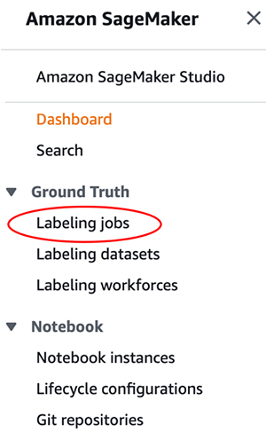
- On the Labeling jobs page, choose Create labeling job.

- In the Job overview section, for Job name, enter
yolo-bbox. It should be the name you defined in theinput.jsonfile earlier. - Pick Manual Data Setup under Input Data Setup.
- For Input dataset location, enter
s3://ground-truth-data-labeling/bounding_box/manifest.json. - For Output dataset location, enter
s3://ground-truth-data-labeling/bounding_box/ground_truth_annots.
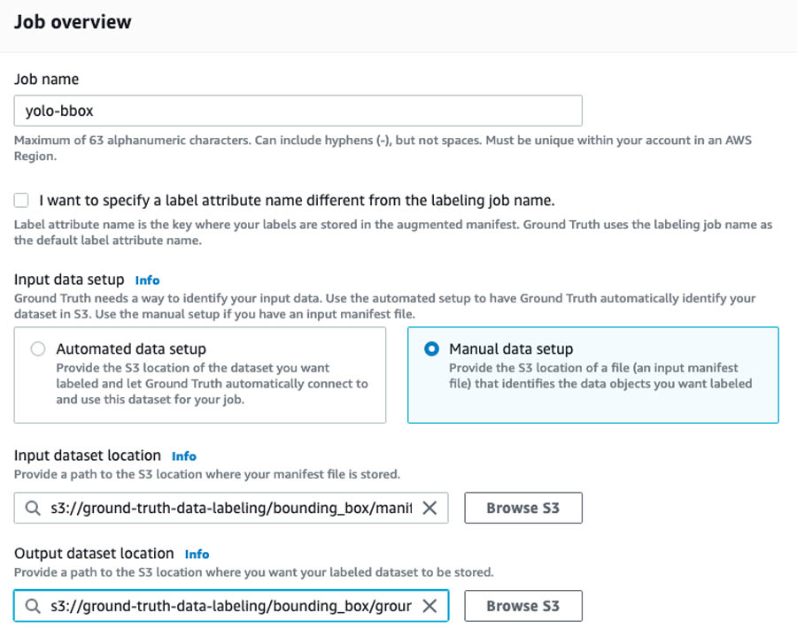
- In the Create an IAM role section, first select Create a new role from the drop down menu and then select Specific S3 buckets.
- Enter ground-truth-data-labeling.
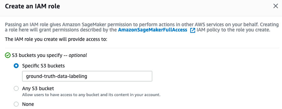
- Choose Create.
Specifying the task type
To specify the task type, complete the following steps:
- In the Task selection section, from the Task Category drop-down menu, choose Image.
- Select Bounding box.
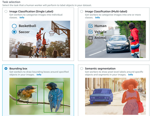
- Don’t change Enable enhanced image access, which is selected by default. It enables Cross-Origin Resource Sharing (CORS) that may be required for some workers to complete the annotation task.
- Choose Next.
Creating a team of labelers
To create your team of labelers, complete the following steps:
- In the Workers section, select Private.
- Follow the instructions to create a new team.

Each member of the team receives a notification email titled, “You’re invited to work on a labeling project” that has initial sign-in credentials. For this use case, create a team with just yourself as a member.
Specifying labeling task details
In the Bounding box labeling tool section, you should see the images you uploaded to Amazon S3. You should check that the paths are correct in the previous steps. To specify your task details, complete the following steps:
- In the text box, enter a brief description of the task.
This is critical if the data labeling team has more than one members and you want to make sure everyone follows the same rule when drawing the boxes. Any inconsistency in bounding box creation may end up confusing your object detection model. For example, if you’re labeling beverage cans and want to create a tight bounding box only around the visible logo, instead of the entire can, you should specify that to get consistent labeling from all the workers. For this use case, you can enter Please enter a tight bounding box around the entire object.
- Optionally, you can upload examples of a good and a bad bounding box.
You can make sure your team is consistent in their labels by providing good and bad examples.
- Under Labels, enter the names of the labels you’re using to identify each bounding box; in this case,
pencilandpen.
A color is assigned to each label automatically, which helps to visualize the boxes created for overlapping objects.
- To run a final sanity check, choose Preview.
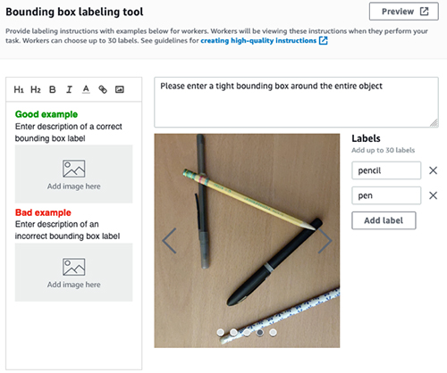
- Choose Create job.
Job creation can take up to a few minutes. When it’s complete, you should see a job titled yolo-bbox on the Ground Truth Labeling jobs page with In progress as the status.
- To view the job details, select the job.
This is a good time to verify the paths are correct; the scripts don’t run if there’s any inconsistency in names.
For more information about providing labeling instructions, see Create high-quality instructions for Amazon SageMaker Ground Truth labeling jobs.
Sign in and start labeling
After you receive the initial credentials to register as a labeler for this job, follow the link to reset the password and start labeling.
If you need to interrupt your labeling session, you can resume labeling by choosing Labeling workforces under Ground Truth on the SageMaker console.
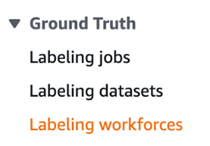
You can find the link to the labeling portal on the Private tab. The page also lists the teams and individuals involved in this private labeling task.
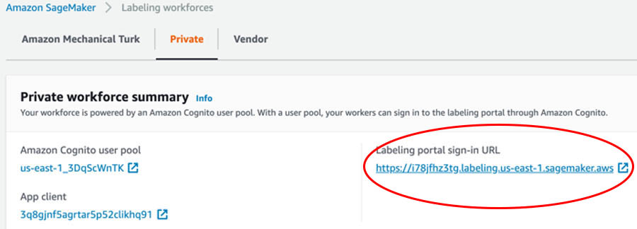
After you sign in, start labeling by choosing Start working.

Because you only have five images in the dataset to label, you can finish the entire task in a single session. For larger datasets, you can pause the task by choosing Stop working and return to the task later to finish it.
Checking job status
After the labeling is complete, the status of the labeling job changes to Complete and a new JSON file called output.manifest containing the annotations appears at s3://ground-truth-data-labeling/bounding_box/ground_truth_annots/yolo-bbox/manifests/output /output.manifest.
Parsing Ground Truth annotations
You can now parse through the annotations and perform the necessary post-processing steps to make it ready for model training. Start by running the following code block:
from io import StringIO
import json
import s3fs
import boto3
import pandas as pd


def parse_gt_output(manifest_path, job_name):
    """
    Captures the json Ground Truth bounding box annotations into a pandas dataframe

    Input:
    manifest_path: S3 path to the annotation file
    job_name: name of the Ground Truth job

    Returns:
    df_bbox: pandas dataframe with bounding box coordinates
             for each item in every image
    """

    filesys = s3fs.S3FileSystem()
    with filesys.open(manifest_path) as fin:
        annot_list = []
        for line in fin.readlines():
            record = json.loads(line)
            if job_name in record.keys():  # is it necessary?
                image_file_path = record["source-ref"]
                image_file_name = image_file_path.split("/")[-1]
                class_maps = record[f"{job_name}-metadata"]["class-map"]

                imsize_list = record[job_name]["image_size"]
                assert len(imsize_list) == 1
                image_width = imsize_list[0]["width"]
                image_height = imsize_list[0]["height"]

                for annot in record[job_name]["annotations"]:
                    left = annot["left"]
                    top = annot["top"]
                    height = annot["height"]
                    width = annot["width"]
                    class_name = class_maps[f'{annot["class_id"]}']

                    annot_list.append(
                        [
                            image_file_name,
                            class_name,
                            left,
                            top,
                            height,
                            width,
                            image_width,
                            image_height,
                        ]
                    )

        df_bbox = pd.DataFrame(
            annot_list,
            columns=[
                "img_file",
                "category",
                "box_left",
                "box_top",
                "box_height",
                "box_width",
                "img_width",
                "img_height",
            ],
        )

    return df_bbox


def save_df_to_s3(df_local, s3_bucket, destination):
    """
    Saves a pandas dataframe to S3

    Input:
    df_local: Dataframe to save
    s3_bucket: Bucket name
    destination: Prefix
    """

    csv_buffer = StringIO()
    s3_resource = boto3.resource("s3")

    df_local.to_csv(csv_buffer, index=False)
    s3_resource.Object(s3_bucket, destination).put(Body=csv_buffer.getvalue())


def main():
    """
    Performs the following tasks:
    1. Reads input from 'input.json'
    2. Parses the Ground Truth annotations and creates a dataframe
    3. Saves the dataframe to S3
    """

    with open("input.json") as fjson:
        input_dict = json.load(fjson)

    s3_bucket = input_dict["s3_bucket"]
    job_id = input_dict["job_id"]
    gt_job_name = input_dict["ground_truth_job_name"]

    mani_path = f"s3://{s3_bucket}/{job_id}/ground_truth_annots/{gt_job_name}/manifests/output/output.manifest"

    df_annot = parse_gt_output(mani_path, gt_job_name)
    dest = f"{job_id}/ground_truth_annots/{gt_job_name}/annot.csv"
    save_df_to_s3(df_annot, s3_bucket, dest)


if __name__ == "__main__":
    main()
From the AWS CLI, save the preceding code block in the file parse_annot.py and run:
python parse_annot.py
Ground Truth returns the bounding box information using the following four numbers: x and y coordinates, and its height and width. The procedure parse_gt_output scans through the output.manifest file and stores the information for every bounding box for each image in a pandas dataframe. The procedure save_df_to_s3 saves it in a tabular format as annot.csv to the S3 bucket for further processing.
The creation of the dataframe is useful for a few reasons. JSON files are hard to read and the output.manifest file contains more information, like label metadata, than you need for the next step. The dataframe contains only the relevant information and you can visualize it easily to make sure everything looks fine.
To grab the annot.csv file from Amazon S3 and save a local copy, run the following:
aws s3 cp s3://ground-truth-data-labeling/bounding_box/ground_truth_annots/yolo-bbox/annot.csv You can read it back into a pandas dataframe and inspect the first few lines. See the following code:
import pandas as pd
df_ann = pd.read_csv('annot.csv')
df_ann.head()
The following screenshot shows the results.

You also capture the size of the image through img_width and img_height. This is necessary because the object detection models need to know the location of each bounding box within the image. In this case, you can see that images in the dataset were captured with a 4608×3456 pixel resolution.
There are quite a few reasons why it is a good idea to save the annotation information into a dataframe:
- In a subsequent step, you need to rescale the bounding box coordinates into a YOLO-readable format. You can do this operation easily in a dataframe.
- If you decide to capture and label more images in the future to augment the existing dataset, all you need to do is join the newly created dataframe with the existing one. Again, you can perform this easily using a dataframe.
- As of this writing, Ground Truth doesn’t allow through the console more than 30 different categories to label in the same job. If you have more categories in your dataset, you have to label them under multiple Ground Truth jobs and combine them. Ground Truth associates each bounding box to an integer index in the
output.manifestfile. Therefore, the integer labels are different across multiple Ground Truth jobs if you have more than 30 categories. Having the annotations as dataframes makes the task of combining them easier and takes care of the conflict of category names across multiple jobs. In the preceding screenshot, you can see that you used the actual names under the category column instead of the integer index.
Generating YOLO annotations
You’re now ready to reformat the bounding box coordinates Ground Truth provided into a format the YOLO model accepts.
In the YOLO format, each bounding box is described by the center coordinates of the box and its width and height. Each number is scaled by the dimensions of the image; therefore, they all range between 0 and 1. Instead of category names, YOLO models expect the corresponding integer categories.
Therefore, you need to map each name in the category column of the dataframe into a unique integer. Moreover, the official Darknet implementation of YOLOv3 needs to have the name of the image match the annotation text file name. For example, if the image file is pic01.jpg, the corresponding annotation file should be named pic01.txt.
The following code block performs all these tasks:
import os
import json
from io import StringIO
import boto3
import s3fs
import pandas as pd


def annot_yolo(annot_file, cats):
    """
    Prepares the annotation in YOLO format

    Input:
    annot_file: csv file containing Ground Truth annotations
    ordered_cats: List of object categories in proper order for model training

    Returns:
    df_ann: pandas dataframe with the following columns
            img_file int_category box_center_w box_center_h box_width box_height


    Note:
    YOLO data format: <object-class> <x_center> <y_center> <width> <height>
    """

    df_ann = pd.read_csv(annot_file)

    df_ann["int_category"] = df_ann["category"].apply(lambda x: cats.index(x))
    df_ann["box_center_w"] = df_ann["box_left"] + df_ann["box_width"] / 2
    df_ann["box_center_h"] = df_ann["box_top"] + df_ann["box_height"] / 2

    # scale box dimensions by image dimensions
    df_ann["box_center_w"] = df_ann["box_center_w"] / df_ann["img_width"]
    df_ann["box_center_h"] = df_ann["box_center_h"] / df_ann["img_height"]
    df_ann["box_width"] = df_ann["box_width"] / df_ann["img_width"]
    df_ann["box_height"] = df_ann["box_height"] / df_ann["img_height"]

    return df_ann


def save_annots_to_s3(s3_bucket, prefix, df_local):
    """
    For every image in the dataset, save a text file with annotation in YOLO format

    Input:
    s3_bucket: S3 bucket name
    prefix: Folder name under s3_bucket where files will be written
    df_local: pandas dataframe with the following columns
              img_file int_category box_center_w box_center_h box_width box_height
    """

    unique_images = df_local["img_file"].unique()
    s3_resource = boto3.resource("s3")

    for image_file in unique_images:
        df_single_img_annots = df_local.loc[df_local.img_file == image_file]
        annot_txt_file = image_file.split(".")[0] + ".txt"
        destination = f"{prefix}/{annot_txt_file}"

        csv_buffer = StringIO()
        df_single_img_annots.to_csv(
            csv_buffer,
            index=False,
            header=False,
            sep=" ",
            float_format="%.4f",
            columns=[
                "int_category",
                "box_center_w",
                "box_center_h",
                "box_width",
                "box_height",
            ],
        )
        s3_resource.Object(s3_bucket, destination).put(Body=csv_buffer.getvalue())


def get_cats(json_file):
    """
    Makes a list of the category names in proper order

    Input:
    json_file: s3 path of the json file containing the category information

    Returns:
    cats: List of category names
    """

    filesys = s3fs.S3FileSystem()
    with filesys.open(json_file) as fin:
        line = fin.readline()
        record = json.loads(line)
        labels = [item["label"] for item in record["labels"]]

    return labels


def main():
    """
    Performs the following tasks:
    1. Reads input from 'input.json'
    2. Collect the category names from the Ground Truth job
    3. Creates a dataframe with annotaion in YOLO format
    4. Saves a text file in S3 with YOLO annotations
       for each of the labeled images
    """

    with open("input.json") as fjson:
        input_dict = json.load(fjson)

    s3_bucket = input_dict["s3_bucket"]
    job_id = input_dict["job_id"]
    gt_job_name = input_dict["ground_truth_job_name"]
    yolo_output = input_dict["yolo_output_dir"]

    s3_path_cats = (
        f"s3://{s3_bucket}/{job_id}/ground_truth_annots/{gt_job_name}/annotation-tool/data.json"
    )
    categories = get_cats(s3_path_cats)
    print("n labels used in Ground Truth job: ")
    print(categories, "n")

    gt_annot_file = "annot.csv"
    s3_dir = f"{job_id}/{yolo_output}"
    print(f"annotation files saved in = ", s3_dir)

    df_annot = annot_yolo(gt_annot_file, categories)
    save_annots_to_s3(s3_bucket, s3_dir, df_annot)


if __name__ == "__main__":
    main()
From the AWS CLI, save the preceding code block in a file create_annot.py and run:
python create_annot.py
The annot_yolo procedure transforms the dataframe you created by rescaling the box coordinates by the image size, and the save_annots_to_s3 procedure saves the annotations corresponding to each image into a text file and stores it in Amazon S3.
You can now inspect a couple of images and their corresponding annotations to make sure they’re properly formatted for model training. However, you first need to write a procedure to draw YOLO formatted bounding boxes on an image. Save the following code block in visualize.py:
import matplotlib.pyplot as plt
import matplotlib.image as mpimg
import matplotlib.colors as mcolors
import argparse


def visualize_bbox(img_file, yolo_ann_file, label_dict, figure_size=(6, 8)):
    """
    Plots bounding boxes on images

    Input:
    img_file : numpy.array
    yolo_ann_file: Text file containing annotations in YOLO format
    label_dict: Dictionary of image categories
    figure_size: Figure size
    """

    img = mpimg.imread(img_file)
    fig, ax = plt.subplots(1, 1, figsize=figure_size)
    ax.imshow(img)

    im_height, im_width, _ = img.shape

    palette = mcolors.TABLEAU_COLORS
    colors = [c for c in palette.keys()]
    with open(yolo_ann_file, "r") as fin:
        for line in fin:
            cat, center_w, center_h, width, height = line.split()
            cat = int(cat)
            category_name = label_dict[cat]
            left = (float(center_w) - float(width) / 2) * im_width
            top = (float(center_h) - float(height) / 2) * im_height
            width = float(width) * im_width
            height = float(height) * im_height

            rect = plt.Rectangle(
                (left, top),
                width,
                height,
                fill=False,
                linewidth=2,
                edgecolor=colors[cat],
            )
            ax.add_patch(rect)
            props = dict(boxstyle="round", facecolor=colors[cat], alpha=0.5)
            ax.text(
                left,
                top,
                category_name,
                fontsize=14,
                verticalalignment="top",
                bbox=props,
            )
    plt.show()


def main():
    """
    Plots bounding boxes
    """

    labels = {0: "pen", 1: "pencil"}
    parser = argparse.ArgumentParser()
    parser.add_argument("img", help="image file")
    args = parser.parse_args()
    img_file = args.img
    ann_file = img_file.split(".")[0] + ".txt"
    visualize_bbox(img_file, ann_file, labels, figure_size=(6, 8))


if __name__ == "__main__":
    main()
Download an image and the corresponding annotation file from Amazon S3. See the following code:
aws s3 cp s3://ground-truth-data-labeling/bounding_box/yolo_annot_files/IMG_20200816_205004.txt .aws s3 cp s3://ground-truth-data-
labeling/bounding_box/images/IMG_20200816_205004.jpg .
To display the correct label of each bounding box, you need to specify the names of the objects you labeled in a dictionary and pass it to visualize_bbox. For this use case, you only have two items in the list. However, the order of the labels is important—it should match the order you used while creating the Ground Truth labeling job. If you can’t remember the order, you can access the information from the s3://data-labeling-ground-truth/bounding_box/ground_truth_annots/bbox-yolo/annotation-tool/data.json
file in Amazon S3, which the Ground Truth job creates automatically.
The contents of the data.json file the task look like the following code:
{"document-version":"2018-11-28","labels":[{"label":"pencil"},{"label":"pen"}]}Therefore, a dictionary with the labels as follows was created in visualize.py:
labels = {0: 'pencil', 1: 'pen'}Now run the following to visualize the image:
python visualize.py IMG_20200816_205004.jpgThe following screenshot shows the bounding boxes correctly drawn around two pens.
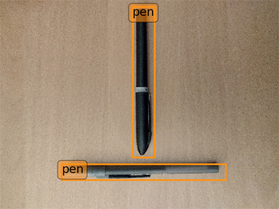
To plot an image with a mix of pens and pencils, get the image and the corresponding annotation text from Amazon S3. See the following code:
aws s3 cp s3://ground-truth-data-labeling/bounding_box/yolo_annot_files/IMG_20200816_205029.txt .

aws s3 cp s3://ground-truth-data-
labeling/bounding_box/images/IMG_20200816_205029.jpg .
Override the default image size in the visualize_bbox procedure to (10, 12) and run the following:
python visualize.py IMG_20200816_205029.jpgThe following screenshot shows three bounding boxes correctly drawn around two types of objects.
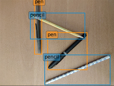
Conclusion
This post described how to create an efficient, end-to-end data-gathering pipeline in Amazon Ground Truth for an object detection model. Try out this process yourself next time you are creating an object detection model. You can modify the post-processing annotations to produce labeled data in the Pascal VOC format, which is required for models like Faster RCNN. You can also adopt the basic framework to other data-labeling pipelines with job-specific modifications. For example, you can rewrite the annotation post-processing procedures to adopt the framework for an instance segmentation task, in which an object is labeled at the pixel level instead of drawing a rectangle around the object. Amazon Ground Truth gets regularly updated with enhanced capabilities. Therefore, check the documentation for the most up to date features.
About the Author
 Arkajyoti Misra is a Data Scientist working in AWS Professional Services. He loves to dig into Machine Learning algorithms and enjoys reading about new frontiers in Deep Learning.


